Chemical equilibration of strangeness

Abstract

Thermal models are very useful in the understanding of particle production in general and especially in the case of strangeness. We summarize the assumptions which go into a thermal model calculation and which differ in the application of various groups. We compare the different results to each other. Using our own calculation we discuss the validity of the thermal model and the amount of strangeness equilibration at CERN-SPS energies. Finally the implications of the thermal analysis on the reaction dynamics are discussed.

Invited talk given at the Int. Symposium on Strangeness in Quark Matter 1997, Santorini (Greece), April 14 – 18, 1997

1 Introduction

Strange particles and other heavy flavors play always a special role in the analysis of hadronic collisions since they carry a new quantum number not present in the incoming nucleons or nuclei. Therefore they are considered as one of the most promising tools for learning more about the dynamics of heavy ion collisions. Especially, their use as a signature for Quark-Gluon Plasma (QGP) formation was proposed long ago [1, 2]. The argument is based on the different time scale for equilibration of strangeness due to the reduced kinematic threshold in the QGP [3]. There is a clear enhancement of strange particle production in heavy ion collisions compared to nucleon-nucleon collisions [4, 5]. Especially, the multistrange baryon yields increase drastically from $p+p$ to $A$+$A$ [6].

This interpretation of the measured abundances in favor of a QGP formation has basically two strategies. First, dynamical arguments show that the lifetime of a QGP is enough to reproduce the (still not complete) strangeness equilibration [7, 8]. Second, the strange particle ratios are compatible with a sudden disintegrating QGP [9, 10]. However, the interpretation is still controversial [11] and alternative explanations without QGP formation are also successful [12, 13, 14].

The various microscopic production models for strange particles in heavy ion collisions go from perturbative calculations on parton level [8] to string-string interactions (color ropes) [12] to hadronic rescattering mechanisms [14]. We leave out the complicated question of the dynamics of strange quark production and address the simpler question of whether strangeness production already saturates in heavy ion collisions, i.e. it reaches chemical equilibrium in the final state. This investigation concentrates only on the final freeze-out and it implicitly assumes that the particle production may be described in a statistical or even thermal model. Therefore one has first to address the more general question whether the overall particle production is given by a thermal production mechanism. The answers will in general depend on the particle species, the center of mass energy and the volume.

The recent success in the statistical interpretation of particle production in elementary reactions like $e^{+}+e^{-}$ [15] and $p+p$ ($\bar{p}+p$) [16] as well as in heavy ion reactions at various energies [17, 18] triggered a revival of the thermal model applications. Therefore we will concentrate to review the status of the thermal model for particle production in general and in the special case of strangeness. In section 2 we will present a hitch hikers guide through thermal models addressing various points which differ in the application of the model by various groups. Section 3 is devoted to the discussion of our own calculation done for CERN-SPS energies. In section 4 we discuss the implications from the thermal analysis of particle production and give a general conclusion.

2 The thermal model

A lot of publications have addressed the question of particle production within the thermal model. This can be seen in table 1 where only recent ones have been included. The list is certainly not complete due to ignorance or due to series of publications of one group where we took only the most recent one. Even if the thermal formalism is used for the same collision system the results vary (see table 1) because the model is applied in various approximations and extensions which we would like to discuss first. This will help to understand the differences in the calculations and the conclusions about the physics of these reactions.

Table 1: Summary of calculations addressing the chemical freeze-out in various collisions.

• 	$\sqrt{s}$
  collision	(MeV)	$T$ (MeV)	$\mu_{B}$ (MeV)	$\gamma_{s}$	ref.
  $e^{+}$ + $e^{-}$	29.0	$196\pm 7$	-	1	[19]
  $e^{+}$ + $e^{-}$	91.5	$261\pm 9$	-	1	[20]
  $e^{+}$ + $e^{-}$	29.0	$163.6\pm 3.6$	-	$0.724\pm 0.045$	[21]
  $e^{+}$ + $e^{-}$	91.5	$160.6\pm 1.7$	-	$0.675\pm 0.020$	[21]
  p+p	19.5	$161\pm 31$	$200\pm 37$	$0.22\hbox{\phantom{\rm 0}}\pm 0.05$	[22]
  p+p	19.5	$190.8\pm 27.4$	-	$0.463\pm 0.037$	[16]
  p+p	27.5	$169.0\pm 2.1$	-	$0.510\pm 0.011$	[16]
  Si+Au	05.3	$100.2$	$559.5$	1	[23]
  Si+Au	05.3	$127\pm 8$	$485\pm 70$	$0.5\pm 0.2^{\rm a}$	[24]
  Si+Au	05.3	$140\pm 5$	$555\pm 33$	$1$	[26]
  Si+Au(Pb)	05.3	$130\pm 10$	$540$	$1$	[17]
  Si+Au	05.3	$110\pm 5$	$540\pm 20$	$1$	[27]
  Au+Au	04.7	$100\pm 4$	-	$1$	[28]
  S+S	19.5	$170$	$257$	$1$	[29]
  S+S	19.5	$197\pm 29$	$267\pm 21$	$1.00\hbox{\phantom{\rm 0}}\pm 0.21$	[22]
  S+S	19.5	$185$	$301$	$1$	[30]
  S+S	19.5	$192\pm 15$	$222\pm 10$	$1$	[26]
  S+S	19.5	$182\pm 9$	$226\pm 13$	$0.73\hbox{\phantom{\rm 0}}\pm 0.04$	[31]
  S+S	19.5	$202\pm 13$	$259\pm 15$	$0.84\hbox{\phantom{\rm 0}}\pm 0.07$	[32]
  S+Ag	19.5	$191\pm 17$	$279\pm 33$	$1$	[26]
  S+Ag	19.5	$180.0\pm 3.2$	$238\pm 12$	$0.83\hbox{\phantom{\rm 0}}\pm 0.07$	[31]
  S+Ag	19.5	$185\pm 8$	$244\pm 14$	$0.82\hbox{\phantom{\rm 0}}\pm 0.07$	[32]
  S+Pb	19.5	$172\pm 16$	$292\pm 42$	$1$	[33]
  S+W	19.5	$190\pm 10$	$240\pm 40$	$0.7$	[34]
  S+W	19.5	$190$	$223\pm 19$	$0.68\hbox{\phantom{\rm 0}}\pm 0.06$	[10]
  S+W	19.5	$196\pm 9$	$231\pm 18$	$1$	[26]
  S+Au(W,Pb)	19.5	$165\pm 5$	$175\pm 5$	$1$	[18]
  S+Au(W,Pb)	19.5	$160$	$171$	$1$	[35]
  S+Au(W,Pb)	19.5	$160.2\pm 3.5$	$158\pm 4$	$0.66\pm 0.04$	[32]

  
  

• ^a only guessed.

2.1 Basic particle yields

In the thermal model the particle yields are given by a temperature $T$ and a volume $V$ common for all particles. If one considers only particle ratios then in most of the applications the ratio is independent of $V$ as it was shown in [36]. In addition the abundance of a particle depends on its conserved quantum numbers. This is either regulated by chemical potentials in the grand canonical description or by restricting the partition function only to states which have the same quantum number as the fireball, i.e. canonical treatment. The basic expression for the abundance $N_{j}$ of a particle of species $j$ is given by

$$N_{j}=\lambda_{j}\frac{\partial\ln Z(T,V,...)}{\partial\lambda_{j}}.$$ (1)

All models fulfill this basic requirement with the exception of the work of Hoang for $e^{+}$ + $e^{-}$ collisions [19, 20]. Some empirical formula for the particle yields is used, which is badly justified. Therefore all results in [19, 20] should be taken with care.

2.2 Statistic

It is obvious that one should use quantum statistics for calculating the partition function, i.e. to use Bose and Fermi statistics. However, for practical reasons one usually switches to the Boltzmann approximation. The error for pions is at $T=150$ MeV ($T=200$ MeV) 9.4% (11.3%), respectively and for kaons at the same temperature 0.5% (1.1%), respectively. This estimate suggest to use Bose statistic for pions while for all other heavier particles the Boltzmann approximation is valid. Note, that for entropy and pressure the differences between Boltzmann statistic and Bose/Fermi statistic are larger. Going to very low temperatures and/or high densities the use of the right statistic is unavoidable [37].

2.3 Canonical vs grand canonical

The strong interaction conserves exactly the quantum numbers charge $Q$, baryon number $B$ and strangeness S. This has to be taken care in a statistical approach and therefore the question arises which statistical ensemble concerning these quantum numbers one has to use [38, 39, 28]. As a first estimate one usually considers the fluctuations $\Delta O$ of a conserved quantity $O$ in the grand canonical treatment [40]

$$\Delta O=\sqrt{\langle O^{2}\rangle-\langle O\rangle^{2}}\propto\sqrt{N},$$ (2)

where $N$ is the number of all particles carrying a non zero quantum number $O$. In order to be better than 10% this suggest to use canonical treatment when the number of corresponding particles is below 100. However, in practice – depending on the observable calculated – already a much smaller total amount $N$ of particles is enough to have accuracy better then 10% using the grand canonical ansatz. This was shown in [38] and also recently in [28], where particle ratios already seem to saturate for number of participating baryons of around 30–40.

In the applications for heavy ion collisions the grand canonical treatment is justified when single particle yields are addressed [41]. We tested the difference in the resulting thermal parameters using canonical and grand canonical treatment for strangeness. We saw only minor differences between both calculations for ultra-relativistic heavy ion collisions. However, for strange particle correlations the use of the canonical ansatz is recommended [41].

If the thermal model is applied to inelastic two body collisions at high energies the analysis should be done using the canonical ensemble. Among the calculations in table 1 this was only performed by Becattini [21, 16]. All other calculations concerning $p$ + $p$ and $e^{+}$ + $e^{-}$ have to be taken with care. For example, we made a least mean square fit ($\chi^{2}$-fit) using the grand canonical ensemble for charge, baryon number and strangeness for particle production in p+p collisions at $\sqrt{s}=27.5$ GeV. The experimental input data are the same as in the work of Becattini et al [16] and the resonances included are very much the same. The fit to the data gets worse but the fit temperature stays very much the same and turned out to be $T=160$ MeV but the strangeness suppression $\gamma_{s}$ (see Section 2.8) is reduced to $\gamma_{s}=0.35$ compared to $\gamma_{s}=0.51$ in [16]. The canonical treatment suppresses the strangeness production due to associate pair production leading naturally to lower strangeness yields as compared to elementary reactions.

The chemical potentials in the grand canonical approach are first of all Lagrangian multipliers for the conserved charge. However, the strange quark chemical potential $\mu_{\rm s}$ plays a special role in the interpretation of strange particle abundances [42]. It is zero in a strangeness neutral QGP but has usually non-zero values in an equilibrated hadron gas. The $\mu_{\rm s}=0$ line in the $T$-$\mu_{\rm B}$ plane calculated for an equilibrated hadron gas is close to the expected QGP phase transition line [25, 26]. This similarity leads to speculations about the meaning of the $\mu_{\rm s}=0$ line which were extensively discussed in [25, 26].

2.4 Isospin

Isospin breaking effects become important when target and projectile nuclei are large. In most of the thermal models isospin is neglected. We may estimate the effect of isospin breaking to be of order $1-2Z/A$. This leads in S+Au collisions to a correction of order 10 % and for Pb+Pb of order 20%. Therefore one should take charge and baryon number separately into account especially for isospin sensitive quantities like $\pi^{+}/\pi^{-}$ or $K^{+}/K^{-}$. All above listed models in table 1 neglect isospin in the case of a heavy target. As an example one may discuss the $\pi^{+}/\pi^{-}$ ratio which is different from one in the low $p_{T}$-region of Au + Au [43] and Pb + Pb [44] collisions by chemical equilibration arguments. This ratio is sensitive to isospin violating weak decays as discussed in [45]. But in addition the isospin asymmetry in the colliding nuclei plays an important role and this was neglected in [45].

The isospin SU(2) may be treated exactly like in [39] or to a very good approximation as an U(1) $\times$ U(1). Then one usually conserves baryon number and charge or on valence quark level the net number of u-quarks and net number of d-quarks. In a grand canonical treatment it is equivalent to introduce chemical potential for baryon number and charge or for up and down quarks.

2.5 Finite volume correction

Calculating the partition function one switches from the summation over the states to the integral representation

$$\sum\limits_{k}^{\rm states}\longrightarrow\int{\mathrm{d}}^{3}\vec{k}\mskip 5.0mu plus 5.0mug(\vec{k})=4\pi\int{\mathrm{d}}k\mskip 5.0mu plus 5.0muk^{2}g(k),$$ (3)

where $g(k)$ is the density of state. If the volume is small $g(k)$ is very different from the infinite volume limit $V/(2\pi)^{3}$ and often approximated by [46, 40]

$$g(k)=\frac{V}{(2\pi)^{3}}-\frac{S}{32\pi^{2}k}+\frac{L}{32\pi^{2}k^{2}},$$ (4)

where $V$ is the volume $S$ the surface and $L$ the circumference of the box. This is only an approximate formula derived for Dirichlet boundary conditions and the error is of the order of the last term. This kind of correction was applied in [17, 18, 23, 29].

Going to $p$ + $p$ collisions one might think that this kind of correction might be very important. However, we like to argue that in this case and also for ultra-relativistic heavy ion collisions it is reasonable to use the continuous density of state for the following reason. In equation (4) it is assumed that the states have to fulfill Dirichlet boundary conditions on the edge of the interaction volume. This is only true for an infinite high potential well. In reality there is no such large binding force for the particles squeezing its wave function to the reaction volume. The particle energies are much higher than a nuclear binding potential. Therefore we think that the use of the continuous density of state is appropriate as long as the thermal energies are above a mean field potential which serves as a confining box.

2.6 Resonances

It is now commonly agreed that the particle production is dominated by resonance production mechanisms. Therefore the resonance states are included in the partition function of all calculations in table 1 except for [19, 20]. On the other hand their decay is sometimes neglected [26, 30] when calculations are compared to experimental data. Some of the publications restrict their discussion to strange baryon ratios. Then the resonance contribution may be restricted to the inclusion of the $\Sigma^{0}$ decay which feeds into the $\Lambda$ yield. This gives a reasonable estimate for the fugacities. If, however, kaons are included in the chemical analysis one has to consider the sizeable feeding from resonances and its omission is hardly comprehensible. In the treatment of resonances the following items are important.

2.6.1 Number of resonance states

The modeling of a steady state hadron gas needs the input of all resonance states leading to the bootstrap description of thermodynamics of strong interacting matter [47]. As a result one gets an exponential increasing density of resonance states

$$\rho(m)\propto m^{a}\exp(m/T_{\rm H})$$ (5)

with the consequence of a limiting temperature $T_{\rm H}$, called Hagedorn temperature. In the applications for hadronic collisions it is assumed that only a finite range in the resonance mass spectrum is equilibrated. The finite volume of the fireball leads to a finite total energy giving an upper limit in the mass spectrum to be considered. This estimate corresponds practically to an infinite mass spectrum. It arises the question whether already a much lower cut in the resonance spectrum can be justified. If chemical equilibrium is build up via secondary interactions than the limited life time of the fireball leads to a limited amount of equilibrated resonance states. If, however, the hadronization in elementary p + p collisions follows the chemical equilibrium abundances – and this seemed to be the case [16] – then it is hard to argue for the omission of the higher mass states, especially if the temperature is around 200 MeV. Nevertheless the known resonance states fade at masses around 2 GeV and therefore the calculations have to be restricted to a finite number of states.

The applied cut in the resonance states of the various groups is arbitrary and given by practical considerations. It has been shown that there is a small influence on the extracted thermal parameters on the cut in the resonance spectrum [22, 15, 16]. The temperature fitted to measured particle ratios shows a maximum at a resonance cut-off at $\approx 1.5$ GeV. It is interesting to note that fits to the experimental known density of states $\rho(m)$ by the bootstrap formula in equation (5) start to deviate at the same mass of 1.5 GeV [48]. Therefore one should be aware that thermal fits at temperatures higher than $\approx 170$ MeV are biased from the resonance spectrum which is taken into account.

2.6.2 Branching of resonances

Not only the poor knowledge of resonance states around 2 GeV has some influence on the analysis for high temperatures, but also the branching ratios. Already at 1.5 GeV they are starting of getting basically unknown and the various groups use some “educated guess” [27].

2.6.3 Resonance width

Usually the width of a resonance is neglected. This means that in the Boltzmann factor $\exp(-\sqrt{m^{2}+p^{2}}/T)$ the mean mass $\bar{m}$ of a resonances is taken. This assumption was made in nearly all calculations of table 1. For broad resonances this is a bad approximation. One suggestion to improve this is to distribute the mass states of a resonance according to a Breit-Wigner form [15, 16, 31, 32]. This means that the mass shell constraint in the Lorentz invariant momentum integration for the partition function is replaced by [49]

$$\int{\mathrm{d}}^{4}p\mskip 5.0mu plus 5.0mu\delta\left(p_{\mu}p^{\mu}-m_{0}^{2}\right)\theta\left(\sqrt{p_{\mu}p^{\mu}}\right)$$

$$\longrightarrow\int{\mathrm{d}}^{4}p\mskip 5.0mu plus 5.0mu\frac{m_{0}\Gamma}{\left(p_{\mu}p^{\mu}-m_{0}^{2}\right)^{2}-m_{0}^{2}\Gamma^{2}}\mskip 5.0mu plus 5.0mu\theta\left(\sqrt{p_{\mu}p^{\mu}}-m_{\rm thres}\right),$$ (6)

where $\Gamma$ is the width of the resonance and $m_{\rm thres}$ a threshold for the resonance production. The inclusion of the width is important for the yield of the $\rho$-meson. It turned out to improve the fits in p + p collisions [16].

2.7 Repulsive interaction

The experimental particle yields and ratios are determined at (chemical) freeze-out. One usually assumes that the system is already such diluted that the interactions have effectively cease to exist. Then the problem of residual interactions don’t occur. However, in the analysis of SPS energies the chemical freeze-out temperature seems to be around 160–200 MeV (see table 1). At this temperature the particle density is still very high and one has to ask how density corrections influence the particle yields. In the bootstrap model of Hagedorn the dominant part of the attractive strong interaction is effectively taken into account by including the higher resonance states [47]. However, at high densities the repulsive part have to be accounted for, too. It is popular to use an excluded volume correction [50, 51, 52, 53] where the hadrons are treated as finite size hard core particles. In the early suggestions [50, 51] the real physical particle density $n^{\rm phy}$ is related to the ideal or point particle density $n^{\rm point}$ by

$$n^{\rm phy}=\alpha^{-1}n^{\rm point},$$ (7)

where $\alpha$ is either given by the total point particle energy density $\varepsilon_{0}$ and the bag constant $B$, i.e. $\alpha=1+\varepsilon_{0}/(4B)$ [50], or by $\alpha=1+\sum_{j}V^{0}_{j}n_{j}^{0}$ where $V^{0}_{j}$ is a hard core volume and $n_{j}^{0}$ the point particle density of species $j$ [51]. The important point is that such a treatment don’t influence particle ratios since the factor is common for all particle species and therefore don’t change the thermal analysis. The volume $V$ which appears as a common factor has to be regarded as the point particle volume and the physical volume is then given by $\alpha V$.

The above described correction is thermodynamically not consistent [50, 51] and improvements have been suggested [52, 53, 54] (for an extended discussion see [55]). One may divide them basically into mean field approaches like [54] or thermodynamically consistent excluded volume corrections like [52, 53] or both [52]. These models contain additional parameters which characterize either the hard core size $V^{0}_{j}$ or the mean field coupling $K_{j}$ of a particle $j$. If $V^{0}_{j}$ or $K_{j}$ are different for various $j$ then they influence the particle ratios. The only publications in table 1 which have such an influence on particle ratios due to repulsions are [23, 29, 30]. In [23, 29] the effect is minimal since the mean field coupling $K_{B}=680$ MeV fm³ of baryons and anti-baryons is similar to the one of mesons $K_{M}=600$ MeV fm³. The studies in [30] show the repulsion effect for the heavy baryons. The extracted $\mu_{B}$ in [30] differs from the other results of table 1. Tiwari et al take for the hard core size of a particle the MIT bag model result of $V^{0}_{j}=m_{j}/(4B)$, i.e. the hard core volume scales with its mass. Therefore the massive baryons are additionally suppressed by their size. This has to be compensated by a higher $\mu_{B}$.

2.8 Off-equilibrium phenomenology

Since the life time of a fireball created in heavy ion collisions is very short and the dynamics is very rapid it cannot be expected that the production of particles of all kind follow the equilibrium statistics. In order to study the deviations from equilibrium quantitatively one introduces over-saturation/suppression factors $\gamma$ which measure the deviations from full equilibrium. For strangeness they were first introduced by Rafelski [42] in a phenomenological way. They were defined by

$$\gamma=\frac{\rm actual\mskip 5.0mu plus 5.0mudensity}{\rm equilibrium\mskip 5.0mu plus 5.0mudensity}.$$ (8)

It has been shown [56] that the thermodynamically correct way of defining such a parameter is to define them as fugacity

$$\gamma=\exp(\mu/T),$$ (9)

as it is done in a grand canonical approach. This is in accordance with the model of relative chemical equilibrium. This means that only a subset of particles is in chemical equilibrium among each other and the deviation to another set of particles is parametrized by $\gamma$. Examples for such applications are the strangeness suppression $\gamma_{s}$ [42], the pion chemical potential [57] or general meson and baryon suppression factors [58].

With the help of suppression factors one is able to study the approach to chemical equilibrium. Some of the calculations in table 1 allow for such a suppression and some don’t. Since we know from $p$ + $p$ collisions [16] that strangeness is suppressed by roughly a factor of 2 one should always allow the suppression possibility in heavy ion reactions. In table 1 all calculation which don’t allow strangeness suppression have 1 in the column for $\gamma_{s}$.

2.9 Restricted acceptance

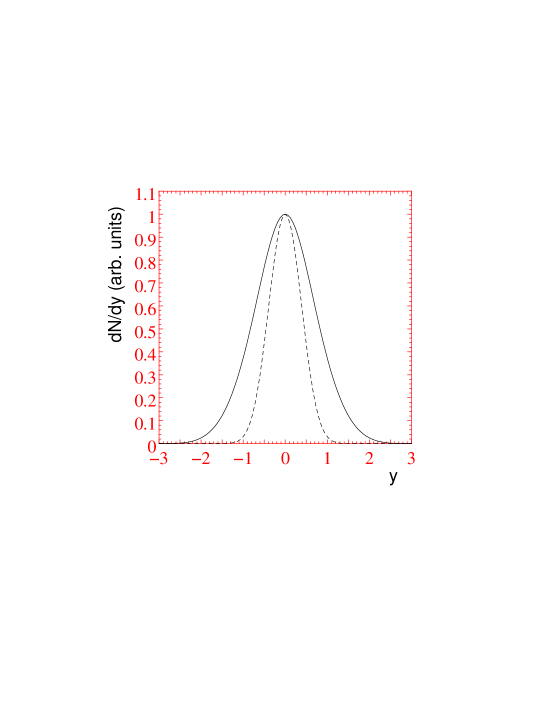
Figure 1: Pion (solid line) and proton (dashed line) rapidity distribution of a static fireball at a temperature of $T=150$ MeV normalized to one at central rapidity.

If thermal equilibrium is established it is either globally or locally. In most of the cases as for example in S+S collisions at CERN-SPS the rapidity distributions of baryons and pions are very different in shape [59]. This suggest that the freeze-out parameters vary locally. One way to demonstrate this was assuming a rapidity dependence of the baryon chemical potential as done in [56]. However, the proper treatment of locally varying thermal parameters is via hydrodynamics [60]. On the other hand, if the differences are small, the use of one global fireball in the analysis of $4\pi$ data is appropriate and the result should be understood as a global average.

The most reliable way to analyze particle yields and ratios is using $4\pi$ integrated data. This avoids problems due to kinematic cuts. Addressing particle ratios in restricted kinematic regions needs a model for the particle spectra, too. Particle spectra are much more sensitive to the dynamics and one needs more assumptions and knowledge about the space-time evolution in longitudinal and transverse direction. Therefore we recommend the use of $4\pi$ data for the study of chemical equilibration.

Most of the analysis in table 1 is applied to particle ratios in a restricted kinematic region. The reason is that most of the particle ratios are only measured in a kinematic window. This requires that the calculation is cut to the experimental acceptance and the knowledge of the particle spectra is unavoidable.

We like to demonstrate how much results in principle may depend on assumptions about the longitudinal dynamics at freeze-out. The two extreme scenarios are a static fireball and the Bjorken boost-invariant scenario [61]. In a static fireball the rapidity distribution using Boltzmann approximation is given by

$$\frac{{\mathrm{d}}N^{\rm static}}{{\mathrm{d}}y}(y) = \frac{Vgm^{2}T}{2\pi^{2}}\exp\left[-(m\cosh(y)-\mu)/T\right]$$ (10)

$$\times\left[\frac{1}{2}+\frac{T}{m\cosh(y)}+\left(\frac{T}{m\cosh(y)}\right)^{2}\right],$$

while in the Bjorken case it is

$$\frac{{\mathrm{d}}N^{\rm Bjo}}{{\mathrm{d}}y}(y)\propto\frac{gm^{2}T}{2\pi^{2}}\mskip 5.0mu plus 5.0mu\exp(\mu/T)\mskip 5.0mu plus 5.0mu{\rm K}_{2}(m/T).$$ (11)

It is $V$ the volume $g$ the spin degeneracy and $m$ the mass. As an example we show in figure 1 the pion and proton rapidity distributions for a static fireball given by equation (10). The pion and proton distribution are normalized to one and therefore its ratio at midrapidity is one. In the Bjorken scenario the ratio of pions to protons is given by the integration over rapidity in equation (10) resulting in the expression of equation (11). In our example it would be $(dN^{p}/dy)/(dN^{\pi}/dy)=0.54$. Since the mass of pions and protons are very different the effect is most pronounced in the example. We show in Section 3 that in practice the differences between both scenarios are minor using the example of S+Au collisions.

The experimental rapidity distributions are broader than given by a static source (10) but not infinite broad like in the case of Bjorken scaling. Since the experimental width of various rapidity spectra is very similar a thermal analysis in a restricted rapidity range usually assumes Bjorken scaling and uses equation (11) for particle yields.

3 Results from thermal model analysis

The strength of the thermal model is that most of the particle ratios can be explained by only a few parameters. However, from table 1 one cannot see how well the thermal model works and where the deviations start. Therefore we show the results of one calculation in more detail. We perform a thermal model calculation which has the following characteristic [32]:

• All hadronic states up to 1.7 GeV in mass are included.

• Pions follow the Bose statistic while for all other hadrons the Boltzmann approximation is used.

• The resonances are populated including their width according to equation (2.6.3). The Breit-Wigner distribution in mass is restricted to a range of two times the width [15].

• When comparing to experimental results we include the feeding of resonances and in the case of S+Au we also include the $p_{T}$-cut of the experimental ratios.

• For S+S and S+Ag strangeness is treated in the canonical formalism while for S+Au we use the grand canonical ensemble. Baryon number is regulated via a chemical potential. Isospin symmetry is assumed.

• No finite size correction and no repulsive interaction is included.

We analyze experimental particle yields in two ways. On the one hand we perform a $\chi^{2}$-fit to $4\pi$ data of S+S and S+Ag collisions and to central particle ratios in S+Au collisions. The second possibility is to display the experimental particle ratios in the $T$-$\mu_{B}$ plane and look for overlap regions of the various bands.

Table 2: Result of a fit to experimental $4\pi$ data of S+S and S+Ag collisions at CERN-SPS. The data are all measured by the NA35 collaboration.

• 	S+S			S+Ag
  	calculation	data	ref.	calculation	data	ref.
  $h^{-}$	83.7	$94\pm 5$	[59]	151	$160\pm 8$	[62]
  $K^{+}$	12.7	$12.5\pm 0.4$	[63]	23.0
  $K^{-}$	7.13	$6.9\pm 0.4$	[63]	13.3
  $K_{s}^{0}$	9.70	$10.5\pm 1.7$	[64]	17.8	$15.5\pm 1.5$	[64]
  $\Lambda$	8.69	$9.4\pm 1.0$	[64]	14.4	$15.2\pm 1.2$	[64]
  $\bar{\Lambda}$	1.84	$2.2\pm 0.4$	[64]	2.54	$2.6\pm 0.3$	[64]
  $p-\bar{p}$	22.6	$20.2\pm 2.0$	[59]	38.1	$34\pm 4$	[62]
  $\bar{p}^{\rm a}$	1.93	$1.15\pm 0.4$	[65]	2.99	$2.0\pm 0.8$	[65]
  T (MeV)	$202\pm 13$			$185\pm 8$
  V (fm3)	$81.5\pm 39.4$			$275\pm 84$
  $\gamma_{s}$	$0.84\pm 0.07$			$0.82\pm 0.07$
  $\lambda_{q}$	$1.532\pm 0.038$			$1.552\pm 0.041$
  $\chi^{2}$/dof	11.6/4			6.72/2

  
  

• ^a The experimental value is extrapolated to $4\pi$ assuming the same rapidity shape as the $\bar{\Lambda}$.

In table 2 we show the result of a $\chi^{2}$-fit to $4\pi$ data from the NA35 collaboration (see references in table 2). In S+Ag collisions the assumed isospin symmetry is slightly violated. In order to estimate the size of the effect we have also done a fit using separate chemical potentials for up and down quarks and including the total net charge. In the case of S+Ag collisions the result is a slightly larger $\lambda_{d}=1.572\pm 0.053$ as compared to $\lambda_{u}=1.521\pm 0.034$. This is expected by the larger amount of incoming u-quarks.

The calculations are very similar to the one of Becattini [31] but note that in the case of S+S collisions a different input set of experimental data is used. Therefore we get a much higher temperature for S+S while for S+Ag both calculations basically agree. The differences between them are small deviations in the input resonances states, their branching and the treatment of the $\eta$-$\eta^{\prime}$ mixing.

Looking at the result in more detail one realizes that the thermal fit is not perfect, especially for S+S collisions ($\chi^{2}/{\rm dof}=11.6/4$). The largest deviations are in the anti-baryon yields. The high absorption cross section of this particles may explain the deviations.

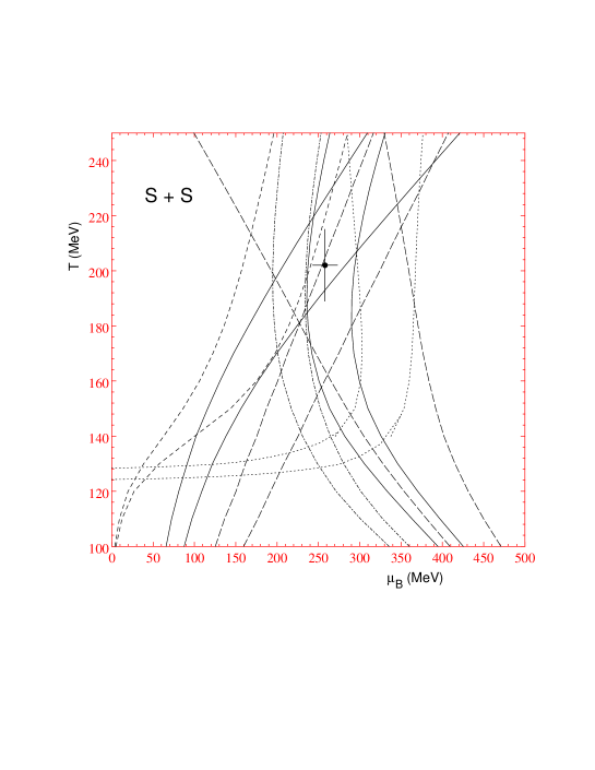
Figure 2: Experimental particle ratios in the $T$-$\mu_{B}$ plane for S+S collisions taking $\gamma_{s}=0.84$ and $V=81.5$ fm³. The bands along the abscissa correspond to the following ratios (going from left to right): $K^{-}/h^{-}$ (${\mathinner{\cdotp\cdotp\cdotp\cdotp\cdotp\cdotp}}$), $\Lambda/(p-\bar{p})$ (– – –), $\bar{\Lambda}/\Lambda$ (——), $\bar{p}/(p-\bar{p})$ (— — —), $h^{-}/(p-\bar{p})$ (— $\cdot$ —) $K^{+}/K^{-}$ (——) and $K_{s}^{0}/\Lambda$ (— — —). The point indicates the result of the $\chi^{2}$-fit in table 2.

A different way of displaying the quality of the thermal model approach is shown in figure 2 where in the $T$-$\mu_{B}$-plane various bands indicate experimental particle ratios. We changed to particle ratios because they are nearly independent of the volume. Since we use the canonical ensemble for strangeness we have a small influence of the particle ratios on the volume. We calculated the used experimental particle ratios from table 2. The errors of the ratios are determined by adding the individual errors quadratically. The bands correspond to the upper and lower bound on the experimental ratio. Note that a fixed volume was used.

In figure 2 we see no real overlap region of all particle ratios. Especially, the ratios containing the $h^{-}$ fail to cover the $\chi^{2}$-fit point which is given by the filled circle. We like to point out the possible sign of an enhanced entropy production seen in the $h^{-}$ as discussed in [10, 66]. Our present reevaluation of the experimental data confirms this possibility. We expect a stronger effect on an enhanced pion production in Pb+Pb collisions.

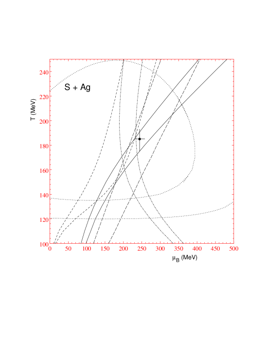
Figure 3: Experimental particle ratios in the $T$-$\mu_{B}$ plane for S+Ag collisions taking $\gamma_{s}=0.82$ and $V=275$ fm³. The bands along the abscissa correspond to the following ratios (going from left to right): $K_{s}^{0}/h^{-}$ (${\mathinner{\cdotp\cdotp\cdotp\cdotp\cdotp\cdotp}}$), $\Lambda/(p-\bar{p})$ (– – –), $\bar{\Lambda}/\Lambda$ (——), $\bar{p}/(p-\bar{p})$ (— — —) and $h^{-}/(p-\bar{p})$ (— $\cdot$ —). The point indicates the result of the $\chi^{2}$-fit in table 2.

In S+Ag collisions the quality of particle production using a thermal model is similar to the one in S+S as may be seen from the $\chi^{2}$ in table 2 or in figure 3 where we plotted again various ratios in the same way as in figure 2. All particle ratios, excluding $K_{s}^{0}/h^{-}$, have one common overlap at $T=170\pm 10$ MeV and $\mu_{B}=220\pm 10$ MeV. The inclusion of the $K_{s}^{0}/h^{-}$ ratio in the $\chi^{2}$-fit moves that result out of the otherwise common overlap. Excluding $K_{s}^{0}$ one gets for S+Ag collisions similar freeze-out parameters as for S+Au collisions below.

Table 3: Result of a fit to experimental central rapidity particle ratios in S+Au(W,Pb) collisions at CERN-SPS assuming Bjorken scaling. The extracted thermal parameters are $T=160.2\pm 3.5$ MeV, $\lambda_{q}=1.390\pm 0.012$ and $\gamma_{s}=0.656\pm 0.041$. It is $\chi^{2}/{\rm dof}=37.7/10$.

• S+Au	cal.	data	target	rapidity	$p_{T}$cut	ref.
  $D_{q}^{\rm a}$	0.0782	$0.088\pm 0.007$	Pb	2.3–3.0	0	EMU05[67]
  $p/\pi^{+}$	0.188	$0.19\pm 0.03$	Pb	2.6–2.8	0	NA44[68]
  $\bar{p}/\pi^{-}$	0.0262	$0.024\pm 0.009$	Pb	2.6–2.8	0	NA44[68]
  $\bar{p}/p$	0.139	$0.12\pm 0.02$	Pb	2.65–2.95	0	NA44[69]
  $\eta/\pi^{0}$	0.0816	$0.15\pm 0.02$	Au	2.1–2.9	0	WA80[70]
  $R_{K}^{\rm b}$	2.03	$2.14\pm 0.06$	W	2.5–3.0	1.0	WA85[6]
  $K^{+}/K^{-}$	1.57	$1.67\pm 0.15$	W	2.3–3.0	0.9	WA85[6]
  $K_{s}^{0}/\Lambda$	1.21	$1.4\pm 0.1$	W	2.5–3.0	1.0	WA85[71]
  $\bar{\Lambda}/\Lambda$	0.203	$0.196\pm 0.011$	W	2.3–3.0	1.2	WA85[72]
  $\Xi^{-}/\Lambda$	0.0967	$0.097\pm 0.006$	W	2.3–3.0	1.2	WA85[72]
  $\Xi^{+}/\Xi^{-}$	0.283	$0.47\pm 0.06$	W	2.3–3.0	1.2	WA85[72]
  $R_{\Omega}^{\rm c}$	0.145	$0.8\pm 0.4$	W	2.5–3.0	1.6	WA85[6]
  $\bar{\Omega}/\Omega$	0.430	$0.57\pm 0.41$	W	2.5–3.0	0	WA85[73]

  
  

• ^a $D_{q}=(h^{+}-h^{-})/(h^{+}+h^{-})$

• ^b $R_{K}=(K^{+}+K^{-})/K_{s}^{0}$

• ^c $R_{\Omega}=(\bar{\Omega}+\Omega)/(\Xi^{+}+\Xi^{-})$

There are not enough $4\pi$ data on S+Au collisions and therefore we switch to particle ratios. The analysis is inspired by the work of Braun-Munzinger et al [18]. However we take in our analysis only a subset of particle ratios from their list, excluding all ratios which don’t cover midrapidity $y_{\rm cm}=2.65$. For the particle yields we use the scaling assumption, i.e. equation (11) as it was done in [18]. In addition we change to the grand canonical ensemble for strangeness.

The result of the $\chi^{2}$-fit is given in table 3. We reproduce the temperature $T=160$ MeV as it was assumed in [18] but we got a slightly lower $\mu_{B}$ of 158 MeV. The main difference of our calculation to the one in [18] is that we allow strangeness suppression. The ratios sensitive to $\gamma_{s}$ are $\Xi^{-}/\Lambda$ and $R_{\Omega}=(\bar{\Omega}+\Omega)/(\Xi^{+}+\Xi^{-})$. The resulting low value of $\gamma_{s}=0.65$ is not in agreement with the assumption of full chemical equilibrium for strangeness as it was assumed in many calculations.

The result of table 3 shows that a thermal hadron gas model even with no complete strangeness equilibration is not able to reproduce all experimental data. Some serious deviations are not in the table like $\bar{\Xi}/\bar{\Lambda}=0.23\pm 0.02$ [72] which in the thermal model is given by $\bar{\Xi}/\bar{\Lambda}=0.135$. The disagreement in the multi-strange baryons might indicate the onset of non-equilibrium physics with the origin in a QGP formation [1]. This proposal was recently discussed in depth in [8].

We tested our result against the assumption of Bjorken scaling in rapidity and did the same fit assuming one static fireball, i.e. using equation (10) at $y=0$. We got a rather similar result of $T=158\pm 3$ MeV, $\lambda_{q}=1.408\pm 0.012$ and $\gamma_{s}=0.74\pm 0.05$. We see in the $\chi^{2}$-fit no large dependence on the assumption about the rapidity distribution.

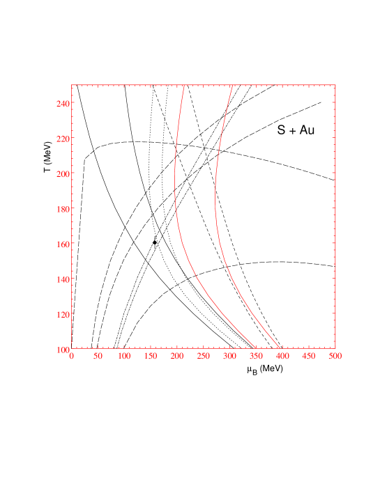
Figure 4: Experimental particle ratios in the $T$-$\mu_{B}$ plane for S+Au(W,Pb) collisions taking $\gamma_{s}=0.66$. In this plot the experimental kinematic cuts are not accounted for. The bands are explained along the upper part of the figure from left to right: $p/\pi^{+}$ (——), $K_{s}^{0}/\Lambda$ (– – –), $D_{q}$ (${\mathinner{\cdotp\cdotp\cdotp\cdotp\cdotp\cdotp}}$), $K^{+}/K^{-}$ (——), $\bar{\Lambda}/\Lambda$ (— $\cdot$ —), $\bar{\Xi}^{+}/\Xi^{-}$ (— — —) and the broad $\bar{\Omega}/\Omega$ (— — —). The point indicates the result of the $\chi^{2}$-fit in table 3.

We show in figure 4 some selected ratios from table 3 together with the point from the $\chi^{2}$-fit. Again we see no perfect agreement but a rather broad region where various bands concentrate.

The statistical error in the $\chi^{2}$-fit is determined by the region where $\chi^{2}$ increases by one unit from its minimum. However, from the figures 2, 3 and 4 one sees that the systematic error of the model applied is much larger. From the figures we conclude that the freeze-out temperature in heavy-ion collisions is still very uncertain and one has in fact to take a range of $T^{\rm chem}=150$–200 MeV.

The results on sulphur induced collisions at CERN-SPS indicate no full strangeness equilibration but one is very close to it. The slightly higher $\gamma_{s}$ in the smaller collision systems may be a result of having no multi-strange particles in the $\chi^{2}$-fit.

4 Conclusions from thermal models

Since the application of a statistical model to multi-particle production by Fermi [74] its validity is under debate. Therefore we would first like to make some general remarks. Thermodynamics is first of all a formalism which may be derived from statistical (quantum) mechanics in the infinite volume limit. The basic assumption going in is that all states which are allowed by conservation laws, including energy conservation, are equal probable. We get the microcanonical formalism. Going to the canonical formalism only states sharing the same total energy have the same probability which is proportional to $\propto\exp(-E/T)$. The equal probability is usually violated in elementary reactions where the final state probability is given by the corresponding matrix element. Therefore the general opinion is that in elementary reaction the thermal model has no justification.

However, a large number of particles in the final state suggests to use a statistical approach. Therefore the thermal model was applied for elementary reactions and one gets reasonable agreement [15, 16]. This observation suggest that if only enough energy is available the particle production is dominated by the statistical component and dynamical aspects are of minor importance. In addition Becattini [15, 16] got the important result that there is an universal hadronization temperature in different elementary collision systems and it is independent on $\sqrt{s}$. The interpretation is that in the rest frame of the leading particle/parton the probability of producing a particle with energy $E$ is proportional to $\propto\exp(-E/T_{h})$. The hadronization temperature $T_{h}$ may be identified with the Hagedorn temperature $T_{H}$. In the interpretation of Hagedorn [47] it is not possible to create a system of higher temperature than $T_{H}$ unless there is a phase transition. The limiting temperature is seen in elementary reactions even at very high energies like in $p$+$\bar{p}$ at CERN [16]. The above described observation was also dubbed as statistical filling of phase space. We want to point out that there is a difference in the basic hadron production probability compared to the string models for hadronic reactions [31]. There the production probability goes basically like $\propto\exp(-m^{2}*k)$ [75] with $k$ being a universal constant.

The mechanism for chemical equilibration in nucleus-nucleus collisions is expected to be different from the one in elementary reactions. In nuclear reactions we assume that chemical equilibration is established by secondary interactions among the produced hadrons. Therefore we distinguish two mechanisms which bring the system to maximum entropy or chemical equilibrium.

• The production of particles, i.e. the hadronization or fragmentation, follows a statistical law and already at their production they are distributed according to maximum entropy. The ensemble average is done by averaging over many events in the experimental analysis.

• The maximum of entropy is build up in the classical sense by interactions among the particles until detailed balance is reached. The ensemble average is reached in each collision by the average over the lifetime of the system (engodic theorem).

The thermodynamical formalism cannot distinguish between both scenarios and one has to use dynamical arguments to justify one or the other mechanism.

Since at SPS-energies the chemical freeze-out temperatures and the chemical potentials are very similar in p+p collisions and in S+$A$ collisions (see table 1) one cannot use them to justify secondary interactions for chemical equilibrium. A superposition of p+p collisions explains most of the features in the nuclear collisions [76] with the exception of strangeness. Therefore we emphasize the importance of the measurement of strangeness because there the difference in p+p to $A$+$A$ is most clearly seen.

The freeze-out temperature is expected to decrease with increasing $A$, because freeze-out occurs when the mean free path is of the order of the size of the system. Such an effect is not observed in an unambiguous way, yet. So far only indications are seen as for example the decrease of chemical freeze-out in our analysis from S+S to S+Ag to S+Au. A clear sign for chemical equilibration due to secondary interactions would be a difference in the chemical freeze-out of p+p compared to a real heavy nucleus like Pb+Pb or Au+Au. Such an analysis hasn’t been performed yet but with the now analyzed data of Pb+Pb at CERN-SPS (see for example the various contributions to this proceedings) it will be possible soon. At the AGS we expect different freeze-out temperatures for Si+Au and Au+Au. The first results on Au+Au [28] go in this direction but we have to wait for the completion of the experimental data analysis.

Coming finally back to strangeness we have here a clear signal of the difference between elementary reactions and nuclear collisions. The strangeness suppression factor $\gamma_{s}$ is the quantitative measure for the strangeness enhancement in the thermal model. In p+p it is $\gamma_{s}\approx 0.5$ [16] but in nuclear collisions at CERN-SPS it is around 0.7-1 (see table 1). A strangeness enhancement is seen at the AGS, too [77], but the situation is not so clear in terms of the thermal ansatz. A consistent study of the $\gamma_{s}$ dependence has not been made. First there is no thermal analysis of the p+p interaction at the corresponding $\sqrt{s}$ and second the analysis at AGS assumes mostly full strangeness equilibration as it is seen in table 1. However, we have already remarked [11] that a $\gamma_{s}\approx 0.7$ is better for describing the data at AGS.

We have shown that the thermal model fits are not perfect including all measured particle species. The deviations are a source of debate. The various interpretations are that the thermal description is not valid at all, the hadronization of a QGP leaves non-equilibrium tracks in special hadron ratios [8], anti-baryons exhibit a large absorption [78] or the deviations are not serious [18]. The final answer will be given in the expected high statistic data of Pb+Pb in the future.

We summarize that there are strong signs of chemical equilibration in heavy ion collisions. Since there is already an equally good chemical equilibrium (excluding strangeness) in the basic p+p collisions chemical equilibrium cannot be used for justifying secondary hadronic collisions. (There are better signals for abundant secondary interactions like the collective flow studies [79].) However, the strangeness production is very different between both collision systems and it may be used as the chemometer for chemical equilibrium.

References

Additional Figure

Figure 5: Overview of table 1 in the $T$-$\mu_{B}$-plane. The plot uses color coding and information is lost using black and white. The plot is not included in the version appearing in Journal of Physics G

References

- [1] Rafelski J 1981 Workshop on future relativistic heavy ion experiments ed R Bock and R Stock (Darmstadt: GSI-report 81-6) p 282
- [2] Rafelski J and Müller B 1982 Phys. Rev. Lett. 82 1066
- [3] Koch P, Müller B and Rafelski J 1986 Phys. Rep. 142 167
- [4] Kinson J B et al 1995 Nucl. Phys. A 590 317c
- [5] Gaździcki M et al 1995 Nucl. Phys. A 590 197c
- [6] diBari N et al 1995 Nucl. Phys. A 590 307c
- [7] Letessier J, Rafelski J and Tounsi A 1994 Phys. Lett. 333B 484; Letessier J, Rafelski J and Tounsi A 1997 Phys. Lett. 390B 363
- [8] Rafelski J, Letessier J and Tounsi A 1996 Acta Phys. Pol. B 27 1035
- [9] Letessier J, Rafelski J and Tounsi A 1994 Phys. Lett. 323B 393
- [10] Letessier J, Tounsi A, Heinz U, Sollfrank J and Rafelski J 1995 Phys. Rev. D 51 3408
- [11] Sollfrank J and Heinz U 1995 Quark-gluon plasma vol 2 ed R C Hwa (Singapore: World Scientific) p 555
- [12] Sorge H 1994 Nucl. Phys. A 566 633c
- [13] Topor Pop V, Gyulassy M, Wang X N, Andrighetto A, Morando M, Pellegrini F, Ricci R A and Segato G 1995 Phys. Rev. C 52 1618
- [14] Capella A 1996 Phys. Lett. 387B 400
- [15] Becattini F 1996 Z. Phys. C 69 485
- [16] Becattini F and Heinz U 1997 hep-ph/9702274
- [17] Braun-Munzinger P, Stachel J, Wessels J P and Xu N 1995 Phys. Lett. 344B 43
- [18] Braun-Munzinger P, Stachel J, Wessels J P and Xu N 1996 Phys. Lett. 365B 1
- [19] Hoang T F and Cork B 1988 Z. Phys. C 38 603
- [20] Hoang T F 1994 Z. Phys. C 62 343
- [21] Becattini F 1996 Proc. of the XXXIII Eloisatron workshop on universality features in multihadron production and the leading effect (Erice) to be published (hep-ph/9701275)
- [22] Sollfrank J, Gaździcki M, Heinz U and Rafelski J 1994 Z. Phys. C 61 659
- [23] Davidson N J, Miller H G and von Oertzen D W 1991 Phys. Lett. 256B 554
- [24] Letessier J, Rafelski J and Tounsi A 1994 Phys. Lett. 328B 499
- [25] Asprouli M N and Panagiotou A D 1995 Phys. Rev. C 51 1445
- [26] Panagiotou A D, Mavromanolakis G and Tzoulis J 1996 Phys. Rev. C 53 1353
- [27] Cleymans J, Elliott D, Satz H and Thews R L 1997 Z. Phys. C 74 319
- [28] Cleymans J and Muronga A 1997 Phys. Lett. 388B 5; Cleymans J, Marais M and Suhonen E 1997 preprint nucl-th/9705014
- [29] Davidson N J, Miller H G, Quick R M and Cleymans J 1991 Phys. Lett. 255B 105; Davidson N J, Miller H G, von Oertzen D W and Redlich K 1992 Z. Phys. C 56 319
- [30] Tiwari V K, Singh S K, Uddin S and Singh C P 1996 Phys. Rev. C 53 2388
- [31] Becattini F 1997 this proceedings
- [32] Sollfrank J et al 1997 in preparation
- [33] Andersen E et al 1994 Phys. Lett. 327B 433
- [34] Redlich K, Cleymans J, Satz H and Suhonen E 1994 Nucl. Phys. A 566 391c
- [35] Spieles C, Stöcker H and Greiner C 1997 nucl-th/9704008
- [36] Cleymans J 1997 Proc. of Third Int. Conf. on Physics and Astrophysics of Quark-gluon plasma (Jaipur) to appear, nucl-th 9704046
- [37] Lee K S and Heinz U 1993 Phys. Rev. D 47 2068
- [38] Rafelski J and Danos M 1980 Phys. Lett. 97B 279; Hagedorn R and Redlich K 1985 Z. Phys. C 27 541; Cleymans J, Suhonen E and Weber G M 1992 Z. Phys. C 53 485
- [39] Redlich K and Turko L 1980 Z. Phys. C 5 201
- [40] Pathria R K 1972 Statistical Mechanics (Oxford: Pergamon Press) p 487
- [41] Cleymans J and Koch P 1991 Z. Phys. C 52 137
- [42] Rafelski J 1991 Phys. Lett. 262B 333
- [43] Ahle L et al 1995 Nucl. Phys. A 590 249c
- [44] Bøggild H et al 1996 Phys. Lett. 372B 343
- [45] Arbex N, Ornik U, Plümer M, Schlei B R and Weiner R M 1997 Phys. Lett. 391B 465
- [46] Hill D L and Wheeler J A 1953 Phys. Rev. 89 1102
- [47] Hagedorn R 1971 CERN-report 71-12; Hagedorn R 1995 Hot Hadronic Matter: Theory and Experiment, ed J Letessier et al (New York: Plenum) p 13
- [48] Tounsi A, Letessier J and Rafelski J 1994 Hot Hadronic Matter: Theory and Experiment, ed J Letessier et al (New York: Plenum) p 105
- [49] Sollfrank J, Koch P and Heinz U 1991 Z. Phys. C 52 593
- [50] Hagedorn R and Rafelski J 1980 Phys. Lett. 97B 136
- [51] Cleymans J, Redlich K, Satz H and Suhonen E 1986 Z. Phys. C 33 151; Heinz U, Subramanian P R, Stöcker H and Greiner W 1986 J. Phys. G: Nucl. Phys. 12 1237
- [52] Rischke D H, Gorenstein M I, Stöcker H and Greiner W, 1991 Z. Phys. C 51 485
- [53] Uddin S and Singh C P 1994 Z. Phys. C 63 147
- [54] Kapusta J I and Olive K A 1983 Nucl. Phys. A 408 478
- [55] Venugopalan R and Prakash M 1992 Nucl. Phys. A 546 718
- [56] Slotta C, Sollfrank J and Heinz U 1995 Proc. of Strangeness in Hadronic Matter (Tucson) ed J Rafelski (Woodbury: AIP Press) p 462
- [57] Kataja M and Ruuskanen P V 1990 Phys. Lett. 243B 181
- [58] Letessier J, Rafelski J and Tounsi A 1994 Phys. Lett. 321B 394
- [59] Bächler J et al 1994 Phys. Rev. Lett. 72 1419
- [60] Sollfrank J, Huovinen P, Kataja M, Ruuskanen P V, Prakash M and Venugopalan R 1997 Phys. Rev. C 55 392
- [61] Bjorken J D 1983 Phys. Rev. D 27 140
- [62] Röhrich D et al 1994 Nucl. Phys. A 566 35c
- [63] Bächler J et al 1994 Z. Phys. C 58 367
- [64] Alber T et al 1994 Z. Phys. C 64 195
- [65] Alber T et al 1994 Phys. Lett. 366B 56
- [66] Gaździcki M 1995 Z. Phys. C 66 659; Gaździcki M 1997 this proceedings
- [67] Takahashi Y et al private communication
- [68] Murray M et al 1994 Nucl. Phys. A 566 515c
- [69] Jacak B et al 1994 Hot and Dense Nuclear Matter, ed W Greiner et al (New York: Plenum)
- [70] Albrecht R et al 1995 Phys. Lett. 361B 14
- [71] Abatzis S et al 1996 Phys. Lett. 376B 251
- [72] Evans D et al 1996 Heavy Ion Phys. 4 79
- [73] Abatzis S et al 1993 Phys. Lett. 316B 615
- [74] Fermi E 1950 Progr. Theor. Phys. 5 570
- [75] Andersson B, Gustafson G, Ingelman G and Sjöstrad T 1983 Phys. Rev. 97 31
- [76] Jeon S and Kapusta J 1997 University of Minnesota preprint NUC-MINN-97/1-T, nucl-th/9703033
- [77] Abbott T et al 1990 Phys. Rev. Lett. 64 847
- [78] Spieles C et al 1995 Nucl. Phys. A 590 271c
- [79] Bearden I G et al 1997 Phys. Rev. Lett. 78 2080