Radiative Muon Capture by a Proton in Chiral Perturbation Theory

Abstract

The first measurement of the radiative muon capture (RMC) rate on a proton was recently carried out at TRIUMF. The TRIUMF group analyzed the RMC rate, $\Gamma_{\rm RMC}^{exp}$, in terms of the theoretical formula of Beder and Fearing, and found the surprising result that $g_{P}\equiv f_{P}(q^{2}=-0.88m_{\mu}^{2})$ is 1.5 times the value expected from PCAC. To assess the reliability of the theoretical framework used by the TRIUMF group to relate $\Gamma_{\rm RMC}$ to the pseudoscalar form factor $f_{P}$, we calculate $\Gamma_{\rm RMC}$ in chiral perturbation theory, which provides a systematic framework to describe all the vertices involved in RMC, fulfilling gauge-invariance and chiral-symmetry requirements in a transparent manner. As a first step we present a chiral perturbation calculation at tree level which includes sub-leading order terms.

and

1 Introduction

It has long been a great experimental challenge to observe radiative muon capture (RMC) on the proton, $\mu^{-}+p\rightarrow n+\nu_{\mu}+\gamma$, because of its extremely small branching ratio. Recently, an experimental group at TRIUMF [1] finally succeeded in measuring $\Gamma_{\mathrm{RMC}}$, the capture rate for RMC on a proton. The matrix element of the hadronic charged weak current $h^{\lambda}=V^{\lambda}-A^{\lambda}$ between a proton and a neutron is given by

$$\langle n(p_{f})|V^{\lambda}-A^{\lambda}|p(p_{i})\rangle\;=$$ (1)

$${\bar{u}} (p_{f})\left[f_{V}(q^{2})\gamma^{\lambda}+\frac{f_{M}(q^{2})}{2m_{N}}\sigma^{\lambda\mu}q_{\mu}+f_{A}(q^{2})\gamma^{\lambda}\gamma_{5}+\frac{f_{P}(q^{2})}{m_{\pi}}q^{\lambda}\gamma_{5}\right]u(p_{i}),$$

where $q\equiv p_{i}-p_{f}$, and the absence of the second-class current is assumed. Of the four form factors appearing in eq.(1), $f_{P}$ is experimentally the least well known. Although ordinary muon capture (OMC) on a proton, $\mu^{-}+p\rightarrow n+\nu_{\mu}$, can in principle give information on $f_{P}$, its sensitivity to $f_{P}$ is intrinsically suppressed. This is because the momentum transfer involved in OMC, $q^{2}=-0.88m_{\mu}^{2}$, is far away from the pion-pole position $q^{2}=m_{\pi}^{2}$, where the contribution of $f_{P}(q^{2})$ becomes most important. RMC on a proton provides a more sensitive probe of $f_{P}$ than OMC, because the three-body final state in RMC allows one to come closer to the pion pole.

To relate $\Gamma_{\mathrm{RMC}}$ to $f_{P}$, the authors of [1] used the theoretical framework of Beder and Fearing [2]. In this framework, as in many earlier works [3, 4, 5, 6], one invokes a minimal substitution to generate the RMC transition amplitude from the transition amplitude for OMC, the hadronic part of which is given by Eq. (1). The actual procedure used in [2] is as follows. First, the pion-pole factor is explicitly extracted from $f_{P}$ as $f_{P}(q^{2})=\tilde{f}_{P}/(q^{2}-m_{\pi}^{2})$, where $\tilde{f}_{P}$ is a constant. Then one replaces every $q$ in Eq.(1) with $q-e{\cal A}$ (${\cal A}$ is the electromagnetic field) except the $q$ appearing in the $q^{2}$ dependence of $f_{V}$, $f_{A}$ and $f_{M}$. $\Gamma_{\mathrm{RMC}}^{\mathrm{theor}}$ resulting from this treatment has a parametric dependence on ${\tilde{f_{P}}}$. In the analysis in ref. [1], ${\tilde{f_{P}}}$ is adjusted to optimize agreement between $\Gamma_{\mathrm{RMC}}^{\mathrm{theor}}$ and the measured rate $\Gamma_{\mathrm{RMC}}^{\mathrm{exp}}$ (more precisely $R(>60\;{\mathrm{MeV}})$). The result of this optimization, expressed in terms of $g_{P}\equiv f_{P}(q^{2}=-0.88m_{\mu}^{2})=\tilde{f}_{P}/(-0.88m_{\mu}^{2}-m_{\pi}^{2})$, is $g_{P}=(10.0\pm 0.9\pm 0.3)g_{A}$, where $g_{A}=f_{A}(0)$. This value is $\sim 1.5$ times the value expected from PCAC. This surprising result should be contrasted with the fact that $g_{P}$ measured in OMC is consistent with the PCAC prediction within large experimental uncertainties [7].

A natural question one could ask is: How reliable is $\Gamma_{\mathrm{RMC}}^{\mathrm{theor}}$ used in deducing $g_{P}$ from $\Gamma_{\mathrm{RMC}}^{\mathrm{exp}}$ ? It seems important to reexamine the reliability of the existing phenomenological approach [2] which uses a selective minimal substitution. Chiral perturbation theory (ChPT) provides a systematic framework to describe the electromagnetic-, weak-, and strong-interaction vertices in a consistent manner, thereby allowing us to avoid applying a phenomenological minimal-coupling substitution at the level of the transition amplitude. Furthermore, ChPT enables us to satisfy the gauge-invariance and chiral-symmetry requirements in a transparent way.

Starting with the seminal work of Gasser and Leutwyler [8] ChPT has proven to be a very powerful and successful technique for hadronic phenomenology at low energies [9]-[12]. Muon capture is another favorable case for applying ChPT since momentum transfers involved here do not exceed $m_{\mu}$, and $m_{\mu}$ is small compared to the chiral scale $\Lambda\sim$ 1 GeV, indicating the possibility of a reasonably rapid convergence of the chiral expansion. In the case of OMC, Bernard et al.[14] and Fearing et al.[15] used heavy-baryon ChPT to evaluate $f_{P}$ with better accuracy than achieved in the PCAC approach. In the case of RMC, a ChPT calculation provides a natural extension of the classic work of Adler and Dothan[13] based on the low-energy theorems. These observations motivate us to attempt a systematic ChPT calculation of $\Gamma_{\mathrm{RMC}}$. As a first step we calculate the total capture rate $\Gamma_{\mathrm{RMC}}$ and the spectrum of the emitted photons, $d\Gamma_{\mathrm{RMC}}(k)/dk$, to sub-leading order in chiral perturbation expansion. Thus, our calculation includes nucleon recoil contributions of ${\cal{O}}(1/M)$. We limit ourselves here to the case of RMC from the $\mu$-$p$ atom with statistical spin distributions, leaving out the hyperfine-state decomposition and the treatment of RMC from the $p\mu p$ molecule.

2 Calculational Method

We employ heavy-baryon chiral perturbation theory [16] and use the effective Lagrangian ${\cal L}_{\mathrm{ch}}$ as given in [10]. ${\cal L}_{\mathrm{ch}}$ is written in the most general form involving pions and heavy nucleons in external weak- and electromagnetic-fields consistent with chiral symmetry. We expand ${\cal L}_{\mathrm{ch}}$ in increasing chiral order as:

$${\cal L}_{\mathrm{ch}}={\cal L}_{\pi}^{(0)}+{\cal L}_{\pi N}^{(0)}+{\cal L}_{\pi N}^{(1)}+\cdots\;.$$ (2)

Here ${\cal L}^{(\bar{\nu})}$ represents terms of chiral order $\bar{\nu}$ given by ${\bar{\nu}}\equiv d+{\textstyle\frac{1}{2}}n-2$, where $d$ is the summed power of the derivative and the pion mass, and $n$ denotes the number of nucleon fields involved in a given term [17]. We limit ourselves here to a next-to-leading chiral order (NLO) calculation and therefore we only keep terms with ${\bar{\nu}}=0$ and ${\bar{\nu}}=1$. To this chiral order we need only consider tree diagrams, and then ${\cal L}_{\pi N}^{(1)}$ simply represents $1/M$ “nucleon recoil” corrections to the leading “static” part ${\cal L}_{\pi N}^{(0)}$. We give below the explicit expressions for the ${\cal L}_{\pi}^{(0)}$, ${\cal L}_{\pi N}^{(0)}$ and ${\cal L}_{\pi N}^{(1)}$, in which only terms of direct relevance for our NLO calculation are retained.

$${\cal L}_{\pi}^{(0)}\, = \,\frac{f_{\pi}^{2}}{4}{\mathrm{Tr}}\left[D_{\mu}UD^{\mu}U\right]\,+\dots$$ (3)

$${\cal L}_{\pi N}^{(0)}\, = \,{\bar{N}}\left\{iv\cdot D+g_{A}S\cdot u\right\}N$$ (4)

$${\cal L}_{\pi N}^{(1)}\, = \,{\bar{N}}\Big{\{}\frac{1}{2M}(v\cdot D)^{2}-\frac{1}{2M}D\cdot D-\frac{ig_{A}}{2M}\{S\cdot D,v\cdot u\}_{+}$$ (5)

$$- \frac{i}{4M}[S^{\mu},S^{\nu}]_{-}\left((1+\kappa_{v})f_{\mu\nu}^{+}+{\textstyle\frac{1}{2}}(\kappa_{s}-\kappa_{v}){\mathrm{Tr}}f_{\mu\nu}^{+}\right)\Big{\}}N\,+\dots\;.$$

Here $U=\sqrt{1-\vec{\pi}^{2}/f_{\pi}^{2}}+i\vec{\tau}\cdot\vec{\pi}/f_{\pi}$ denotes the chiral field in the sigma gauge, and $N$ the heavy nucleon spinor of mass $M$. We have also used other standard notations, see [10]:

$$D_{\mu}U\, \equiv \,\partial_{\mu}U-i({\cal{V}}_{\mu}+{\cal{A}}_{\mu})U+iU({\cal{V}}_{\mu}-{\cal{A}}_{\mu})$$

$$U \equiv u^{2};\hskip 22.76219ptu_{\mu}\equiv iu^{\dagger}D_{\mu}Uu^{\dagger}$$

$$D_{\mu}N\, \equiv \,\partial_{\mu}N+{\textstyle\frac{1}{2}}[u^{\dagger},\partial_{\mu}u]_{-}N-\frac{i}{2}u^{\dagger}({\cal{V}}_{\mu}+{\cal{A}}_{\mu})u-\frac{i}{2}u({\cal{V}}_{\mu}-{\cal{A}}_{\mu})u^{\dagger}$$

$$F_{\mu}^{R} \equiv {\cal{V}}_{\mu}+{\cal{A}}_{\mu};\hskip 22.76219ptF_{\mu}^{L}\equiv{\cal{V}}_{\mu}-{\cal{A}}_{\mu}$$

$$F_{\mu\nu}^{L,R} \equiv \partial_{\mu}F_{\nu}^{L,R}-\partial_{\nu}F_{\mu}^{L,R}-i[F_{\mu}^{L,R},F_{\nu}^{L,R}]_{-}$$

$$f_{\mu\nu}^{+} \equiv u^{\dagger}F_{\mu\nu}^{R}u+uF_{\mu\nu}^{L}u^{\dagger}\;.$$ (6)

The covariant derivatives above include the external vector and axial vector fields, ${\cal V}_{\mu}={\cal{V}}_{\mu}^{a}\frac{\tau^{a}}{2}$ and ${\cal A}_{\mu}={\cal{A}}_{\mu}^{a}\frac{\tau^{a}}{2}$, respectively. If we choose the four-velocity $v_{\mu}$ to be $v^{\mu}=(1,\vec{0})$, the spin operator $S^{\mu}$ of the heavy nucleon becomes $S^{\mu}=(0,{\textstyle\frac{1}{2}}\vec{\sigma})$. The only parameters appearing in the above expressions are the pion decay constant, $f_{\pi}$ = 93 ${\mathrm{MeV}}$, the axial vector coupling, $g_{A}=1.26$, and the nucleon isoscalar and isovector anomalous magnetic moments, $\kappa_{s}=-0.12$ and $\kappa_{v}=3.71$. Thus, to the chiral order of our interest, ${\cal L}_{\mathrm{ch}}$ is well determined.

Figure 1:

Figure 2:

Figure 3:

Figure 4:

Figure 5:

Figure 6:

We consider all possible Feynman diagrams up to chiral order $\nu$ = 1 which contribute to the process $\mu^{-}+p\to n+\nu+\gamma$. These are displayed in Figs.1-6. The zigzag lines in these diagrams represent the $W^{-}$ boson that couples to the leptonic and hadronic currents in the standard manner. In the actual calculation, taking the limit $m_{W}\to\infty$, we make the substitution: $W_{\mu}^{-}\to({\cal{V}}_{\mu}^{-}-{\cal{A}}_{\mu}^{-})(\tau^{1}-i\tau^{2})/2$, and treat $\cal{V}$ and $\cal{A}$ as static external vector and axial sources, respectively. Then the diagrams in Figs.1-6 reduce to those that would result from the simple current-current interaction of the $V-A$ form. The reason for explicitly retaining the $W^{-}$ boson lines is to clearly separate the different photon vertices (see e.g. Fig.6). The leptonic vertices in these Feynman diagrams are of course well known. The hadronic vertices are obtained by expanding the ChPT Lagrangian [Eqs. (2), (3), (4) and (5)] in terms of the elementary fields $N$, $\pi$, $\cal{V}$ and $\cal{A}$ and their derivatives. The leading order terms arise from ${\cal L}_{\pi N}^{(0)}$, whereas the NLO contributions are $1/M$ “recoil” corrections due to ${\cal L}_{\pi N}^{(1)}$. The evaluation of the transition amplitudes corresponding to these Feynman diagrams is straightforward. We denote by $M_{i}$ ($i=1\dots 6$) the invariant transition amplitudes corresponding to Fig.(1)-(6), respectively. They are given by:

$$M_{1}\, = \,\epsilon^{\beta}(\lambda)\left[\bar{u}_{\nu}(s)\gamma_{\tau}(1-\gamma_{5})\frac{\mu/-k/+m_{\mu}}{2(k\cdot\mu)}\gamma_{\beta}u_{\mu}(s^{\prime})\right]\;\left[H_{n}^{\dagger}(\sigma)h_{1}^{\tau}H_{p}(\sigma^{\prime})\right]$$ (7)

$$M_{i}\, = \,\left[\bar{u}_{\nu}(s)\gamma_{\tau}(1-\gamma_{5})u_{\mu}(s^{\prime})\right]\;\left[H_{n}^{\dagger}(\sigma)h_{i}^{\tau}(\lambda)H_{p}(\sigma^{\prime})\right]\,,\;i=2,3,4,5,6\;,$$ (8)

which include the following hadronic operators:

$$h_{1}^{\tau}\, = \,\left[(v^{\tau}-2g_{A}S^{\tau})+2g_{A}\frac{(q_{L})^{\tau}}{(q_{L})^{2}-m_{\pi}^{2}}(S\cdot q_{L})\right]$$ (9)

$$+ \Biggl{\{}\frac{1}{2M}\left[(p+n)^{\tau}-v^{\tau}v\cdot(p+n)\right]-\frac{1}{M}(1+\kappa_{v})i\epsilon^{\mu\tau\nu\alpha}(q_{L})_{\mu}v_{\nu}S_{\alpha}$$

$$+ \frac{g_{A}}{M}v^{\tau}S\cdot(p+n)-\frac{g_{A}}{M}S\cdot(p+n)\frac{(q_{L})^{\tau}}{q_{L}^{2}-m_{\pi}^{2}}(v\cdot q_{L})\Biggr{\}}$$

$$h_{2}^{\tau}(\lambda)\, = \,\frac{1}{2M}\frac{1}{E_{p}-\omega_{k}}\left[(v^{\tau}-2g_{A}S^{\tau})+2g_{A}\frac{(q_{N})^{\tau}}{(q_{N})^{2}-m_{\pi}^{2}}(S\cdot q_{N})\right]$$ (10)

$$\cdot \left[\epsilon(\lambda)\cdot(2p-k)+(2+\kappa_{s}+\kappa_{v})(-i)\epsilon_{\alpha\beta\gamma\rho}\epsilon^{\alpha}(\lambda)k^{\beta}v^{\gamma}S^{\rho}\right]$$

$$h_{3}^{\tau}(\lambda)\, = \,\frac{1}{2M}\frac{1}{E_{n}+\omega_{k}}\left[(v^{\tau}-2g_{A}S^{\tau})+2g_{A}\frac{(q_{N})^{\tau}}{(q_{N})^{2}-m_{\pi}^{2}}(S\cdot q_{N})\right]$$ (11)

$$\cdot \left[(\kappa_{s}-\kappa_{v})(-i)\epsilon_{\alpha\beta\gamma\rho}\epsilon^{\alpha}(\lambda)k^{\beta}v^{\gamma}S^{\rho}\right]$$

$$h_{4}^{\tau}(\lambda)\,=\,( - )\frac{(q_{N})^{\tau}(2q_{L}+k)\cdot\epsilon(\lambda)}{(q_{N}^{2}-m_{\pi}^{2})(q_{L}^{2}-m_{\pi}^{2})}$$ (12)

$$\cdot \left[2g_{A}(S\cdot q_{L})-\frac{g_{A}}{M}S\cdot(p+n)(q_{L}\cdot v)\right]$$

$$h_{5}^{\tau}(\lambda)\,=\, 2 g_{A}\frac{(q_{N})^{\tau}}{(q_{N})^{2}-m_{\pi}^{2}}(S\cdot\epsilon(\lambda))+\frac{g_{A}}{M}\frac{(q_{N})^{\tau}}{(q_{N})^{2}-m_{\pi}^{2}}(v\cdot q_{N})(S\cdot\epsilon(\lambda))$$ (13)

$$- \frac{g_{A}}{M}(S\cdot\epsilon(\lambda))v^{\tau}-\frac{\epsilon^{\tau}(\lambda)}{2M}+\frac{1}{2M}(1+\kappa_{v})i\epsilon^{\tau\alpha\beta\rho}\epsilon_{\alpha}(\lambda)v_{\beta}S_{\rho}$$

$$h_{6}^{\tau}(\lambda)\,=\,\frac{\epsilon^{\tau}(\lambda)}{q_{L}^{2}-m_{\pi}^{2}}\left[2g_{A}(S\cdot q_{L})-\frac{g_{A}}{M}S\cdot(p+n)(v\cdot q_{L})\right]\,.$$ (14)

In these expressions, $\mu$, $\nu$, $p=(E_{p},\vec{p})$, $n=(E_{n},\vec{n})$ and $k=(\omega_{k},\vec{k})$ are the four-momenta of the muon, neutrino, proton, neutron and photon, respectively. The $z$-components of the spins of the muon, neutrino, proton and neutron are denoted by $s$, $s^{\prime}$, $\sigma^{\prime}$ and $\sigma$, respectively, while $\epsilon(\lambda)$ stands for the photon polarization vector. We have also defined $q_{L}=n-p$ and $q_{N}=n-p+k$.

The pion-pole diagrams, Figs.1(b), 2(b), 3(b), 4, 5(b) and 6, originate from ${\cal L}_{\pi}^{(0)}$, Eq.(3). The coupling of the axial vector to the $\pi$ generates these Feynman diagrams. In ChPT the pion-pole contributions, which arise automatically from a well-defined chiral Lagrangian, are completely determined by the chiral Lagrangian. The fact that they need not be put in by hand constitutes a major advantage of the ChPT approach over the phenomenological approaches which have been used in the earlier calculations [2, 3, 4]. For example, the term originating from Fig.5(b) does not appear in Ref.[4]. In addition, due to the pure pseudoscalar pion nucleon coupling, the pion-pole terms are proportional to $1/M$ in Ref.[4]. In this context it is also worthwhile to mention that the pseudoscalar coupling $g_{P}$ itself does not appear explicitly in ChPT calculations of the transition amplitudes since $g_{P}$ is effectively accounted for via the pion-pole diagrams. As mentioned in the introduction, ${\cal L}_{\mathrm{ch}}$ determines $g_{P}$ [14, 15]. However, since the same ${\cal L}_{\mathrm{ch}}$ directly determines the transition amplitude of RMC, $g_{P}$ does not feature in our expressions for $M_{i}$’s.

It is safe to assume both the muon and the proton to be at rest by neglecting the binding and kinetic energies of the $\mu p$ atom. Thus, $\mu=(m_{\mu},\vec{0})$ and $p=(M,\vec{0})$. For the neutron four-momentum $n$, we retain its three-momentum $\vec{n}$ but neglect the recoil energy, or $E_{n}=M+\vec{n}^{2}/2M\approx M$. The maximal value of $|\vec{n}|$ equals $m_{\mu}$ giving a recoil energy $\vec{n}^{2}/2M\approx$ 6 MeV, which is small even compared with $m_{\mu}$. With $n\approx(M,\vec{n})$, we have $q_{L}=(0,\vec{n})$ and $q_{N}=(\omega_{k},\vec{n}+\vec{k})$. Consequently, all terms proportional to $v\cdot q_{L}$ vanish. We choose to work in the Coulomb gauge with the result $v\cdot\epsilon(\lambda)=0$. With this gauge choice and the above kinematical approximations, the hadronic radiation diagrams, Figs.(2) and (3), become ${\cal{O}}(1/M^{2})$ [see Eqs. (10) and (11)], and therefore do not contribute to the chiral order under consideration. Moreover, in the sum $h_{2}+h_{3}$, the terms proportional to $\kappa_{v}$ vanish in our approach (to the order under consideration), whereas in the treatment of, e.g., [3], these terms are numerically large.

3 Numerical Results

As stated, we consider here only the RMC from the $\mu p$ atomic state with the hyperfine states unseparated. Within our kinematical approximations the spin-averaged total capture rate is given by

$$\Gamma_{\mathrm{RMC}}\,=\, \left(\frac{eG}{\sqrt{2}}\right)^{2}|\Phi(0)|^{2}\,{\textstyle\frac{1}{4}}\,(2\pi)^{4}\,\int\frac{d^{3}n}{(2\pi)^{3}}\,\int\frac{d^{3}\nu}{(2\pi)^{3}}\,\int\frac{d^{3}k}{(2\pi)^{3}}\,\frac{1}{2\omega_{k}}$$ (15)

$$\times\delta^{(4)}(n+\nu+k-p-\mu)\sum_{\sigma{\sigma^{\prime}}s{s^{\prime}}\lambda}|M|^{2}\;,$$

where the sum is over all spin and polarization orientations, $M=\sum_{i=1}^{6}M_{i}$, with $M_{i}$ given by Eqs. (7) and (8); $\Phi(0)$ is the value of the $\mu p$ atomic wavefunction at the origin. In the kinematical approximation stated earlier, Eq.(15) simplifies as

$$\Gamma_{\mathrm{RMC}}\,=\,\left(8\pi^{2}{\cal{C}}\right) \int\limits_{0}^{(\omega_{k})_{\mathrm{max}}\approx m_{\mu}}d\,\omega_{k}\,\omega_{k}\,(m_{\mu}-\omega_{k})^{2}$$ (16)

$$\times\int d\cos\theta\sum_{i,j=1,4,5,6}\;\;\sum_{\sigma{\sigma^{\prime}}s{s^{\prime}}\lambda}\left(M_{i}M_{j}^{*}\right)_{\vec{n}=-(\vec{\nu}+\vec{k})\atop|\vec{\nu}|=m_{\mu}-\omega_{k}}\;,$$

where we have introduced the abbreviation ${\cal{C}}=(eG/\sqrt{2})^{2}\,(1/2^{3}\pi^{5})$. The evaluation of the spin sum is tedious but straightforward; the resulting lengthy expressions will be given elsewhere.

Table 1 summarizes the numerical values for the total capture rate $\Gamma_{\mathrm{RMC}}$. We show in the table the breakdown of $\Gamma_{\mathrm{RMC}}$ into the leading-order contribution ${\cal{O}}((1/M)^{0}$), coming from ${\cal{L}}_{\pi N}^{(0)}$, and the next-to-leading-order contribution ${\cal{O}}(1/M)$, arising from ${\cal{L}}_{\pi N}^{(1)}$. We also show the value of $\Gamma_{\mathrm{RMC}}$ which would result if all the diagrams containing the pion-pole, Fig.1(b), 4, 5(b) and 6, are omitted. Our result for the total capture rate $\Gamma_{\mathrm{RMC}}=0.075s^{-1}$ is close to the value given in [4], $\Gamma_{\mathrm{RMC}}\,=\,0.069s^{-1}$, and practically identical to $\Gamma_{\mathrm{RMC}}\,=\,0.076s^{-1}$ reported in [5]. Our ${\cal{O}}(1/M)$ recoil corrections account for about $20\%$ of the leading order ${\cal{O}}((1/M)^{0})$ contribution, which indicates a reasonable convergence of the chiral expansion. It should be noted that the size of the $1/M$ corrections is noticeably larger in the approach of [5]. As one can see from Table 1, about $30\%$ of the total value of $\Gamma_{\mathrm{RMC}}$ comes from the pion-pole exchange diagrams.

Table 1: Total RMC capture rate in $s^{-1}$

	$\Gamma_{\mathrm{RMC}}$	$\Gamma_{\mathrm{RMC}}|_{\mathrm{without}\pi}$
${\cal{O}}((1/M)^{0})$	$0.061\;$	$0.043\;$
${\cal{O}}(1/M)$	$0.014\;$	$0.010\;$
total	$0.075\;$	$0.053\;$

In Fig.7 we plot the spectrum of the emitted photons $d\Gamma_{\mathrm{RMC}}(\omega_{k})/d\omega_{k}$. In addition to the result of the full calculation, the figure includes the spectrum corresponding to the leading-order calculation, i.e., the ${\cal{O}}((1/M)^{0})$ contribution only. For the sake of comparison, we also show the result of [2, 5] corresponding to the use of the Goldberger-Treiman value $g_{P}=6.6g_{A}$.

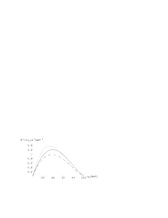
Figure 7: Spectrum of the emitted photons. The full line represents the full calculation including ${\cal{O}}((1/M)^{0})$ and ${\cal{O}}((1/M)^{1})$; the dashed line represents the result that contains only the ${\cal{O}}((1/M)^{0})$ contributions; the dotted line shows the result of [2, 5] with $g_{P}=6.6g_{A}$.

4 Discussion and Conclusions

A direct comparison of our calculation with the experimental data [1] is premature because we have not considered capture from the singlet and triplet hyperfine states separately, or capture from the $p\mu p$ molecular state. This also means that at this stage we cannot directly address the “$g_{P}$ problem” that arose from the TRIUMF data [1]. However, it is worthwhile to make the following remark. As one can see from Fig.7 our ChPT calculation gives for the spin-averaged $\mu p$-atomic RMC a photon spectrum that is slightly harder (by about 10% for $E_{\gamma}>$ 60 MeV) than what was obtained in [2, 5] with the use of the G-T value, $g_{P}=6.6g_{A}$. Meanwhile, as mentioned earlier, ChPT gives a value of $g_{P}$ consistent with $g_{P}=6.6g_{A}$ [14, 15]. Thus, there is a possibility that, even with the same value of $g_{P}$, a ChPT calculation gives a somewhat harder $\gamma$ spectrum than the conventional method. It remains to be seen to what extent such a difference in the $\gamma$ spectrum influences the $g_{P}$ value deduced from the experimental spectrum in the higher energy region. Of course, a more quantitative statement can be made only after a more detailed ChPT calculation becomes available in which the hyperfine states are separated and the $p\mu p$-molecular absorption is evaluated. We also remark that using relativistic kinematics, instead of the kinematic approximation employed in Eq.(16), softens the photon spectrum to a certain extent.

We repeat that the present calculation includes only up to the next-to-leading chiral order (NLO) contributions. The next-to-next-to-leading order (NNLO) calculations are obviously desirable. For this one must include the $\bar{\nu}=2$ chiral Lagrangian, ${\cal{L}}_{\pi}^{(2)}$ and ${\cal{L}}_{\pi N}^{(2)}$, and also loop corrections arising from ${\cal{L}}_{\pi}^{(0)}$ and ${\cal{L}}_{\pi N}^{(0)}$. The finite contributions from the loop diagrams would give momentum-dependent vertices, which would correspond to the form factors in the language of the phenomenological approach [2, 3, 5]. These contributions are probably small but it would be reassuring to check that explicitly. One problem in extending the present calculation to the next order is that, although the forms of ${\cal{L}}_{\pi}^{(2)}$ and ${\cal{L}}_{\pi N}^{(2)}$ have been determined [8, 18], some coefficients of the counter terms in ${\cal{L}}_{\pi N}^{(2)}$ still remain undetermined. On the other hand, chiral expansion for muon capture is characterized by the expansion parameter $m_{\mu}/M$, and is expected to converge reasonably rapidly. Indeed, in the case of OMC, where the $\nu=2$ calculation is much less involved, explicit evaluations [14, 15] show that the NNLO contributions amount only to a few percents. It is likely that, in the case of RMC as well, NNLO corrections modify our results only by a few percents. In this connection we also note that the formalism of Bernard et al.[10] used here does not contain the explicit $\Delta$ degree of freedom in contrast to the approaches of [16]. Although it is desirable to examine the importance of the $\Delta$, we relegate that to future studies. [After the completion of the present work we learned of the first attempt at an NNLO calculation by Ando and Min [19].]

References

[1]
G. Jonkmans et al., Phys. Rev. Lett. 77, (1996), 4512.
[2]
D.S. Beder and H.W. Fearing, Phys. Rev. D 35, (1987) 2130;
Phys. Rev. D 39, (1989) 3493.
[3]
G.K. Manacher and L. Wolfenstein, Phys. Rev. 116, (1959) 782.
[4]
G.I. Opat, Phys. Rev. 134, (1964) B428.
[5]
H.W. Fearing, Phys. Rev. C 21 (1980), 1951.
[6]
H.P.C. Rood and H.A. Tolhoek, Nucl. Phys. 70, (1965) 658;
R.S. Sloboda and H.W. Fearing, Nucl. Phys. A 340, (1980) 342;
H.W. Fearing and M.S. Welsh, Phys. Rev. C 46, (1992) 2077.
[7]
T.P. Gorringe et al., Phys. Rev. Lett. 72, (1994) 3472;
see also Proceedings of the 14th International
Conference on Particles and Nuclei,
ed. by C. Carlson and J. Domingo, World Scientific (1997).
[8]
J. Gasser and H. Leutwyler,
Ann. Phys. N.Y. 158, (1984) 142;
Nucl. Phys. B 250, (1985) 465.
[9]
For a review, see e.g.
G. Ecker, Prog. Part. Nucl. Phys. 35, (1995) 1.
[10]
For a review, see e.g.
V. Bernard, N. Kaiser and U.-G. Meissner,
Int. J. Mod. Phys. E4, (1995) 193.
[11]
C. Ordonez, L. Ray and U. van Kolck, Phys. Rev. Lett. 72, (1994) 1982;
Phys. Rev. C 53, (1996) 2086.
[12]
T.S. Park, D.-P. Min and M. Rho, Phys. Rep. 233, (1993) 341.
[13]
S.L. Adler and Y. Dothan, Phys. Rev. 151, (1966) 1267;
see also F. Christillin and S. Servadio, Nuovo Cimento 42, (1977) 165.
[14]
V. Bernard, N. Kaiser and U.-G. Meissner,
Phys. Rev. D 50, (1994) 6899.
[15]
H.W. Fearing, R. Lewis, N. Mobed and S. Scherer, hep-ph/9702394.
[16]
E. Jenkins and A.V. Manohar, Phys. Lett. B 255, (1991) 558;
Phys. Lett. B 259, (1991) 353;
T. Hemmert, B. Holstein and J. Kambor,
Phys. Lett. B 395, (1997) 89.
[17]
S. Weinberg, Phys. Lett. B 251, (1990) 288;
Nucl. Phys. B 363, (1991) 3; Phys. Lett. B 295, (1992) 114.
[18]
G. Ecker and M. Mojžiš, Phys. Lett. B 365, (1996) 312.