Propagation of Charm Quarks in Equilibrating Quark-Gluon Plasma

Abstract

We study the propagation of charm quarks, produced from the initial fusion of partons, in an equilibrating quark-gluon plasma which may be formed in the wake of relativistic collisions of gold nuclei. Initial conditions are taken from a self screened parton cascade model and the chemical equilibration is assumed to proceed via gluon multiplication and quark production. The energy loss suffered by the charm quarks is obtained by evaluating the drag force generated by the scattering with quarks and gluons in the medium. We find that the charm quarks may loose only about 10% of their initial energy in conditions likely to be attained at the Relativistic Heavy Ion Collider, while they may loose up to 40% of their energy while propagating in the plasma created at Large Hadron Collider. We discuss the implications for signals of quark gluon plasma.

PACS numbers: 12.38.Mh, 12.38.-t, 14.65.Dw, 25.75.-q

I INTRODUCTION

Relativistic heavy ion collisions are being studied with the intention of investigating the properties of ultradense, strongly interacting matter- quark-gluon plasma (QGP) [1]. The last several years have witnessed extensive theoretical efforts towards modeling these collisions. These studies suggest that at collider energies, one may visualize the nuclei as two clouds of valence and sea partons which pass through each other and interact [2]. The resulting partonic interactions may then produce a dense plasma of quarks and gluons. This plasma will expand and become cooler and more dilute. If quantum chromodynamics admits a first-order deconfinement or chiral phase transition, this plasma will pass through a mixed phase of quarks, gluons, and hadrons, before the hadrons loose thermal contact and stream freely towards the detectors.

One would like to understand several aspects of this evolution, viz., how does the initial partonic system evolve and how quickly does it attain kinetic equilibrium? How quickly, if at all, does it attain chemical equilibrium? And finally, how can we uncover the history of this evolution by studying the spectra of the produced particles, many of which may decouple from the interacting system only towards the end? These and related questions have been actively debated in recent times. Thus, it is believed by now that the large initial parton density may force many collisions among the partons in a very short time and lead to a kinetic equilibrium [3]. The question of chemical equilibration is more involved, as it depends on the time available to the system. If the time available is too short (3–5 fm/c), as at the energies ($\sqrt{s}\leq 100$ GeV/nucleon) accessible at the Relativistic Heavy Ion Collider (RHIC), the QGP will end its journey far away from chemical equilibrium. At the energies ($\sqrt{s}\leq 3$ TeV/nucleon) that will be achieved at the CERN Large Hadron Collider (LHC) this time could be large (more than 10 fm/$c$), driving the system very close to chemical equilibration [4, 5, 6, 7, 8], if there is only a longitudinal expansion. However, this time is also large enough to enable a rarefaction wave from the surface of the plasma to propagate to the center ($\tau_{s}\sim R_{T}/c_{s}$; $R_{T}$ is the transverse nuclear dimension and $c_{s}$ is the speed of sound), thus introducing large transverse velocity (gradients) in the system. The large transverse velocities may impede the chemical equilibration by introducing a faster cooling. The large velocity gradients may drive the system away from chemical equilibration by introducing an additional source of depletion of the number of partons [9] in a given fluid element.

Can we identify a probe for these rich details of the evolution? Dileptons and single photons have long been considered as useful probes of the various stages of the plasma as once produced they hardly ever interact and thus carry the details of the circumstances of their production. They are however produced at every stage of the collision and in an expanding system their number is obtained by an integration over the four-volume of the interaction zone. This moderates our estimate of the efficacy of these signals in several competing ways, as the space-time occupied by the hot plasma is small.

Consider the case of single photons. At very early times the temperature is rather high and we have a copious production of photons having a large transverse momentum. This should give us a reliable information about the initial conditions of the plasma. However, the transverse flow of the system is very moderate at early times. By the time the flow and other aspects of the QGP develop, the temperature would have dropped considerably and we have a large production of photons having smaller transverse momenta. However, the photons having a small transverse momentum will also be produced, and in much larger numbers, from the hadronic reactions and decays of vector mesons in the hadronic matter. Thus disentangling the development of the later stages of the evolution in the QGP would entail a very detailed understanding of the contributions of the hadronic matter. This is not trivial.

Next consider dileptons. Again, large mass dileptons, having their origin in early times, will be only marginally affected by these developments, e.g, the flow. The low-mass dileptons produced at later times will be affected strongly by the flow. However they will have, in addition to the contributions from the plasma, a large contribution from hadronic reactions. We shall be required to understand them in detail before we can confidently embark upon the task of deciphering the, more involved, development of the QGP, as it gets cool (see, e.g.,Ref, [9]). At the same time, there have been suggestions that correlated charm or bottom decay may give a large background to the dileptons from the QGP. We shall come back to this aspect later.

Why should we be so concerned about these late developments in the plasma? Firstly, it is not difficult to imagine that the detailed constitution of the hadronic matter should somehow reflect the state of chemical equilibration of the QGP at the time of the phase transition. Secondly, the transverse velocities, which may develop during the QGP phase will remain unaltered during the mixed phase, if such a phase is attained. The development of the transverse velocities should also be affected by the speed of sound, which may change rapidly as we approach the transition temperature. In the absence of transverse velocities, the mixed phase will last for a very long period of time [10]. And lastly, it is not at all clear that a non-equilibrated plasma will be adiabatically converted to hadronic matter, a scheme which is often invoked in hydrodynamic descriptions of the system.

In the present work we report on an investigation of the energy loss suffered by charm quarks in a chemically equilibrating plasma. This study has several interesting features. Firstly, heavy quarks are mostly produced from the initial fusion of partons in the colliding nucleons. If the initial temperature is high, at least charm quarks may also be produced at very early times (mostly from $gg\,\rightarrow\,c\overline{c}$, but also from $q\overline{q}\,\rightarrow\,c\overline{c}$). There is no production of charm quarks at later times and none in the hadronic matter. This makes them a good candidate for a probe of QGP. Again, as their number is not large, one can confidently ignore the reverse process ($c\overline{c}\,\rightarrow\,gg\,{\mathrm{or}}\,q\overline{q}$), where $q$ denotes one of the lighter quarks. (Of-course the associated production/suppression of $J/\Psi$ and $\Upsilon$ is a subject by itself.) The number of initially produced charm quarks (from fusion of primary partons) can be evaluated with a great degree of confidence using the perturbative QCD [11]. The thermally produced heavy quarks can also be estimated in terms of the temperatures and the fugacities during the early stage of evolution, when they are produced. Thus, the total number of c or b quarks gets frozen very early in the history of the collision. This can be of great help, as we are then left with the task of determining their $p_{T}$ distribution, whose details may reflect the developments in the plasma, but which is normalized to a given number of c (or b) quarks.

Now consider the central slice ($y=0$) of a collision which leads to production of a charm quark pair from initial fusion and QGP. The charm quarks will be produced on the order of a time scale $1/2m_{c}\,\simeq\,0.07$ fm/c, while the bottom quarks will similarly be produced over a time of $\sim 0.02$ fm/c. Thus, immediately upon production, these quarks will find themselves in a deconfined matter which is rapidly evolving, first towards kinetic equilibration and then towards chemical equilibration. The heavy quarks, as well as the light quarks and gluons will undergo scattering, with an interesting difference. The heavy quarks are not very likely to have a frequent and drastic change in their direction upon bombardment by massless quarks and gluons. These collisions will amount to a drag force. Svetitsky [12] has argued that this drag force is rather large and it will bring down the velocity of charm quarks down to thermal velocity very quickly.

In the present work we show that when we account for the non-equilibrium nature of the plasma, this drag force reduces considerably. In particular, we find that the charm quarks produced at the RHIC may loose only up to 10% of their initial momentum though at the LHC they may loose up to 40% of their initial momentum during their passage through the QGP phase of the matter.

The momenta of these quarks are likely to be reflected in the corresponding quantities of D mesons as the c quarks should pick up a light quark, which are in great abundance and hadronize. (One may add an interesting scenario, where the D mesons travel through a string of QGP droplets and loose further energy  [13].) Finally, they would scatter with hadronic matter before decoupling. Considering that $\sigma_{D\pi}\,\ll\,\sigma_{\pi\pi}$, e.g., it is most likely that the heavy mesons would decouple quickly from the hadronic phase.

There has been an attempt [14, 15] to estimate the change in the distribution of D mesons (open charm) by introducing a rate of energy loss $dE/dx\approx$ $-2$ GeV/fm for the charm and bottom quarks. We recall that this value was originally obtained [16] for very energetic quarks. For this reason, this estimate also derives a considerable contribution from the radiation of gluons. Charm quarks are very massive, and thus the radiation mechanism is absent [17] unless their energy is exceptionally high. We shall be concerned with charm quarks having a $p_{T}$ of a few GeV/c, in our study. For these energies, the drag force will come mostly from scatterings with light quarks and gluons [12] in a formulation which is equivalent to the treatment of Braaten and Thoma [18] for this purpose. We show in the present work that this energy loss can be very low for a chemically non-equilibrated plasma.

In the next Section, we briefly recall the initial conditions, and hydrodynamic and chemical evolution of the plasma in a (1+1) dimensional expansion. In Section III we give the formulation for drag force operating on the charm quarks in such an equilibrating plasma. We discuss our results in section IV. Finally, in section V we give a brief summary.

II INITIAL CONDITIONS, HYDRODYNAMIC EXPANSION, AND CHEMICAL EQUILIBRATION

It is quite clear that the fate of the heavy quarks will depend on the initial conditions and the history of evolution of the plasma. Fortunately, by now, a considerable progress has been achieved in our understanding of the parton cascades which develop in the wake of the collisions. Thus, in the recently formulated self-screened parton cascade [19] model early hard scatterings produce a medium which screens the longer ranged color fields associated with softer interactions. When two heavy nuclei collide at sufficiently high energy, the screening occurs on a length scale where perturbative QCD still applies. This approach yields predictions for the initial conditions of the forming QGP without the need for any ad-hoc momentum and virtuality cut-off parameters [2]. These calculations also show that the QGP likely to be formed in such collisions could be very hot and initially far from chemical equilibrium.

We assume that kinetic equilibrium has been achieved when the momenta of partons become locally isotropic. At the collider energies it has been estimated that, $\tau_{i}\approx 0.2-0.3$ fm/$c$ [3]. Beyond this point, further expansion is described by hydrodynamic equations and the chemical equilibration is governed by a set of master equations which are driven by the two-body reactions ($gg\,\leftrightarrow\,q\bar{q}$) and gluon multiplication and its inverse process, gluon fusion ($gg\,\leftrightarrow\,ggg$). The other (elastic) scatterings help maintain thermal equilibrium. The hot matter continues to expand and cools due to expansion and chemical equilibration. We shall somewhat arbitrarily terminate the evolution once the energy density reaches some critical value (here taken as $\epsilon_{f}=1.45$ GeV/fm³ [20]).

The expansion of the system is described by the equation for conservation of energy and momentum of an ideal fluid:

$$\partial_{\mu}T^{\mu\nu}=0\;,\qquad T^{\mu\nu}=(\epsilon+P)u^{\mu}u^{\nu}+Pg^{\mu\nu}\,,$$ (1)

where $\epsilon$ is the energy density and $P$ is the pressure measured in the frame comoving with the fluid. The four-velocity vector $u^{\mu}$ of the fluid satisfies the constraint $u^{2}=-1$. For a partially equilibrating plasma the distribution functions for gluons and quarks can be scaled through equilibrium distributions as

$$g_{i}(q,T,\lambda_{i})=\lambda_{i}g^{\mathrm{eq}}_{i}(q,T)\ \ ,$$ (2)

where $g^{\mathrm{eq}}_{i}(q,T)=({e^{\beta{u\cdot q}}\mp 1})^{-1}$ is the BE (FD) distributions for gluons (quarks), and $\lambda_{i}$ is the fugacity for parton species $i$, which describes the deviation from chemical equilibrium. This fugacity factor takes into account undersaturation of parton phase space density, $i.e.$, $0\leq\lambda_{i}\leq 1$. The equation of state for a partially equilibrated plasma of massless particles can be written as [4]

$$\epsilon=3P=\left[a_{2}\lambda_{g}+b_{2}\left(\lambda_{q}+\lambda_{\bar{q}}\right)\right]T^{4}\,,$$ (3)

where $a_{2}=8\pi^{2}/15$, $b_{2}=7\pi^{2}N_{f}/40$, $N_{f}\approx 2.5$ is the number of dynamical quark flavors. Now, the density of an equilibrating partonic system can be written as

$$n_{g}=\lambda_{g}\tilde{n}_{g},\qquad n_{q}=\lambda_{q}\tilde{n}_{q},$$ (4)

where $\tilde{n}_{k}$ is the equilibrium density for the parton species $k$:

$$\tilde{n}_{g}=\frac{16}{\pi^{2}}\zeta(3)T^{3}=a_{1}T^{3},$$ (5)

$$\tilde{n}_{q}=\frac{9}{2\pi^{2}}\zeta(3)N_{f}T^{3}=b_{1}T^{3}.$$ (6)

We further assume that $\lambda_{q}=\lambda_{\bar{q}}$. The equation of state (3) implies the speed of sound $c_{s}=1/\sqrt{3}$.

The master equations [4] for the dominant chemical reactions $gg\leftrightarrow ggg$ and $gg\leftrightarrow q\bar{q}$ are

$$\partial_{\mu}(n_{g}u^{\mu}) = n_{g}(R_{2\rightarrow 3}-R_{3\rightarrow 2})-(n_{g}R_{g\rightarrow q}-n_{q}R_{q\rightarrow g})\,,$$ (7)

$$\partial_{\mu}(n_{q}u^{\mu}) = \partial_{\mu}(n_{\bar{q}}u^{\mu})=n_{g}R_{g\rightarrow q}-n_{q}R_{q\rightarrow g},$$ (8)

in an obvious notation.

If we assume the system to undergo a purely longitudinal boost invariant expansion, (1) reduces to the well known relation [21]

$$\frac{d\epsilon}{d\tau}+\frac{\epsilon+P}{\tau}=0,$$ (9)

where $\tau$ is the proper time. This equation implies

$$\epsilon\,\tau^{4/3}=\,{\mathrm{const}.}$$ (10)

and the chemical master equations reduce to [4]

$$\frac{1}{\lambda_{g}}\frac{d\lambda_{g}}{d\tau}+\frac{3}{T}\frac{dT}{d\tau}+\frac{1}{\tau} = R_{3}(1-\lambda_{g})-2R_{2}\left(1-\frac{\lambda_{q}\lambda_{\bar{q}}}{\lambda_{g}^{2}}\right)\,,$$ (11)

$$\frac{1}{\lambda_{q}}\frac{d\lambda_{q}}{d\tau}+\frac{3}{T}\frac{dT}{d\tau}+\frac{1}{\tau} = R_{2}\frac{a_{1}}{b_{1}}\left(\frac{\lambda_{g}}{\lambda_{q}}-\frac{\lambda_{\bar{q}}}{\lambda_{g}}\right)\,,$$ (12)

which are then solved numerically for the fugacities with the initial conditions obtained from self screened parton cascade model [19]. We quote the rate constants $R_{2}$ and $R_{3}$ appearing in Eq. (8) for the sake of completeness [4];

$$R_{2} \approx 0.24N_{f}\alpha_{s}^{2}\lambda_{g}T\ln(1.65/\alpha_{s}\lambda_{g}),$$ (13)

$$R_{3} = 1.2\alpha_{s}^{2}T(2\lambda_{g}-\lambda_{g}^{2})^{1/2},$$ (14)

where the color Debye screening and the Landau - Pomeranchuk - Migdal effect suppressing the induced gluon radiation have been taken into account, explicitly.

III DIFFUSION OF HEAVY QUARKS IN QUARK GLUON PLASMA

The early results of parton cascade model [2] do indicate that the charm quarks which are produced from initial fusion in heavy ion collisions may have a transverse momentum distribution given by a power law, initially. With the passage of time, these distributions start evolving into an exponential shape, due to scattering with other partons, which is characteristic of a thermalized system of particles. Will these heavy quarks stay in thermal equilibrium, till the end of the QGP phase? For this we have to continue the cascading till the temperatures have dropped to $T_{c}$ or the energy density has become too low. The parton cascade model also includes all the effects like scatterings and radiation, if any, on the heavy quark. We shall report on such an effort in a future publication [22].

In the present work, we adopt the procedure developed by Svetitsky [12], where one visualizes the effect of partonic collisions as leading to a drag force. We first generalize the treatment of Svetitsky to a non-equilibrated plasma and then evaluate the time variation of the so-called drag and the diffusion coefficients, to see whether heavy quarks will actually stop and diffuse at RHIC and LHC energies.

We write the Boltzmann equation for the density $f({\mathbf{p}},t)$ for a heavy quark in phase space:

$$\frac{\partial}{\partial t}f({\mathbf{p}},t)=\left[\frac{\partial f}{\partial t}\right]_{\mathrm{collisions}}\,\,.$$ (15)

It is assumed that there is no external force acting on the heavy quark and that the phase space distribution $f$ does not depend on the position of the quark. The right hand side of Eq. (15) represents a collision integral given by,

$$R({\mathbf{p}},t) = \left[\frac{\partial f}{\partial t}\right]_{\mathrm{collisions}}\ \$$ (16)

$$= \int d^{3}k\left[w({\mathbf{p+k,k}})f({\mathbf{p+k}})-w({\mathbf{p,k}})f({\mathbf{p}})\right],$$ (17)

where $w({\mathbf{p,k}})$ is the rate of collisions which change the momentum of the charmed quark from $\mathbf{p}$ to ${\mathbf{p-k}}$. The Eq.(LABEL:colrate) can be written explicitly [12] as

$$R({\mathbf{p}},t) = {\frac{1}{2E_{\mathbf{p}}}}\int{\frac{d^{3}{\mathbf{q}}}{(2\pi)^{3}2E_{\mathbf{q}}}}\int{\frac{d^{3}{\mathbf{q}}^{\prime}}{(2\pi)^{3}2E_{{\mathbf{q}}^{\prime}}}}\int{\frac{d^{3}{\mathbf{p}}^{\prime}}{(2\pi)^{3}2E_{{\mathbf{p}}^{\prime}}}}$$ (19)

$$\times {\frac{1}{\gamma_{c}}}\sum|{\cal M}|^{2}(2\pi)^{4}\delta^{4}\left(p+q-p^{\prime}-q^{\prime}\right)$$ (20)

$$\times \left[f({\mathbf{p}^{\prime}})g({\mathbf{q}^{\prime}}){\tilde{g}}({\mathbf{q}})-f({\mathbf{p}})g({\mathbf{q}}){\tilde{g}}({\mathbf{q}^{\prime}})\right],$$ (21)

where ${\mathbf{p^{\prime}=p-k}}$, ${\mathbf{q^{\prime}=q+k}}$, and $\gamma_{c}$ is spin and color degeneracy of the charm quarks. In the above, $g$ represents the distribution for quarks or gluons approximated as Eq. (2), earlier. We have also introduced the Bose enhancement (Pauli suppression) factors, $\tilde{g}(q)=1\pm g(q)$ for gluons ( quarks)  [23]. The matrix elements $|{\cal M}|^{2}$ for elastic processes can be obtained from [24, 12].

We may further simplify the above by assuming soft scatterings according to Landau [25] to obtain,

$$R\approx\int d^{3}{\mathbf{k}}\left[{\mathbf{k}}\cdot{\frac{\partial}{\partial{\mathbf{p}}}}+{\frac{1}{2}}k_{i}k_{j}{\frac{\partial^{2}}{{\partial{p}_{i}}{\partial{p}_{j}}}}\right](wf).$$ (22)

Now Eq. (15) reduces to well known Fokker-Planck form

$${\frac{\partial f}{\partial t}}={\frac{\partial}{\partial{p_{i}}}}\left[A_{i}({\mathbf{p}})f+{\frac{\partial}{\partial{p_{j}}}}\left(B_{ij}({\mathbf{p}})f\right)\right],$$ (23)

where the kernels

$$A_{i} = \int d^{3}{\mathbf{k}}w({\mathbf{p,k}})k_{i}\ \ ,$$ (24)

$$B_{ij} = {\frac{1}{2}}\int d^{3}{\mathbf{k}}w({\mathbf{p,k}})k_{i}k_{j}\ \ ,$$ (25)

can be identified with the drag and diffusion coefficients, respectively, using the Langevin formalism [12]. In particular, $A_{i}$ and $B_{ij}$ are given by,

$$A_{i} = {\frac{1}{2E_{\mathbf{p}}}}\int{\frac{d^{3}{\mathbf{q}}}{(2\pi)^{3}2E_{\mathbf{q}}}}\int{\frac{d^{3}{\mathbf{q}}^{\prime}}{(2\pi)^{3}2E_{{\mathbf{q}}^{\prime}}}}\int{\frac{d^{3}{\mathbf{p}}^{\prime}}{(2\pi)^{3}2E_{{\mathbf{p}}^{\prime}}}}$$ (26)

$$\times {\frac{1}{\gamma_{c}}}\sum|{\cal M}|^{2}(2\pi)^{4}\delta^{4}\left(p+q-p^{\prime}-q^{\prime}\right)$$ (27)

$$\times g({\mathbf{q}}){\tilde{g}}({\mathbf{q}^{\prime}})\left[\left(p-p^{\prime}\right)_{i}\right]$$ (28)

$$\equiv \langle\!\langle\left(p-p^{\prime}\right)_{i}\rangle\!\rangle\ \ ,$$ (29)

$$B_{ij} = {\frac{1}{2}}\langle\!\langle\left(p^{\prime}-p\right)_{i}\left(p^{\prime}-p\right)_{j}\rangle\!\rangle\ \ .$$ (30)

We note that the Eqs. (29) and (30) depend only on ${\mathbf{p}}$, and thus we may write [12];

$$A_{i} = p_{i}A(p^{2})\ \ ,$$ (31)

$$B_{ij} = \left[\delta_{ij}-{\frac{p_{i}p_{j}}{p^{2}}}\right]B_{0}(p^{2})+{\frac{p_{i}p_{j}}{p^{2}}}B_{1}(p^{2})\ \ ,$$ (32)

where

$$A = \langle\!\langle 1\rangle\!\rangle-\langle\!\langle{\mathbf{p\cdot p^{\prime}}}\rangle\!\rangle/p^{2}\ \ ,$$ (34)

$$B_{0} = {\frac{1}{4}}\left[\langle\!\langle{p^{\prime}}^{2}\rangle\!\rangle-\langle\!\langle({\mathbf{p^{\prime}\cdot p}})^{2}\rangle\!\rangle/p^{2}\right]\ \ ,$$ (35)

$$B_{1} = {\frac{1}{2}}\left[\langle\!\langle({\mathbf{p^{\prime}\cdot p}})^{2}\rangle\!\rangle/p^{2}-2\langle\!\langle{\mathbf{p^{\prime}\cdot p}}\rangle\!\rangle+p^{2}\langle\!\langle 1\rangle\!\rangle\right].$$ (36)

The integrals appearing in the equations given above can be further simplified, by solving the kinematics in the center of mass frame of the colliding particles, so that we can write,

$$\langle\!\langle F(\mathbf{p^{\prime}})\rangle\!\rangle = {\frac{1}{512\pi^{4}\gamma_{c}}}{\frac{1}{E_{\mathbf{p}}}}\int_{0}^{\infty}q\ dq\int_{-1}^{1}d(\cos\chi)$$ (37)

$$\times {\frac{\sqrt{(s+m_{c}^{2}-m_{g(q)}^{2})^{2}-4sm_{c}^{2}}}{s}}\ g(E_{\mathbf{q}})$$ (38)

$$\times \int_{-1}^{1}d\cos{\theta_{\mathrm{c.m.}}}\sum|{\cal M}|^{2}\int_{0}^{2\pi}d\phi_{\mathrm{c.m.}}$$ (39)

$$\times e^{\beta E_{\mathbf{q}^{\prime}}}g(E_{\mathbf{q}^{\prime}})F(\mathbf{p^{\prime}})\ .$$ (40)

where and $s=(E_{\mathbf{p}}+E_{\mathbf{q}})^{2}-(\mathbf{p}+\mathbf{q})^{2}$, $E_{\mathbf{q^{\prime}}}=E_{\mathbf{q}}+E_{\mathbf{p}}-E_{\mathbf{p^{\prime}}}$ and $\mathbf{p}^{\prime}$ is a function of $\mathbf{p}$, $\mathbf{q}$ and $\theta_{\mathrm{c.m.}}$. Note that in addition to other differences due to the introduction of the mass of quarks and gluons (see later) and the quantum statistics, this expression differs [26] by a factor of 2 from the corresponding Eq. (3.6) of Ref.[12]. The quantum statistical correction for gluons employed here introduces a divergence as $q\rightarrow 0$ which is absent if we use a Boltzmann distribution for them. We have avoided this divergence [23] by using the thermal gluon mass;

$$m_{g}^{2}=\lambda_{g}\left(1+{\frac{N_{f}}{6}}\right){\frac{g^{2}T^{2}}{3}}\ \ ,$$ (41)

where $g$ is QCD coupling constant ($\alpha_{s}=g^{2}/4\pi$). In order to retain a certain degree of self-consistency, we have also used the thermal quark mass;

$$m_{q}^{2}=\left(\lambda_{g}+{\frac{\lambda_{q}}{2}}\right){\frac{g^{2}T^{2}}{9}}\ \ .$$ (42)

We thus correct these masses for the absence of chemical equilibrium.

We have also evaluated the integrals appearing in Eqs. (29) etc. by a direct Monte Carlo procedure, and the results were found to agree with the simplified expressions given above.

IV RESULTS

A Chemically Equilibrated Plasma

As a first step we show in Fig. 1(a) the variation of the drag coefficient $A$ with the momentum of the charm quark $p$ for a chemically equilibrated QGP at a temperature of 500 MeV. First of all, we note that the consequences of introducing the quantum statistics are quite small. We must comment on the difference between our results and those of Svetitsky [12] before proceeding. Firstly, we have used $\alpha_{s}=$ 0.3, instead of 0.6 used by Svetitsky. Secondly, we have used $N_{f}$, the number of flavors, as 2.5 instead of 2. Finally, we have have used the Debye screening mass $\mu=\mu_{D}=\sqrt{4\pi\alpha_{s}\lambda_{g}}\ T$ in the internal gluon propagator in the $t-$ channel exchange diagram, to remain consistent with the description used while evaluating the chemical evolution of the QGP. This is in addition to the numerical factor of 2 mentioned above. We have verified that reverting to the values used by Svetitsky, we reproduce the results of Ref. [12], but for the numerical factor of 2.

FIG. 1.: The drag ($A$) and the diffusion ($B_{0}$ and $B_{1}-B_{0}$) coefficients for charm quarks in a fully equilibrated quark gluon plasma at a temperature of 500 MeV. The solid curves give the results with the proper quantum statistics while the dashed curves give the results with the Boltzmann distribution.

We find that our result for the drag coefficient $A$ is a factor about three smaller than obtained by Svetitsky. (Note that the results scale with $\alpha_{s}^{2}$.) This will have an important consequence as we shall see later.

The momentum dependence of the diffusion coefficients $B_{0}$ and $B_{1}-B_{0}$ are shown in Figs. 1(b) & 1(c). While the general behavior remains similar to the results of Svetitsky, our values are smaller, due to the reasons given earlier.

FIG. 2.: The energy loss ($dE/dx$) of heavy quarks as a function of their momenta for $T$=0.5 GeV and $\alpha_{s}=0.3$.

The energy loss $dE/dx$ is related to the drag coefficient $A$;

$$\frac{dE}{dx}=-A(p^{2})p\ .$$ (43)

In Fig. 2 we have compared our results for the energy loss suffered by charm and bottom quarks with the results of Braaten and Thoma [18] and Bjorken [27] (adopted to the case of heavy quarks). Our results agree with those of Braaten and Thoma within 10%. We note that even a fully equilibrated plasma, whose temperature is kept fixed at 500 MeV, a charm quark having a momentum of 1–5 GeV will travel for almost 8–10 fm before coming to rest. The results would be completely different for a $dE/dx$ of $\approx$ $-$2 GeV/fm assumed in the studies reported in Ref. [14, 15]. We feel however that at exceptionally high energies, the additional mechanism of gluon radiation may enhance the energy loss. That should be of interest if we wish to study the propagation of a heavy quark jet in the QGP.

FIG. 3.: The temperature dependence of the drag ($A$) and the diffusion ($B_{0}$ and $B_{1}-B_{0}$) coefficients for charm quarks in a fully equilibrated quark gluon plasma. The results shown employ the proper quantum statistics for the gluon and the quark distributions.

The temperature dependence of the drag and the diffusion coefficients for a fully equilibrated QGP is shown in Figs. 3(a–c). We see that the drag coefficient drops rapidly with decline in temperature, so that a low temperature QGP hardly offers any resistance to the motion of massive quarks, whose final momentum will thus be decided by the time it spends in the very hot plasma.

B Results for Chemically Equilibrating Plasma at RHIC & LHC Energies

The results given so far are for a fully equilibrated plasma. We have already discussed that the plasma likely to be created in relativistic heavy ion collisions is far from chemical equilibrium. In Fig. 4(a) we give the evolution of the temperature and fugacities for the plasma likely to be created at RHIC, using the procedure disussed earlier. The appropriate drag and diffusion coefficients at any time $\tau$ operating on the heavy quark are obtained by accounting for the current fugacities and the temperature. In order to avoid confusion, we define

$$\alpha(p^{2},\tau)=A\left(p^{2},T(\tau),\lambda_{q}(\tau),\lambda_{g}(\tau)\right),$$ (44)

and similarly $\beta_{0}=B_{0}$, $\beta_{1}=B_{1}$. The time dependence of the drag and the diffusion coefficients for some typical values of the momenta are given in Figs. 4(b–d). We see that the drag and the diffusion coefficients are large only at the very early times (due to the high temperatures then) and drop rapidly as the plasma cools.

The corresponding results for the plasma created at the LHC energies are given in Figs. 5(a–d). We now see that the drag and the diffusion coefficients are a factor of $\approx$ 3 larger at any given time for the same momentum compared to the case at RHIC. Thus we see that the rapid cooling of the plasma and the small values of the fugacities ensure that the charm quarks will experience strong drag force only very early in their life both at the RHIC and the LHC. The force is also unlikely to cause a complete stopping and diffusion of the charm quarks.

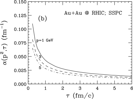
FIG. 4.: (a)The gluon fugacities ($\lambda_{g}$), the light quark fugacities ($\lambda_{q}$) and the temperature ($T$ in GeV) as a function of proper time ($\tau$) for a longitudinally expanding plasma likely to be created in Au+Au collisions at RHIC. (b–d) The variation of the drag ($\alpha$) and the diffusion ($\beta_{0}$ and $\beta_{1}-\beta_{0}$) coefficients with proper time ($\tau$) for different charm quark momenta.

The final momentum of the charm quark is likely to carry the effects of energy loss which in turn is affected by the cooling as well as the chemical evolution of the plasma. Thus for example, if we had a fully equilibrated QGP at the same initial temperatures as used here, then the drag at RHIC would be larger by more than a factor of three while at LHC energies, it would be large by a factor of more than two. Such large values for the drag force would ensure that at least the slower charm quarks produced at the LHC energies would come to rest soon after the creation and diffuse later in a manner discussed by Svetitsky. The final momenta of such charm quark (or D meson) would then be decided by the hadronization temperature.

FIG. 5.: Same as Fig. 4 for LHC energies.

In order to get an idea of the energy loss suffered by the charm quarks produced at RHIC and LHC, we have evaluated their final momentum after they travel through the plasma for the duration of the QGP phase.

Thus we write

$$\frac{d{\mathbf{p}}}{d\tau}=-\alpha(p^{2},\tau){\mathbf{p}}$$ (45)

and solve for ${\mathbf{p}}$ as a function of $\tau$. The results shown in Fig. 6 are very revealing. We find that by the time the QGP phase is over, the charm quark which was produced at the beginning of the collision would have lost up to 40% of its initial momentum at LHC energies, while at the RHIC, the energy loss may not exceed 10–12%.

FIG. 6.: The evolution of the charm quark momentum as a function of time in a partially equilibrated plasma at RHIC and LHC. The charm quarks are assumed to be produced with momenta of 1, 2, and 3 GeV at the time $\tau_{0}$.

C Distribution of Charm Quarks at RHIC & LHC

This has very interesting consequences. At RHIC energies, one may thus treat charm quark, almost as penetrating probes, which will provide information about the momentum distribution of the initially produced charm quark pairs. One can estimate the momentum distribution of initially produced charm pairs in a central Au+Au collisions by scaling the heavy-quark pair production cross-section in pp collisions as [28]

$${\frac{dN}{d^{2}p_{T}dy}}={\frac{1}{\pi}}T_{AB}(b=0){\frac{d\sigma}{dp^{2}_{T}dy}}$$ (46)

where $T_{AB}$ is the nuclear thickness factor. For central Au+Au collisions it’s value is 293.2 fm^-2 [29]. One may further approximate the thermal production of the charm quark pairs from Eq.(25) of Ref. [30]. The result of this study is shown in Fig. 7. One may obtain the “energy-loss corrected” distribution by decreasing the momenta by about 10%. This also implies that the dileptons from the annihilation of quarks would continue to remain buried under the leptons originating from the open charm decay, as originally inferred by authors of Ref. [11]. We may also add that as the charm quarks do not stop/diffuse at RHIC, they will not be affected by the transverse velocities which may develop during the QGP phase.

The situation is more complex at the LHC energies. Now the charm quarks can not be treated as penetrating probes. The results given in Fig. 8 correspond to situation when we treat them as penetrating probes, as in the early studies in this field. As most of the heavy quarks are produced very early in the collision, we can still get an idea of the final momentum distribution by decreasing the momenta in this figure by about 40%. This however may not be quite appropriate, as the charm quarks which have lost a large fraction of their initial momentum due to the drag force will start getting affected by the transverse flow of the QGP which can grow to large values at the LHC energies [9]. It is not clear that this situation can be accurately handled within a hydrodynamic description of the expansion. A more appropriate description could be the parton cascade model which includes collisions and even radiations from the charm quark. This work is under progress.

FIG. 7.: The momentum distribution of charm quarks for RHIC energies without energy loss.

FIG. 8.: The momentum distribution of charm quarks for LHC energies without energy loss.

All the same it is not difficult to imagine that the decrease in the slope of the $p_{T}$ distribution of the charm quarks is offset to a large extent by the flow velocity likely to develop at the LHC energies, and thus the dileptons from the plasma will perhaps remain buried under the open charm decay, at these energies as well, unless we look at too large masses.

V SUMMARY

In brief, we have obtained the drag and diffusion coefficients for charm quarks in a chemically equilibrating quark gluon plasma which may be produced at RHIC and LHC energies. Using a set of reasonable initial conditions, we find that a charm quark produced at the early stage of the collision may loose up to 10% of its momentum during the life-time of the QGP phase at the RHIC energies. This suggests that at the RHIC energies, dileptons originating from annihilation of quarks may remain buried under the background from open charm decay. The situation at LHC is more complex, as the charm quarks may loose up to 40% of the initial momentum. This could however be somewhat offset by the transverse flow of the QGP fluid, which could be large there. Further work, preferably within a parton cascade model is needed to settle some of these questions in a more definite manner, though we feel that even at the LHC energies, the dilepton signal may remain buried under the background from open charm decay. We may add that some recent works in this direction have used too large values for the energy loss, and arrived at results differing from our observations.

The small energy loss seen for heavy quarks in an equilibrating plasma could lead to a difference in the “quenching” of a heavy quark jet as compared to that of a gluonic jet. (Radiative loss of gluonic jets will presumably not be reduced, considerably, in an unequilibrated plasma.) This can be of great interest [31].

REFERENCES

- [1] J. W. Harris and B. Müller, Annu. Rev. Nucl. Part. Science 46, 71 (1996).
- [2] K. Geiger and B. Müller, Nucl. Phys. B369, 600 (1992); K. Geiger, Phys. Rep. 258, 376 (1995).
- [3] K. J. Eskola and X.-N. Wang, Phys. Rev. D49, 1284 (1994).
- [4] T. S. Biro, E. van Doorn, B. Müller, M. H. Thoma, and X. N. Wang, Phys. Rev. C 48, 1275 (1993).
- [5] K. Geiger and J. I. Kapusta, Phys. Rev. D 47, 4905 (1993).
- [6] K. Geiger, Phys. Rev. D 48, 4129 (1993).
- [7] J. Alam, S. Raha, and B. Sinha, Phys. Rev. Lett. 73, 1895 (1994).
- [8] X. M. H. Wong, Nucl. Phys. A 607, 442 (1996).
- [9] D. K. Srivastava, M. G. Mustafa, and B. Müller, Phys. Lett. B 396, 45 (1997); D. K. Srivastava, M. G. Mustafa, and B. Müller, nucl-th/9611041, Phys. Rev. C (in press).
- [10] H. von Gersdorff, L. McLerran, M. Kataja, and P. V. Ruuskanen, Phys. Rev. D 34, 794 (1986).
- [11] R. Vogt, B. V. Jacak, P. L. Mcgaughey, and P. V. Ruuskanen, Phys. Rev. D49, 3345 (1994); S. Gavin, P. L. McGaughey, P. V. Ruuskanen, and R. Vogt, Phys. Rev. C54, 2606 (1996).
- [12] B. Svetitsky, Phys. Rev. D 37, 2484 (1988).
- [13] B. Svetitsky, Phys. Lett. B 227, 450 (1989); B. Svetitsky, A. Uziel Phys. Rev. D 55, 2616 (1997).
- [14] E. Shuryak, Phys. Rev. C55, 961 (1997).
- [15] Z. Lin, R. Vogt, and X.-N. wang, nucl-th/9705006.
- [16] R. Baier, Yu. L. Dokshitzer, S. Peigne and D. Schiff, Phys. Lett. B 345, 277 (1995).
- [17] R. Baier (Private communication).
- [18] E. Braaten and M. H. Thoma, Phys. Rev. D 44, R2625 (1991).
- [19] K. J. Eskola, B. Müller, and X. N. Wang, Phys. Lett. B 374, 20 (1996).
- [20] 1.46 GeV/fm3 corresponds to the energy density for a fully equilibrated QGP at 160 MeV.
- [21] J. D. Bjorken, Phys. Rev. D 27, 140 (1983).
- [22] K. Geiger and D. K. Srivastava, under preparation.
- [23] D. Levin-Plotnik, M. Sc. Thesis, Tel-Aviv University (unpublished).
- [24] B. L. Combridge, Nucl. Phys. B 151, 429 (1979).
- [25] L. D. Landau, Zh. Eksp. Teor. Fiz. 7, 203 (1937), translated in Collected Papers of L. D. Landau, D. ter Harr, ed. (Pergamon, New York, 1981).
- [26] We have checked this with the author of Ref. [12]. We thank him for rechecking this aspect.
- [27] J. D. Bjorken, Fermilab Report No. PUB-82/59-THY (unpublished).
- [28] P. L. McGaughey, E. Quack, P. V. Ruuskanen, R. Vogt and X.-N. Wang, Int. J. Mod. Phys. A 10, 2999 (1995).
- [29] K. J. Eskola, R. Vogt and X.-N. Wang, Int. J. Mod. Phys. A 10, 3087 (1995).
- [30] P. Levai, B. Müller, and X.-N. Wang, Phys. Rev. C 51, 3326 (1995).
- [31] M. H. Thoma (Private communication).