A letter of intent for an experiment to measure $\nu_{\mu}\rightarrow\nu_{e}$ oscillations and $\nu_{\mu}$ disappearance at the Fermilab Booster: BooNE

1 Executive Summary

The MiniBooNE experiment will be capable of observing both $\nu_{\mu}\rightarrow\nu_{e}$ appearance and $\nu_{\mu}$ disappearance. In addition, the experiment will be able to measure $\Delta m^{2}$ and $\sin^{2}2\theta$ and search for CP violation in the lepton sector. By using the phototubes and electronics from LSND, the detector cost is estimated to be $1.6M and we estimate that the neutrino beam line would cost $3M.

This Letter of Intent describes a search for neutrino oscillations motivated by the LSND observation, which has been interpreted as $\bar{\nu}_{\mu}\rightarrow\bar{\nu}_{e}$, and by the atmospheric neutrino deficit which may result from $\nu_{\mu}$ oscillations. The BooNE (Booster Neutrino Experiment) program will have two phases. The first phase, MiniBooNE, is a single detector experiment designed to:

• Obtain $\sim 400$ events per Snowmass-year ($1\times 10^{7}$ s) if the LSND signal is due to $\nu_{\mu}\rightarrow\nu_{e}$ oscillations.

• Extend the search for $\nu_{\mu}\rightarrow\nu_{e}$ oscillations approximately one order of magnitude in $\Delta m^{2}$ beyond what has been studied previously if no signal is observed.

• Search for $\nu_{\mu}$ disappearance, to address the atmospheric neutrino deficit, through the suppression of the expected 50,000 $\nu_{\mu}C\rightarrow\mu+X$ events per Snowmass-year.

• Test CP-violation in the lepton sector if oscillations are observed by running with separate $\nu_{\mu}$ and $\bar{\nu}_{\mu}$ beams.

The second phase of the experiment introduces a second detector, with the goals of:

• Accurately measuring the $\Delta m^{2}$ and $\sin^{2}2\theta$ parameters of observed oscillations.

• Determining the CP violation parameters in the lepton sector.

The MiniBooNE experiment (phase 1) would begin taking data in 2001. By using phototubes and electronics from the LSND experiment, the MiniBooNE Detector is relatively inexpensive, $1.6 M, and able to be constructed on a short time scale. The detector would consist of a double-wall cylindrical tank which is 11 m in diameter and 11 m high. The inner tank would be covered on the inside by 1220 8-inch phototubes (10% coverage) and filled with 600 t of mineral oil, resulting in a 400 t fiducial volume. The volume between the tanks would be filled with scintillator oil to serve as a veto shield for identifying particles both entering and leaving the detector. The detector would be located 1000 m from a neutrino source.

The neutrino beam constructed using the 8 GeV proton Booster at FNAL would service both phases of the experiment. The neutrino beam line would consist of a target followed by a focusing system and a $\sim$30 m long pion decay volume. The low energy, high intensity and 1 $\mu$s time-structure of a neutrino beam produced from the booster beam are ideal for this experiment. The sensitivities discussed in this Letter of Intent assume the experiment receives 5 Hz of protons in one Snowmass-year. The cost of this beam line is expected to be $3 M.

This Booster experiment is compatible with the Fermilab collider or the fixed-target MI programs. The FNAL Booster is capable of running at 15 Hz ($5\times 10^{12}$ protons per pulse), or 30 Booster batches per 2 s Main Injector Cycle. The antiproton stacking requires only 6 Booster batches at the start of the Main Injector cycle. In principle, this means the BooNE beam line could receive 12 Hz, well above the expectation on which our sensitivities are based.

The BooNE experiments represent an opportunity to resolve two outstanding neutrino oscillation questions on a short-time scale. Within the upcoming five years, no existing or approved experiments will be able to address conclusively the LSND signal region. Also, there are no accelerator-based experiments within this time scale that can prove conclusively that oscillations are the source of the atmospheric neutrino deficit. Thus BooNE represents an important and unique addition to the Fermilab program.

A formal proposal for this experiment will be submitted to the Fermilab Physics Advisory Committee in the autumn of 1997.

2 Introduction

The MiniBooNE experiment is motivated by the evidence for neutrino oscillations from the LSND and atmospheric neutrino experiments. The detector will be similar to that in the LSND experiment and will be located 1000m from a neutrino beam line fed by the 8 GeV proton Booster.

2.1 Motivation

This experiment is motivated by two important pieces of evidence for neutrino oscillations. The first is the observation of events by the LSND collaboration that are consistent with $\bar{\nu}_{\mu}\rightarrow\bar{\nu}_{e}$ oscillations. The second is the observed deficit of atmospheric neutrinos which may be attributed to $\nu_{\mu}$ disappearance through oscillations. Here we briefly review these results and the expectation for what MiniBooNE can contribute. Chapter 3 provides further details on these results and other experimental evidence for neutrino oscillations.

The LSND experiment at Los Alamos has reported evidence[1] for $\bar{\nu}_{\mu}\rightarrow\bar{\nu}_{e}$ oscillations with an oscillation probability of $\sim 0.3\%$. The allowed values of $\Delta m^{2}$ and $\sin^{2}2\theta$ corresponding to this oscillation probability are indicated in Fig. 1 by the grey region. Previous oscillation searches have not seen oscillations in the LSND allowed region for $\Delta m^{2}>4$ eV², as shown in Fig. 1. This isolates the most favored region at low $\Delta m^{2}$. LSND also is able to search for $\nu_{\mu}\rightarrow\nu_{e}$ oscillations using $\pi^{+}$ that decay in flight in the beam stop. This decay-in-flight oscillation search has different backgrounds and systematics than the decay-at-rest search, and the presence of an excess that is consistent with the decay-at-rest search provides additional evidence that the LSND results are due to neutrino oscillations.

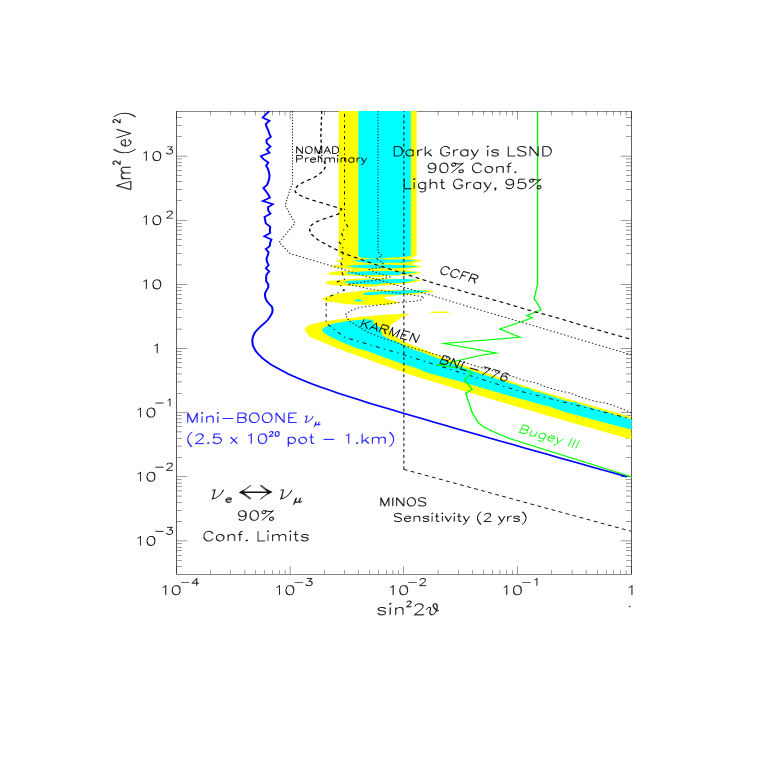
Figure 1: 90% C.L. limit expected for MiniBooNE for $\nu_{\mu}\rightarrow\nu_{e}$ appearance after one year of running, including 10% systematic error, if LSND signal is not observed (solid line). Summary of results from past experiments and expectations for the future MINOS experiment are also shown.

If the LSND signal is due to neutrino oscillations, MiniBooNE expects between 100 and 400 events per Snowmass-year, depending on the $\Delta m^{2}$ and $\sin^{2}2\theta$ of the oscillation, outside of the regions ruled out by previous experiments. The expectations are shown in Fig.  2 (solid line). The MiniBooNE systematics are significantly different to the LSND experiment. Thus MiniBooNE will be able to verify or disprove the LSND result. The full BooNE two-detector system will then accurately measure the oscillation parameters.

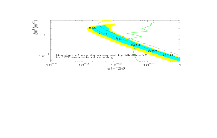
Figure 2: If LSND signal is observed, this plot shows the number of events expected in 1 Snowmass-year of running for MiniBooNE for the low $\Delta m^{2}$ favored region for LSND (shaded). Lines indicate regions excluded by past experiments (see Fig. 1).

If the LSND signal is not observed by MiniBooNE, then the expected sensitivity is shown in Fig. 1. This experiment extends approximately an order of magnitude in $\Delta m^{2}$ beyond previous limits.

The second important hint for neutrino oscillations comes from experiments which indicate a deficit of muon neutrinos from cosmic ray production in the atmosphere. The Kamioka and IMB experiments[5, 6] determined the ratio of $\nu_{\mu}/\nu_{e}$ to be only about 60% of the theoretically expected ratio for neutrino energies below $\sim$1 GeV, independent of the visible energy of the charged lepton and the projected zenith angle of the atmospheric neutrinos. Interpreting the shortfall as arising from oscillation of muon neutrinos requires a large mixing angle ($\sin^{2}2\theta\sim 0.5$) and a $\Delta m^{2}>10^{-3}$ eV². The atmospheric problem can be attributed to either $\nu_{\mu}\rightarrow\nu_{e}$ or $\nu_{\mu}\rightarrow\nu_{\tau}$ oscillations. Because the Bugey result, shown in Fig.  1, excludes the atmospheric neutrino deficit region, $\nu_{\mu}\rightarrow\nu_{\tau}$ oscillations are considered to be the likely candidate.

Upper limits on the possible $\Delta m^{2}$ range come from previous accelerator-based experiments and the zenith angle dependence of the atmospheric neutrino deficit. The CDHS search for $\nu_{\mu}$ disappearance indicates $\Delta m^{2}<0.4$ eV². The Kamioka group has observed a zenith angle dependence of the high energy (greater than 1 GeV) atmospheric neutrino sample[7] which indicates that $\Delta m^{2}~{}<<0.5$ eV² (Kamioka prefers a $\Delta m^{2}\sim 10^{-2}$ eV²), although the uncertainties are large. However a recent publication from the IMB collaboration[8] reports no zenith angle dependence. Also, preliminary data from the Super Kamiokanda collaboration shows a zenith angle distribution that is consistent with being flat and, in any case, with less angular dependence (see section 3.4).

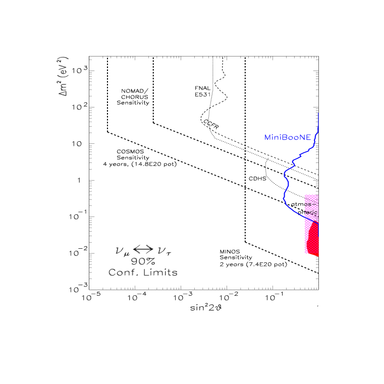
Figure 3: Summary of results from past experiments (narrow, dashed and dotted), future approved experiments (wide, dashed) and 90% C.L. limit expected for MiniBooNE (solid) for $\nu_{\mu}$ disappearance after one year of running at 1 km. Solid region indicates the favored region for the atmospheric neutrino deficit from the Kamioka experiment. A result from Kamiokanda indicating no zenith angle dependence extends the favored region to higher $\Delta m^{2}$ as indicated by the hatched region.

Figure 3 shows an overview of past experiments (narrow dashed and dotted lines) and expectations for future approved experiments (wide dashed lines) for $\nu_{\mu}\rightarrow\nu_{\tau}$ searches. In light of the changing situation concerning the zenith angle dependence, Fig. 3 shows the allowed region if there is a zenith angle dependence (solid) and if there is no dependence (hatched). In the higher $\Delta m^{2}$ scenario, MiniBooNE (solid line) can address the atmospheric neutrino oscillation question by searching for $\nu_{\mu}$ disappearance. MiniBooNE is sensitive to variations in the flux with energy that are consistent with oscillations. Statistical and 10% systematic errors were included in this determination. Issues relating to the precision of the $\nu_{\mu}$ disappearance search in MiniBooNE are discussed in section 9.4.

The case where the $\Delta m^{2}$ values from atmospheric neutrino experiments are compatible with LSND provides a useful example of a three-generation mixing formalism which may be applied to explain the present pieces of evidence for neutrino oscillations. If $\Delta m^{2}$ for $\nu_{\mu}\rightarrow\nu_{e}$ from LSND is approximately the same as $\Delta m^{2}$ from $\nu_{\mu}\rightarrow\nu_{\tau}$ in the atmospheric case, then three-generation mixing models[3] with only one dominant mass value for the mass eigenstates, i.e., $m_{3}\gg m_{1}\approx m_{2}$, apply. In this case, the LSND result is explained via $\nu_{\mu}\rightarrow\nu_{3}\rightarrow\nu_{e}$ while the atmospheric result is explained through $\nu_{\mu}\rightarrow\nu_{3}\rightarrow\nu_{\tau}$. This and other examples of three generation mixing models are discussed in section 3.5.

MiniBooNE is an experiment which can and should be done on a short time scale. Construction of MiniBooNE can be completed by 2001, as discussed in sections 5 and 6. Thus the data-taking and analysis presented above is expected to be completed by 2003. Within the next five years there are no other accelerator experiments that can address fully the oscillation issues described above. The KARMEN experiment, which is presently running at the ISIS facility with a segmented liquid scintillator detector, may have sufficient statistics to verify the LSND signal with similar systematics to LSND if $\Delta m^{2}$ is greater than 1 eV²; however, KARMEN will have difficulty proving that the signals are due to neutrino oscillations because of similar systematics.[4] In the low $\Delta m^{2}$ region, KARMEN will not have sufficient statistics to verify fully the LSND result.[4] Super Kamiokanda will greatly refine the atmospheric neutrino deficit measurement using past techniques. While this is quite important, an experiment such as MiniBooNE, with very different systematics is required to verify that the deficit is due to neutrino oscillations. Finally, the MINOS experiment is not scheduled to begin running until 2003 and requires two years to obtain the sensitivity indicated on Figs.  1 and  3. Thus, MiniBooNE fills an important gap within the global neutrino program. It should be noted that there are competitive proposals in preparation for submission to CERN. Therefore, it is important that Fermilab seize the initiative in pursuing accelerator-based oscillation physics within the next decade.

2.2 Neutrino Beam and Detector

Discussion with FNAL staff and management indicate that the Booster is capable of providing an additional 5 pulses per second at $\sim 5\times 10^{12}$ protons per 1 $\mu$ sec pulse at 8 GeV beyond the requirements for antiproton stacking. As 2 GeV pion production is copious from an 8 GeV beam, we propose building a focusing system capable of producing a parallel beam of pions centered on 2 GeV/c. This beam has a relatively short decay length of 30 m, so that the fraction of $\nu_{e}$ in the beam from the $\pi\rightarrow\mu\rightarrow e$ decay chain is kept at a low level, as these $\nu_{e}$ are a basic background for the appearance measurement. The focusing system will be capable of operation in either positive or negative polarity. The positive polarity yields a higher neutrino flux, although the $\nu_{e}$ background from kaon decays is lower for the negative polarity. The duty factor of the Booster beam with single turn extraction makes cosmic ray background manageable and makes the data acquisition problem much simpler than for LSND. The decay region is designed to reduce the $\nu_{e}$ contribution from kaon and muon decays. Particle production in the beam line is monitored using similar systems to those in the NuTeV experiment. The beam design is described in Chapter 5.

We propose building a 600 ton detector located at 1000 m from the neutrino source. The detector will be capable of measuring the $\nu_{e}$ and $\nu_{\mu}$ energy spectra though quasi elastic scattering as described in Chapter 7, and the event energy distribution in the detector will allow the determination of the neutrino oscillation parameters. The detector is very similar to that in the LSND experiment, allowing transfer of analysis expertise, particularly in the area of particle identification.

3 Status of Neutrino Oscillation Experiments

Evidence for neutrino oscillations come from the solar neutrino experiments, the atmospheric neutrino experiments, and the LSND experiment. These results can be interpreted within three-generation neutrino mixing models. Although future experiments are planned, MiniBooNE fulfills a unique niche in addressing the present evidence for neutrino oscillations.

3.1 Neutrino Oscillation Formalism

If neutrinos have mass, it is likely that the interaction responsible for mass will have eigenstates which are different from the weak eigenstates that are associated with weak decays. In this model, the weak eigenstates are mixtures of the mass eigenstates and lepton number is not strictly conserved. A pure flavor (weak) eigenstate born through a weak decay will oscillate into other flavors as the state propagates in space. This oscillation is due to the fact that each of the mass eigenstate components propagates with a different phase if the masses are different, $\Delta m^{2}=\left|m_{2}^{2}-m_{1}^{2}\right|>0$. The most general form for 3-component oscillations is

$$\left(\begin{array}[]{l}\nu_{e}\\ \nu_{\mu}\\ \nu_{\tau}\end{array}\right)=\left(\begin{array}[]{lll}U_{e1}&U_{e2}&U_{e3}\\ U_{\mu 1}&U_{\mu 2}&U_{\mu 3}\\ U_{\tau 1}&U_{\tau 2}&U_{\tau 3}\end{array}\right)\left(\begin{array}[]{l}\nu_{1}\\ \nu_{2}\\ \nu_{3}\end{array}\right)$$

This formalism is analogous to the quark sector, where strong and weak eigenstates are not identical and the resultant mixing is described conventionally by a unitary mixing matrix. The oscillation probability is then:

$${\rm Prob}\left(\nu_{\alpha}\rightarrow\nu_{\beta}\right)=\delta_{\alpha\beta}-4\sum\limits_{j>\,i}U_{\alpha\,i}U_{\beta\,i}U^{*}_{\alpha\,\,j}U^{*}_{\beta\,\,j}\sin^{2}\left(\frac{1.27\;\Delta m_{i\,j}^{2}\left({\rm eV^{2}}\right)\,L\left({\rm km}\right)}{E_{\nu}\left({\rm GeV}\right)}\right)$$ (1)

where $\Delta m_{i\,j}^{2}=\left|m_{i}^{2}-m_{j}^{2}\right|$ . Note that there are three different $\Delta m^{2}$ (although only two are independent) and three different mixing angles. The oscillation probability also depends upon the length, L, from the source and neutrino energy, E_ν.

Although in general there will be mixing among all three flavors of neutrinos, two-generation mixing is often assumed for simplicity. If the the mass scales are quite different ($m_{3}>>m_{2}>>m_{1}$ for example), then the oscillation phenomena tend to decouple and the two-generation mixing model is a good approximation in limited regions. In this case, each transition can be described by a two-generation mixing equation:

$$P=\sin^{2}2\theta~{}\sin^{2}(1.27\Delta m^{2}~{}L/E_{\nu})$$ (2)

where $\theta$ is the mixing angle. However, it is possible that experimental results interpreted within the two-generation mixing formalism may indicate very different $\Delta m^{2}~{}$ scales with quite different apparent strengths for the same oscillation. This is because, as is evident from equation 1, multiple terms involving different mixing strengths and $\Delta m^{2}$ values contribute to the transition probability for $\nu_{\alpha}\rightarrow\nu_{\beta}$.

3.2 LSND Results

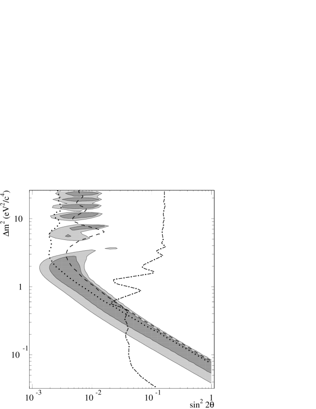
Figure 4: Allowed regions in the $\Delta m^{2}~{}$ vs $\sin^{2}2\theta~{}$ parameter space from the LSND $\bar{\nu}_{\mu}\rightarrow\bar{\nu}_{e}$ appearance experiment. Also shown are $90\%$ C.L. limits from KARMEN at ISIS (dashed curve), E776 at BNL (dotted curve), and the Bugey reactor experiment (dot-dashed curve).

Figure 5: Allowed regions in the $\Delta m^{2}~{}$ vs $\sin^{2}2\theta~{}$ parameter space from the LSND $\nu_{\mu}\rightarrow\nu_{e}$ (solid curve) and $\bar{\nu}_{\mu}\rightarrow\bar{\nu}_{e}$ (dashed curve) appearance experiments.

The LSND accelerator experiment uses a detector composed of 167 tons of dilute liquid scintillator placed 30 m from the beam stop of the LAMPF 800 MeV proton beam.[1] Neutrinos are produced from stopped $\pi^{+}\rightarrow\mu^{+}\nu_{\mu}$ and $\mu^{+}\rightarrow e^{+}\nu_{e}\bar{\nu}_{\mu}$ decays. At the detector the $\bar{\nu}_{e}$ are detected by $\bar{\nu}_{e}p\rightarrow e^{+}n$, and the neutron is then captured producing a 2.2 MeV gamma. The experiment has reported evidence[1] for $\bar{\nu}_{\mu}\rightarrow\bar{\nu}_{e}$ oscillations by observing $51.0_{-19.5}^{+20.2}\pm 8.0$ $\bar{\nu}_{e}$ events above background. This corresponds to an oscillation probability of Prob$\left(\bar{\nu}_{\mu}\rightarrow\bar{\nu}_{e}\right)=(0.31\pm 0.11\pm 0.05)\%$ and with an oscillation parameter allowed region shown in Fig. 4. Due to the low 800 MeV proton energy of the LAMPF beam, the neutrino backgrounds are quite small and well understood. The largest background is from $\mu^{-}$ decay at rest in the beam stop, which is suppressed by a factor of $7\times 10^{-4}$ relative to $\mu^{+}$ decay at rest. The suppression results from the following three factors: the ratio of $\pi^{-}$ to $\pi^{+}$ (0.12) times the probability that the $\pi^{-}$ decays in flight (0.05) times the probability that the $\mu^{-}$ decays at rest (0.12).

The LSND signal is strengthened by a complementary $\nu_{\mu}\rightarrow\nu_{e}$ oscillation search,[2] which has completely different systematics and backgrounds than the $\bar{\nu}_{\mu}\rightarrow\bar{\nu}_{e}$ oscillation search. The neutrinos for this search come from pion decay in flight and are of higher energies than those produced by stopped muons. Thus it is interesting that the decay in flight analysis does show a signal, although of lesser significance, which indicates the same favored regions of $\Delta m^{2}$ and $\sin^{2}2\theta$ (see Fig. 5) as the decay at rest analysis. A global analysis of the decay-in-flight and decay-at-rest data is in progress.

3.3 Solar Neutrino Experiments

Since the first observation of $\nu_{e}$ interactions in a Cl target in the Homestake mine by Davis and collaborators,[9] three additional experiments have measured solar neutrino interactions and have determined that there are fewer neutrinos from the sun than are expected from the Standard Solar Model. There have been two experiments using Ga as target, GALLEX and SAGE, and the experiment at Kamioka in which neutrinos were scattered from electrons in water. The Ga experiments[10] have the lowest energy threshold, while Kamioka[11] is limited by the $\sim 7\,{\rm MeV}$ detection energy threshold for electrons. Hata and Langacker published[12] a thorough analysis of these data two years ago. They considered experimental errors in detail as well as possible variations in the Standard Solar Model which is used to predict the flux of neutrinos that is expected from the sun in the absence of neutrino oscillations. Each of the experiments is sensitive to different parts of the neutrino spectrum. These sensitivities are shown in Table 1 using the Standard Solar Model of Bahcall and Pinsonneault[13]. The experimental results are shown in Table 2, where it is clearly seen that the measured solar neutrino flux is below the prediction of the Standard Solar Model.

Table 1: Sensitivities of the three types of solar neutrino experiments on the expected reactions in the Standard Solar Model.

	Kamioka	Homestake	GALLEX/SAGE
pp			0.538
7Be I			0.009
7Be II		0.150	0.264
8Be	1	0.775	0.105
pep		0.025	0.024
${}^{1}3$N		0.013	0.023
${}^{1}5$O		0.038	0.037

Table 2: The measured rate from the three types of solar neutrino experiments compared to the Standard Solar Model.

Experiment	Rate
GALLEX/SAGE	$0.62\pm 0.10$
Homestake	$0.29\pm 0.03$
Kamioka	$0.51\pm 0.07$

Hata and Langacker conclude that the experimental data cannot be explained by variations in solar physics and that neutrino oscillations are strongly favored. Also, resonant transformation of $\nu_{e}$ to other flavors through the MSW effect is preferred, leading to the allowed region in the $\Delta m^{2}~{}$ - $\sin^{2}2\theta~{}$ parameter space shown in Fig. 6. Although we have stressed that three generations of neutrinos must be considered in general, that need not apply to the solar neutrino discussion as long as the masses $m_{1}$, $m_{2}$, $m_{3}$ are described by $m_{3}>>m_{2},m_{1}$. As the small mixing solution is favored, a value for $\theta_{12}$ of about $3\times 10^{-2}$ is implied. It is worth emphasizing that these data have been gathered over an extended period of time and that many systematic checks have been performed. Furthermore, the solar model is very much constrained by the solar luminosity, particularly in the case of the Gallium reaction. The Kamioka result should be confirmed by Super Kamioka in the near future with significantly better statistics. Also, the neutrino oscillation hypothesis will be tested by the SNO experiment, which will measure both charged and neutral current solar neutrino interactions. Overall, the solar neutrino experimental observation appears firm, although uncertainties in solar dynamics are still a cause for concern.

Figure 6: Allowed regions in the $\Delta m^{2}~{}$ vs $\sin^{2}2\theta~{}$ parameter space from the four solar neutrino experiments.

3.4 Atmospheric Neutrino Experiments

Cosmic rays interacting in the upper atmosphere produce pions that decay into muons and neutrinos. In approximate terms, this decay chain produces two muon neutrinos for each electron neutrino. Charged-current reactions from these neutrinos have been observed in a number of detectors. The sensitivity of these detectors to electrons and muons varies over the observed energy range, and so the experiments depend on a Monte Carlo simulation to determine the relative efficiencies. For example, electron events are mostly contained in the detector, while muon events have longer range and escape the detector at the higher energies. The experiments report the observed ratio of muon to electron events divided by the ratio of events calculated in a Monte Carlo simulation. The experiments also model the absolute neutrino flux. A recent summary of the experimental situation is discussed by Gaisser and Goodman[14] and shown in Table 3. Several experiments measure the ratio of observed events to expected events to be less than one. For Kamioka the data is divided into low and high energy samples. The low energy events have a muon (with energy typically less than 1 GeV) that is contained in the detector. Muons are identified in two ways by both Kamioka and IMB. The first way involves identification of the $\check{\rm C}$erenkov ring, which is significantly different for electrons and muons. (There is also a significant difference between the efficiency for detection of electrons and muons, but this is presumably in the detector simulation.) The second method uses the fact that muons that stop in H₂O usually decay, allowing the observation of decay Michel electrons to facilitate identification of the muon. The ratio is consistent using both methods of identification.

Table 3: Ratio of $\nu_{\mu}$ to $\nu_{e}$ observed events divided by the ratio of expected events for the different atmospheric oscillation experiments.

Experiment	Exposure	Flavor Ratio
	kT - year	$\mu$ / e
IMB1	3.8	$0.68\pm 0.08$
Kamioka Ring	7.7	$0.60\pm 0.06$
Kamioka Decay		$0.69\pm 0.06$
IMB - 3 Ring	7.7	$0.54\pm 0.05$
IMB - 3 Decay		$0.64\pm 0.07$
Frejus Contained	2.0	$0.87\pm 0.13$
Soudan	1.0	$0.64\pm 0.19$
NUSEX	0.5	$0.99\pm 0.29$

For the fully contained events the muon energy is sufficiently low that the cross section is over predicted by the Fermi gas model[15] used by all experiments. This is a valid concern but seems unlikely to explain the large and persistent effect observed. Moreover, this problem should not afflict the second sample of partially contained events for which the energy is typically $\sim 5\,{\rm GeV}$. It is our view, and that of the experimenters, that the $\nu_{\mu}/\nu_{e}$ ratio is suppressed, although some systematic effects are still to be understood.

Figure 7: Zenith-angle distributions from the Kamioka experiment for (a) the electron-like events and (b) the muon-like events. The circles with error bars show the data and the histogram the MC simulation (without oscillations).

Figure 8: Zenith-angle distribution from the Kamioka experiment of $(\mu/e)_{data}/(\mu/e)_{MC}$. The circles with error bars show the data. Also shown are the expectations from the MC simulations with neutrino oscillations for parameter sets $(\Delta m^{2},\sin^{2}2\theta)$ corresponding to the best-fit values to the multi-GeV data for $\nu_{\mu}\rightarrow\nu_{e}$ (($1.8\times 10^{-2}$ eV², 1.0), dashes) and $\nu_{\mu}\rightarrow\nu_{\tau}$ (($1.6\times 10^{-2}$ eV², 1.0), dots) oscillations.

The Kamioka group has reported a zenith angle dependence of the apparent atmospheric neutrino deficit[7], based on their examination of higher energy atmospheric neutrino events (visible energy greater than 1.3 GeV and average energy equal to 6 GeV). In this instance the observed $\nu_{\mu}/\nu_{e}$ ratio was $0.57\pm 0.08\pm 0.07$, consistent with the earlier observations, but with a strong dependence of the ratio on the zenith angle of the projected neutrino direction. The ratio for these high energy neutrinos coming from directly overhead (zenith angle of about $0^{0}$) was reported as $1.3\pm 0.4$. Thus, the high energy muon neutrinos coming from large distances (zenith angle greater than $90^{0}$) evidenced large depletion, while high energy muon neutrinos coming from overhead showed no such loss. The $\nu_{\mu}$ and $\nu_{e}$ distributions are shown in Fig. 7, and the ratio of these two distributions is shown in Fig. 8. The probability of $\nu_{\mu}$ disappearance is given by equation 2, which depends upon $L$, the distance from the neutrino’s origin in km and $E_{\nu}$, the neutrino energy in GeV. The fact that little disappearance effect is observed for a zenith angle of $\sim 0^{0}$ means that

$$\sin^{2}(1.27\Delta m^{2}L/E_{\nu})\sim 0$$

or

$$L/E_{\nu}<<1/1.27\Delta m^{2}.$$

With $L\sim 30$ and $E_{\nu}\sim 6$, one finds that $\Delta m^{2}<<0.1$. This small value for $\Delta m^{2}$ has greatly influenced a number of subsequent proposals using large detectors at hundreds of kilometers from the neutrino source to investigate the phenomena associated with the atmospheric observations.

The significance of the reported dependence is not large, and it appears, moreover, that the observed zenith angle dependence reported by Kamioka may not be a real effect. A preprint from the IMB collaboration[8] reports no such dependence. Also, as shown in Figs. 9 and 10, the Super Kamioka collaboration sees a zenith angle dependence that is consistent with being gently sloped or flat. This new result changes the range of values for $\Delta m^{2}$. Averaged over the neutrino energy, $<\sin^{2}(1.27\Delta m^{2}L/E_{\nu})>\sim 0.5$. If the zenith angle distribution is indeed flat, then

$$L/E_{\nu}>\pi/4(1.27\Delta m^{2})=0.62/\Delta m^{2}$$

which leads to $\Delta m^{2}>0.15$ eV². This value of $\Delta m^{2}$ is compatible with the LSND observation. Thus, it appears that there may be a common value of $\Delta m^{2}$ for $\nu_{\mu}$ disappearance and for $\nu_{\mu}\rightarrow\nu_{e}$ oscillations (see section 3.5).

Figure 9: The Super Kamioka preliminary zenith angle distribution for the sub-GeV contained events.

Figure 10: The Super Kamioka preliminary zenith angle distribution for the multi-GeV contained events.

In this proposal we assume that the evidence for a discrepancy in the ratio of $\nu_{\mu}$ events to $\nu_{e}$ events over that expected is significant enough to receive serious attention. However, we also assume that the value of $\Delta m^{2}~{}$ that is deduced from the Kamioka zenith angle distribution may be taken with caution. The atmospheric neutrino problem makes the $\nu_{\mu}$ disappearance experiment an important part of the BooNE proposal.

3.5 Theoretical Interpretation of the Data

It is difficult to make a fit to the experimental evidence described above with the general form given by Eq. 1. Therefore, simplifications must be made, resulting in various models with different assumptions. For example, the “maximal mixing” model[16] has a mixing matrix given by

$$U_{ij}=\frac{1}{\sqrt{3}}\left(\begin{array}[]{lll}\omega_{1}&\omega_{2}&\omega_{3}\\ \omega_{1}&\omega_{2}&\omega_{3}\\ \omega_{1}&\omega_{2}&\omega_{3}\end{array}\right){\rm~{}~{}where~{}~{}}\omega_{i}=\left(\begin{array}[]{l}Complex\;Cube\\ Roots\;of\;Unity\end{array}\right)$$

With $\Delta m_{12}^{2}<10^{-11}$eV² and $\Delta m_{23}^{2}\approx 10^{-2}$eV², this model can accommodate the solar, atmospheric and reactor measurements but not the LSND signal.

Various models with two of the masses being “almost degenerate” can produce interesting oscillation patterns. In these models, the mixing matrix has large mixing between the degenerate partners and would be given approximately by

$$|U_{\alpha i}|=\left(\begin{array}[]{lll}0.99&0.03&0.03\\ 0.03&0.71&0.71\\ 0.03&0.71&0.71\end{array}\right)$$

An example of such a model is one with $m_{1}\approx m_{2}\ll m_{3}$ which leads to two $\Delta m^{2}$ scales given by a small $\Delta m_{12}^{2}$ and a larger $\Delta m_{13}^{2}\approx\Delta m_{23}^{2}$. In this model, each oscillation channel ($\nu_{\alpha}\rightarrow\nu_{\beta}$) can be treated using the two-generation formalism with $\sin^{2}2\theta\approx 4\left|U_{\alpha\,3}\right|^{2}\left|U_{\beta\,3}\right|^{2}$and the appropriate $\Delta m^{2}$. With effectively only two mass scales, it would seem hard to explain the three $\Delta m^{2}$ scales associated with solar ($\Delta m^{2}\approx 10^{-5}$ eV²), atmospheric ($\Delta m^{2}\approx 10^{-2}$ eV²), and LSND ($\Delta m^{2}\approx 10^{-1}$ eV²) experiments. Cardall and Fuller[3] have suggested that the atmospheric and LSND $\Delta m^{2}$ values could be similar if one discounts the zenith angle dependence; the common value would be in the range $0.1<\Delta m_{LSND,\;atmos}^{2}<0.5$ eV². The solar oscillation signal is accommodated by having $\Delta m_{12}^{2}\approx 10^{-5}$ eV². With the above mixing matrix and mass hierarchy, the solar, atmospheric and LSND data can all be explained by oscillations through the various mass eigenstates.

$\begin{array}[]{lllclll}\mbox{LSND:}&\nu_{\mu}&\rightarrow&\left(\begin{array}[]{l}\nu_{1}\\ \nu_{3}\end{array}\right)\mbox{ or }\left(\begin{array}[]{l}\nu_{2}\\ \nu_{3}\end{array}\right)&\rightarrow&\nu_{e}&\begin{array}[]{l}\Delta m^{2}\approx 0.1-0.5\mbox{ eV}^{2}\\ \sin^{2}2\theta\approx 5\times 10^{-3}\end{array}\\ \mbox{Atmospheric:}&\nu_{\mu}&\rightarrow&\left(\begin{array}[]{l}\nu_{2}\\ \nu_{3}\end{array}\right)&\rightarrow&\nu_{\tau}&\begin{array}[]{l}\Delta m^{2}\approx 0.1-0.5\mbox{ eV}^{2}\\ \sin^{2}2\theta\approx 1\end{array}\\ \mbox{Solar:}&\nu_{e}&\rightarrow&\left(\begin{array}[]{l}\nu_{1}\\ \nu_{2}\end{array}\right)&\rightarrow&\nu_{\mu}&\begin{array}[]{l}\Delta m^{2}\approx 10^{-5}\mbox{ eV}^{2}\\ \sin^{2}2\theta\approx 3\times 10^{-3}\end{array}\end{array}$

The MiniBooNE experiment has the sensitivity to test for both $\nu_{\mu}\rightarrow\nu_{e}$ and $\nu_{\mu}\rightarrow\nu_{\tau}$ oscillations in the $\Delta m^{2}=0.1-0.5$ eV² mass region at the above mixing levels and, thus, offers an opportunity to explore this possible inclusive scenario.

3.6 MiniBooNE and Future Experiments

The goal of MiniBooNE is to address the LSND result and the atmospheric neutrino deficit questions. Two other future accelerator-based experiments are aimed at addressing these results; however, neither are likely to have definitive results within the next five years. These experiments are KARMEN and MINOS.

The KARMEN experiment[18] is of similar design to LSND. It has a total mass of about 56 tons and is located about 17.5 m from the 200 $\mu$A proton source, compared to the 167 ton mass of LSND, which is located about 30 m from the 1000 $\mu$A LAMPF source. The KARMEN experiment has completed an important upgrade of their veto detector shielding which will reduce the cosmic ray background by a factor of $\sim 40$ from previous running. However, despite greatly reducing their chief background with the new veto shield, KARMEN’s event sample will be less than the LSND sample due to the accelerator intensity. As a result, KARMEN may able to verify the LSND signal over the $\Delta m^{2}>1$ eV² range, except perhaps for the full 6 eV² region, after 2-3 years of data taking, but the signal will be less significant than the LSND signal. MiniBooNE will cover the full LSND range, particularly the $\Delta m^{2}<1$ eV² region with an expectation of $\sim 5\sigma$ for a signal. Furthermore, because the neutrino source and experimental signal are so similar to that of LSND, KARMEN will not provide the systematic check required. One wants to verify the LSND oscillation signal in a new energy region where the backgrounds and systematic are completely different.

The MINOS experiment, scheduled to begin taking data in 2003, has sensitivity over only part of the LSND signal range. For this experiment, $\nu_{\mu}\rightarrow\nu_{\tau}$ oscillations can be detected through three “disappearance” measurements: the absolute $CC$ rates, the $NC/CC$ ratio, and the $E_{\nu}$ distribution in the two detectors. With two years of data, the experiment will cover the $\nu_{\mu}\rightarrow\nu_{\tau}$ region with $\sin^{2}2\theta>2\times 10^{-2}$ and $\Delta m^{2}>10^{-2}-10^{-3}$ eV² as shown in Fig. 3. MINOS was specifically designed to address the atmospheric neutrino deficit and has limited sensitivity for $\sin^{2}2\theta<0.02$. If the mixing is above about $0.1$, MINOS will be able to determine the $\nu_{\mu}\rightarrow\nu_{\tau}$ oscillation parameters from the $E_{\nu}$ dependence of the observed effects. For $\nu_{\mu}\rightarrow\nu_{e}$ oscillations in the LSND signal region, the MINOS experiment will see an effect if $\sin^{2}2\theta>\sim 0.01$ but will only be able to determine oscillation parameters if $\sin^{2}2\theta>\sim 0.1$. The $\sin^{2}2\theta>0.05$ region of the LSND signal has already been ruled out by the Bugey reactor experiment,[20] which means that the MINOS experiment will not have sensitivity to address the LSND signal region in any detail. Thus, it is unlikely that MINOS will present definitive results on either the LSND or atmospheric neutrino problem before the latter half of the next decade.

The ICARUS Experiment, which has not yet been approved to run at CERN, may have comparable sensitivity to MiniBooNE. This experiment plans to expose 600 ton liquid Ar TPC modules located in the Gran Sasso tunnel to high energy neutrinos from CERN at a distance of 732 km. The proposal has the potential of high sensitivity and a reach down to $\Delta m^{2}\sim 10^{-3}$ eV². The required large scale liquid Ar technology has been developed by the ICARUS collaboration. In addition, there are also plans to place another 600 ton liquid Ar TPC module in the Jura at a distance of 17 km from the existing CERN-SPS wide band neutrino beam. The range in $L/E_{\nu}$ is 0.17-3.4 km/GeV and 7.3-146 km/GeV for the Jura and Gran Sasso detectors, respectively. The $L/E_{\nu}$ for BooNE is 0.3-5.0 km/GeV, covering what we believe is the most important range in $\Delta m^{2}$. Note that ICARUS in the Jura location has a sensitivity to $\nu_{\mu}\rightarrow\nu_{e}$ oscillations that is comparable to MiniBooNE.

4 MiniBooNE Capabilities and Issues

The MiniBooNE experiment is designed to make use of a high intensity neutrino beam from the 8 GeV Booster along with a large, mineral-oil-based detector. The beam has low $\nu_{e}$ contamination and the detector has high efficiency and precision particle identification ability down to low energies. The detection and particle identification techniques are derived from the LSND experiment and are, thus, well understood. This section outlines the MiniBooNE capabilities and issues with subsequent sections providing the detailed descriptions and simulation results.

As shown in the previous sections, there is a need for experiments to probe $\nu_{\mu}\rightarrow\nu_{e}$ oscillations in the $0.01-1.0$ eV² mass region with mixings down to $\sin^{2}2\theta\approx 10^{-3}-10^{-2}$. For $\Delta m^{2}=0.1$ eV², an experiment needs an $L/E$ value between 2 to 4. Since the rate from a neutrino source falls as $1/L^{2}$, the most cost effective way to probe this region is with the smallest L for the available E_ν value. A neutrino beam from the 8 GeV Fermilab Booster is almost optimal for this region using an $L$ value of $\sim 1$ km combined with $0.15<E_{\nu}<1.0$ GeV. In addition, a sensitive search for $\nu_{\mu}\rightarrow\nu_{e}$ oscillations requires low intrinsic $\nu_{e}$ background in the beam. A Booster $\nu$ beam would have low $\nu_{e}$ background event rate $(\nu_{e}/\nu_{\mu}\approx 10^{-3})$ since the K production source is reduced with the low primary proton energy and a short decay pipe can be used, thus, minimizing the $\mu$ decay source.

A low-energy Fermilab $\nu$ experiment is possible due to the very high proton fluxes available from the Booster. Combining the high proton flux with a high efficiency horn focused secondary beam will provide over 100,000 $\nu_{\mu}$ events/kt-yr at 1 km from the source. The high intensity and rapid cycling of the Booster does make important requirements for the beam design. There will need to be significant shielding to meet radiation safety requirements. The beam elements including the high-current horn will need to be reliable at cycle rates of $\approx 5$ Hz. A new underground enclosure must be constructed to house and provide access to the beam, the 30 m decay pipe and the dump. The neutrino beam will be directed horizontally at 7 m below the ground level, thereby minimizing any surface radiation. In order to make the experimental costs low, the enclosure needs to be made using conventional construction techniques and existing shielding materials where possible.

The proposed experiment would start with a single detector with the goal of probing the LSND mass region and establishing definitive indications of neutrino oscillations. If a positive signal is observed, this first stage would be followed up using a two detector experiment in the same neutrino beam. For the initial single detector experiment, MiniBooNE, accurate $\nu$ flux and background calculations will be needed. Modern simulation tools can accurately model beam transport and scraping but need to be augmented and checked using direct measurements. A primary ingredient for the simulation is the particle production spectrum from the 8 GeV proton interactions in the thick production target. Data does exist from Argonne and KEK but will need to be supplemented by measurements taken with the actual neutrino beam. Position and profile monitors similar to those used by NuTeV and BNL 776 in the primary beam, decay pipe, and post-dump region will provide important constraints on the beam simulation (see section 5.6). It is also possible to measure the momentum spectrum by allowing a tiny part of the secondary beam to pass through the dump into a small spectrometer. Analysis methods have been developed in previous neutrino experiments to use the measured neutrino spectrum in the detector to determine the secondary particle fractions. For example, this technique has been successfully used to fix the charged $\pi/K$ fraction in the NuTeV experiment and, thus, fix the $\nu_{e}$ background from $K^{+}/K^{-}$ decay.

The MiniBooNE experiment needs a detector with a large fiducial mass and good particle identification for neutrino events in the $0.15<E_{\nu}<2.0$ GeV energy region. At these low energies, a totally active detector is necessary. A detector based on a large volume of dilute, mineral-oil-based scintillator is both cost effective and very powerful for particle identification using the techniques developed for the LSND experiment. Mineral oil has several advantages over distilled water as a detection medium: a) more Čerenkov light, b) no purification requirements, c) shorter radiation length, d) less $\mu^{-}$ capture probability, and e) the ability to form a dilute scintillator mixture for better particle identification. Many of the critical detector components are available from the LSND experiment including the 1220 eight-inch photomultiplier tubes (PMTs) with readout and data acquisition system. The dilute scintillator will be contained in a double wall tank 11 m in diameter by 11 m high leading to a fiducial volume corresponding to $\sim 400$ tons. The 70 cm region between the two tanks will be filled with regular liquid scintillator and instrumented with PMTs as a veto. In order to minimize costs, the tank will use standard commercial oil/water tank technology and safety standards and be partially buried.

Particle mis-identification is an important limitation for the $\nu_{\mu}\rightarrow\nu_{e}$ oscillation measurement. Using the techniques developed and tested in the LSND experiment, the mis-identification of $\nu_{\mu}$ events as $\nu_{e}$ events can be reduced to the $\approx 2\times 10^{-3}$ level while keeping the $\nu_{e}$ and $\nu_{\mu}$ efficiency above 50% . The identification techniques are based on the spatial and time correlation of the detected Čerenkov and scintillation light by the PMTs lining the walls of the detector. A further strength of the experiment is the ability to measure these backgrounds from the preponderance of events which are identified correctly. Muon neutrino events are identified by observing an exiting $\mu$ or a decay electron with the correct time and position correlation with the $\mu$ track. For $\nu_{\mu}$ events, about 8% of the outgoing $\mu^{-}$s are captured before decay and must be identified by the spatial and time signature of the Čerenkov and scintillation light. In this type of detector, a $\mu$ has a more focused Čerenkov ring and relatively more scintillation light than an $e$ or $\gamma$ interaction. (Scintillation light can be isolated due to its much broader time distribution.) The signature for a $\nu_{e}$ event is a diffuse Čerenkov ring with relatively low scintillation light. This signature can also be satisfied by $\nu_{\mu}N\rightarrow\nu_{\mu}\pi^{0}X$ events where the $\gamma$s from the $\pi^{0}$ decay are identified as electrons. The cross section and E_ν threshold for the $\pi^{0}$ production reduces the rate substantially for this process with respect to $\nu_{\mu}N\rightarrow\mu X$ scattering but a rejection factor of 100 is still needed to reduce this background to the $10^{-3}$ level. This rejection is available for the MiniBooNE detector by detecting the second $\gamma$ or by detecting late scintillation light from an energetic recoil proton or outgoing muon. Further reductions are also possible by minimizing the high energy component of the $\nu_{\mu}$ beam where $\pi^{0}$ production is largest. The high energy component can be reduced by moving the detector off the beam axis and by adding dispersion in the beam optics.

The 8 GeV Booster $\nu$ beam using a focusing horn system and a 30 m decay pipe will provide $\sim 50,000\left(10,000\right)$ identified $\nu_{\mu}(\overline{\nu}_{\mu})$ events/yr in the 400 ton MiniBooNE detector. For the $\nu_{\mu}\rightarrow\nu_{e}$ oscillation measurement, the beam-related and mis-identification backgrounds can be held to less than $\sim 0.5\%$ and be known with a systematic uncertainty of $10\%$. If oscillations exist at the LSND level, MiniBooNE should see several hundred anomalous $\nu_{e}$ events over a beam-related (mis-identification) background of 100 (150) events, establishing the signal at the $>5\;\sigma$ level. If no oscillation signal is observed, the experiment will exclude $\nu_{\mu}\rightarrow\nu_{e}$ oscillations with $\sin^{2}2\theta>6\times 10^{-4}$ for large $\Delta m^{2}$ and $\Delta m^{2}>0.01$ eV² for $\sin^{2}2\theta=1$ as shown in Fig. 1.

5 Neutrino Beam

The neutrino beam will be fed by the 8 GeV proton Booster operating at a rate of 5 Hz. The secondary pions will be focused by a double-horn system and then decay in a 30 m long decay volume.

5.1 General Considerations

Several criteria were used to design the neutrino beam. The first is to maximize the low energy flux, which provides the sensitivity to low $\Delta m^{2}$. Lower energy neutrinos also result in fewer interactions producing $\pi^{0}$s which may be misidentified in the detector as a $\nu_{e}$ event. The second criteria is to maintain a small ($<3\times 10^{-3}$) ratio of $\nu_{e}$ ($\bar{\nu}_{e}$) to $\nu_{\mu}$ ($\bar{\nu}_{\mu}$) while still obtaining high statistics. The $\nu_{e}$ beam background results mainly from muon and kaon decays.

The solution is a low energy beam made by focusing pions and kaons produced in a target that may be as much as two interaction lengths long. For this letter of intent we have designed a beam using focusing elements similar to a design used at Brookhaven[17]. Practical issues limit the length of this space to perhaps a third of a pion decay length or less depending on the $\nu_{e}$ contamination requirement, and here we have chosen 30 m.

5.2 Booster

The Fermilab booster synchrotron (Booster) accelerates protons to 8 $\,{\rm GeV}/c$ at a peak repetition rate of 15$\,{\rm Hz}$. A fraction of these pulses will be injected into the Main Injector, and we assume that 5$\,{\rm Hz}$ of the remaining pulses will be available for the neutrino beam. Single turn extraction of the Booster beam will provide an output beam pulse 1$\mu s$ long, which makes rejection of cosmic ray background straightforward and provides a timing signal suitable for data acquisition. The RF frequency at full energy is 50$\,{\rm MHz}$, which gives a 20$\,{\rm ns}$ substructure for the extracted beam and which is nearly ideal for the kind of neutrino detector envisaged for this proposal. This time separation facilitates event reconstruction, and the 1.5 ns $\sigma$ of the RF bucket is an excellent addition to particle identification. We propose to operate as an extension to the transfer line that has been constructed for Main Injector operation at MI 10.

5.3 Focusing System

Focusing is typically managed in two elements; one acting as a collection lens close to the target and one to make the momentum acceptance broad. The object is to transform as much pion and kaon flux as possible into a parallel beam and into an acceptable decay space.

At this time, the relatively old fashioned horn-focused technology has provided a satisfactory solution, and we present it here as an existence proof rather than a final solution. A horn design from Brookhaven National Laboratory[17] is used for the results presented in this letter of intent. This focusing system was designed to optimize the neutrino flux for 28 GeV protons on target and without concern for the $\nu_{e}$ background. Although with this design we do meet the criteria of high flux and low backgrounds, our ongoing studies indicate that simple modifications will produce improvements.

Alternatives to the horn design are also being pursued. In particular, a Helical Quad focusing system with permanent magnets is under consideration.

5.4 Design Issues Related to $\nu_{e}$ Backgrounds

A principal concern is that the $\nu_{e}$ impurity in the beam be low enough that this background to the oscillation signal be sufficiently small. This intrinsic $\nu_{e}$ background results mainly from muon and kaon decays. In order to reduce this background we plan to:

• Use a relatively short, 30 m decay pipe, which optimizes the pion decays while minimizing the muon decay background.

• Run in negative and positive focusing polarities. The positive polarity provides a very high $\nu_{\mu}$ flux. The negative focusing causes the background from charged kaons to be lower because $K^{-}$ production is smaller than $K^{+}$ production at a proton energy of 8 $\,{\rm GeV}$, providing a cleaner sample and an opportunity to check our systematic understanding of kaon production in the positive mode.

• Use a relatively small radius decay tunnel. This minimizes the backgrounds from $K_{L}$, which have a significant branching ratio into $\bar{\nu}_{e}$ and $\nu_{e}$ and are not focused.

We have simulated the beam with the GEANT 3.21/FLUKA transport code to verify that the achievement of low $\nu_{e}$ contamination is straightforward as long as the proton energy is low, and these results are presented in the following sections. It is clear that with the geometry described above the experiment is feasible and backgrounds can be reduced to an acceptable level. It should be noted that in the calculations presented below a narrow decay pipe has not been implemented, so the background estimates are somewhat conservative.

There is one improvement that we have considered which has the promise of improving the beam in a substantial way. If between the first focusing element and the second a bending magnet is inserted with approximately 25 degrees of bend, then the secondary beam will be deflected so that neutral kaons will not penetrate to the decay region, thus lowering the $\nu_{e}$ contamination from this source. A magnet with 2T and 1.5 m long is adequate, and lowers the neutral kaon $\nu_{e}$ contamination by a factor of ten for a 30 meter decay region. This option also lowers the high energy component of the beam that penetrates the decay region can also be restricted, and hence the high energy flux in the $\nu_{\mu}$ beam will be much reduced. This is of considerable advantage because the neutral current $\pi^{0}~{}$ production that is a potential background to the oscillation signal will also be reduced considerably. The general point that is raised by this suggestion is that careful detailed design of this beam is likely to improve the background situation described in this proposal, making the experiment significantly better and more sensitive. This detailed design will be pursued in the near future.

5.5 Neutrino Fluxes

Fig. 11 shows the $\nu_{\mu}$ flux (solid histogram) from a 30m decay length beam line at 500 m and 1000 m from the target. There are three sources of $\nu_{e}$ (or $\bar{\nu}_{e}$) in a decay-in-flight neutrino beam. Charged kaon decay lengths are sufficiently short (one tenth that of pions) that they decay dominantly in the vicinity of the target, and about 5% of the charged kaon decay rate leads to $\nu_{e}$ from the branching mode $K^{+}\rightarrow\pi^{0}~{}e^{+}\nu_{e}$. Secondly, since virtually all of the pions that decay produce a muon, this muon may also decay occasionally into $\nu_{e}$. Although this fraction is small, it is still comparable with the $\nu_{e}$ background produced from charged kaons. A simple guideline is that the ratio of $\nu_{e}$ to $\nu_{\mu}$ is proportional to the fraction of the pions that decay or to the length of the decay region. A third contribution to the $\nu_{e}$ flux in the beam comes from $K_{L}$ decay. At the energy of the Booster, $K^{+}$ are produced much more frequently than $K^{-}$, and the $K_{L}$ are produced roughly half as frequently as $K^{+}$. The $\nu_{e}$ flux (dashed histogram) from the 30m decay length beam line at 500 m and 1000 m from the target is also shown in Fig. 11. Data will be taken with both positive and negative focused beam. A 30 m decay region is a good compromise that maintains high flux while keeping the contribution from the $\pi\rightarrow\mu\rightarrow e$ decay chain and from kaon decay at an acceptable level. Finally, the transverse shape of the decay region should be made somewhat narrow to keep the contribution from $K_{L}$ at a minimum.

Figure 11: Flux of $\nu_{\mu}$ (solid histogram) and $\nu_{e}$ (dashed histogram) from a 30m decay length beam line at 500 m and 1000 m from the target (at the position of the beam dump).

5.6 Beam Monitoring

The primary beam position, profile, and intensity will need to be monitored to maintain the highest possible flux and to constrain beam simulations. The harsh environment of the booster beam precludes the continuous use of standard beam line swics and sems. BPMs will be used to measure beam position, and a beam current toroid can be used to measure beam intensity (BPMs can also measure intensity, but the toroid is necessary for an initial calibration). Two X-Y BPM pairs are needed, one close to the target and one farther back to measure the targeting angle and position. A wire secondary emission monitor, to measure beam profiles, will be moved into the beam periodically and then retracted to prevent radiation damage to the secondary emission efficiency.

The secondary (pion and Kaon) beam profiles and intensities will be monitored with a large swic/ion-chamber similar to that used by NuTeV in their NW2 enclosure. The exact positioning of this device depends on the design of the focusing horn and decay pipe. Another swic will be positioned downstream of the hadron beam dump to measure the profiles and intensities of the muon beam (again, similar to the current NuTeV experiment NW4 enclosure).

Most of the necessary readout electronics for the beam monitors are already available at Fermilab. We will use the standard swic scanners for swic and wire sem readout. The BPMs and beam current toroid can use electronics similar (and perhaps identical) to those already in use in the transfer gallery (copies of this electronics would have to be fabricated).[25]

5.7 Neutrino Flux Angular and $r$ Dependence

Fig. 12 shows the neutrino flux as a function of neutrino energy and $\cos\theta$, where $\theta$ is the angle of the neutrino relative to the incident proton direction. Although the total neutrino flux peaks at $\theta=0$, for a given neutrino energy the maximum neutrino flux varies as a function of $\theta$. For example, for $E_{\nu}=0.6$ GeV the neutrino flux peaks at $\cos\theta=0.999$ and for $E_{\nu}=0.4$ GeV the peak flux occurs at $\cos\theta=0.998$, or $\theta=63$ mrad. Therefore, we may plan to offset the detector from the forward direction in order to decrease the higher energy neutrino flux and increase the lower energy neutrino flux. Our present design has the center of the detector tank at $\theta=0.008$ or $\cos\theta=0.99997$. In the final design, we may further offset the detector. This can be accomplished by repositioning the detector on site or by bending the beam downward.

Figure 12: The neutrino flux as a function of neutrino energy and $\cos\theta$, where $\theta$ is the angle of the neutrino relative to the incident proton direction.

In the second phase of BooNE, when interactions in two detectors are compared to determine the oscillation parameters, it is important that the flux show a simple $1/r^{2}$ spatial dependence. The beam line has been designed with this in mind. The neutrino flux, as shown in Fig. 11 at 500 and 1000 m, has a $1/r^{2}$ spatial dependence to very good approximation. Fig. 13 shows the ratio of the neutrino flux passing through the BooNE detector at 1000 m compared to 500 m as a function of neutrino energy. Although some deviation is observed between 1.5 and 2.5 GeV (Fig. 13a), no deviation from a pure $1/r^{2}$ dependence is observed for neutrino energies less than 1.5 GeV, which is the range that will be used in the analysis (Fig. 13b). Averaged over the entire neutrino energy range, there are about 3.91 (instead of 4.00) times as many neutrinos passing through the detector at 500 m compared to 1000 m.

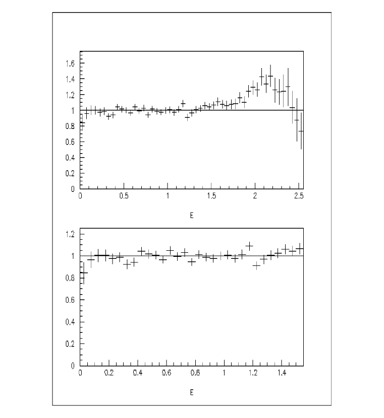
Figure 13: The ratio of the neutrino flux passing through the BooNE detector at 1000 m compared to 500 m as a function of neutrino energy in GeV. The ratio is normalized such that it equals one for a pure $1/r^{2}$ dependence. The upper figure shows the full energy range, while the lower figure enlarges the region of interest.

5.8 Beam Construction Issues

Figure 14: Southwest region of the Fermilab site. The BooNE beam line originates at MI10. Targeting and Dump Halls are located north of the MI cooling ponds. The detector is located at the northwest edge of the schematic between Giese, Kirk and Pine roads. The beam line is 1 km in length

A schematic of the site of the BooNE beam line is shown in Fig. 14. The beam line begins at MI10. The target and dump enclosures are positioned beyond the Main Injector cooling ponds. The beam direction points northwest. The detector is located 1 km from the dump enclosure.

The beam will originate at enclosure MI10. A transport pipe will be installed to bring the beam to the targeting enclosure. The length of the transport pipe will depend upon the best position of the enclosure relative to other structures, duct-work and ponds. For cost estimation purposes, we assume 100 m. Beam transport will use permanent magnets.

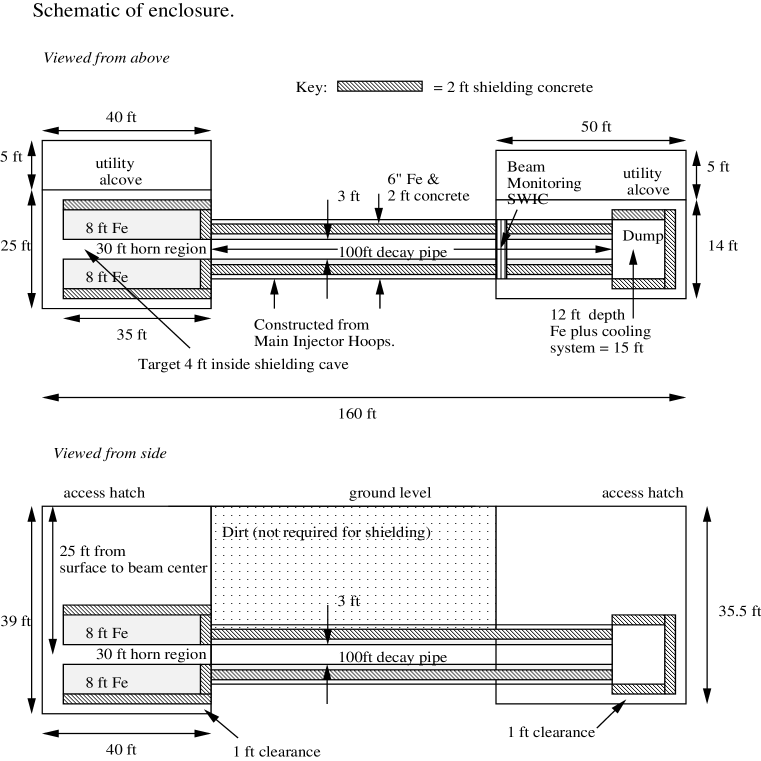
Figure 15: Schematic of enclosures with estimated shielding.

Schematics of the beam targeting enclosure, meson decay pipe and dump enclosure are shown in Fig. 15. The targeting and dump enclosures are designed to permit visual inspection of the caves, if required for radiation safety monitoring. The decay pipe will be surrounded by a structure made from Main Injector Hoops, which are 8 ft $\times$ 10 ft.

Shielding represents a significant cost because of the intensity of the beam. We have worked with Don Cossairt, Associate Head, Fermilab Radiation Protection Group, to develop a preliminary estimate for the required shielding. The shielding shown in Fig. 15 represents a conservative estimate and was determined using energy and intensity scaling of existing approved beam lines. Scaling can be used for approximating overall cost, but will not be used to determine actual shielding requirements in the final design. The CASIM program will be run during Summer, 1997, in order to accurately determine the shielding needed.

6 Detector

The MiniBooNE detector will consist of an 11.0 m diameter double-wall tank that is filled with 600 tons of mineral oil and covered on the inside with 1220 eight-inch phototubes (10% coverage). The outer volume of the tank will serve as a veto for outgoing and incoming particles.

The BooNE experiment consists of a 600 ton imaging Čerenkov detector. The detector will be placed 1000 m from the neutrino source, such that the energy distributions of $\nu_{e}C\rightarrow e^{-}X$ and $\nu_{\mu}C\rightarrow\mu^{-}X$ quasi-elastic events in the detector determine $\Delta m^{2}~{}$. Characteristics of the detector are shown in Table 4. A schematic of the proposed detector is shown in Fig. 16. The detector is a double-wall cylindrical tank, 11 m in diameter and 11 m high. The outer volume serves as a veto shield for uncontained events and is filled with a high light-output liquid scintillator. The inner (main detector) volume is a right cylinder 9.6 m in diameter and is filled with mineral oil plus a small concentration of b-PBD scintillator such that 90% of the light generated by electrons in the tank is Čerenkov light and 10% is scintillation light. A total of 1220 eight-inch photomultiplier tubes (PMTs) cover 10% of the area of the inner tank.

Figure 16: Schematic of the proposed detector.

The outer (veto) volume is equally important for identifying uncontained events and for vetoing cosmic rays. The scintillator oil in this region will be viewed by 292 PMTs distributed along the circumference of the two endcaps. The PMTs in the top ring, for example, are arranged so that half are sensitive to scintillator light from the cylindrical jacket and half to light from the top disk of veto fluid. The veto volume is separated from the main detector volume by a 2.5 cm steel wall. This wall provides optical isolation between the veto and central detector, and it helps reduce the background from $\pi^{0}~{}$ production. Neutrino induced $\pi^{0}~{}$ production is a serious background in this type of detector because of the similar behavior of gammas and electrons (see Chapter 5 for details). If only one of the gammas from a $\pi^{0}~{}$ decay converts in the main detector, that $\pi^{0}~{}$ will look like a $\nu_{e}$ appearance candidate. The 2.5 cm wall will convert about 2/3 of the escaping gammas into showers detectable by the veto shell.

In this chapter, details of the detector design are explained. Issues related to the construction are considered and the electronics and data acquisition are described. The PMTs, electronics, and data acquisition will be the same as those used for the LSND experiment.

Table 4: The characteristics of the BooNE detector.

	Detector	Veto
Volume	695 m3	400 m3
Mass	591 t	340 t
PMTs	1220(10%)	292
Fiducial Volume	449 m3
Fiducial Mass	382 t

6.1 Detector Construction Issues

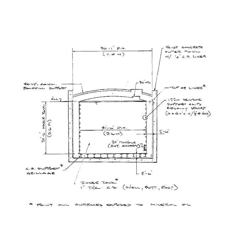
Figure 17: Schematic of the detector for cost estimates.

Several designs for the two-tank structure are under consideration, with one example shown in Figure 17. The tanks will be constructed from carbon steel. All portions of the detector exposed to oil will be painted with black epoxy. In the design shown, phototube cables exit the tanks through the manholes at the top. In the inner tank, the photoubes will be mounted on the top, bottom and walls of the tank. Each region between supporting beams at the bottom will be instrumented with multiple phototubes for vetoing cosmic rays. These phototubes are positioned by accessing the region between the tanks through the lower manhole. Veto phototubes will also be located around the circumference between the two tanks at the top facing downward. Solid scintillator will be placed across the top of the inner tank to provide the upper veto. The tanks are surrounded by a concrete structure which provides support.

The detector will be placed partially below ground level. If the above design is used, in order to provide protection from weather and dirt while phototubes are installed, an inflatable temporary dome will be placed over the top of the tank. This will be connected to a temporary portakamp where supplies can be stored. After installation of the phototubes, the inner and outer tanks will be simultaneously filled with oil. The dome and portakamp will be removed. Finally, a dirt embankment forming a hill over the tank will be installed to provide shielding for the above-ground-level portion of the detector. Electronics will be located in a trailer near to the detector.

In this letter of intent, the cost estimates for the construction of the tank system are from discussions with estimators at the Chicago Bridge and Iron Company of Plainfield, Illinois and are for the tank design shown in Fig. 17. [26]

6.2 Electronics and DAQ

The front-end electronics and the data acquisition system for BooNE must record the time of occurrence and the charge in each photomultiplier tube pulse, define a trigger for event selection, and provide for efficient event building. The system must provide time recording resolution of $\sim 0.2$ ns and charge resolution of $\sim 0.2$ pe. The system must span time scales of millisecond durations to allow for the correlations of prompt events with signals from subsequent decays. The dynamic range of the charge digitizer must be adequate to meet the needs of the event fitter and the energies that are expected from the neutrino scattering processes. Finally, the system must be low cost and fabricated with appropriate technologies. Since neutrino experiments tend to run for long periods, the system must operate reliably with low maintenance. An updated version of the LSND architecture can meet these requirements. In the following paragraphs the relevant features of the LSND electronics and data acquisition system are reviewed and the updates and modifications for the BooNE experiment are described.

The LSND data acquisition architecture consists of a fast analog front end, a flash analog to digital conversion (FADC) stage, and digital memories to store and sort the digitized data. A block diagram of this system as modified for BooNE is shown in Fig. 18. The system operates synchronously with a GPS-referenced clock providing the 100ns time base. This clock is scaled by a binary counter, the output of which is used as the address to store the digitized PMT data.

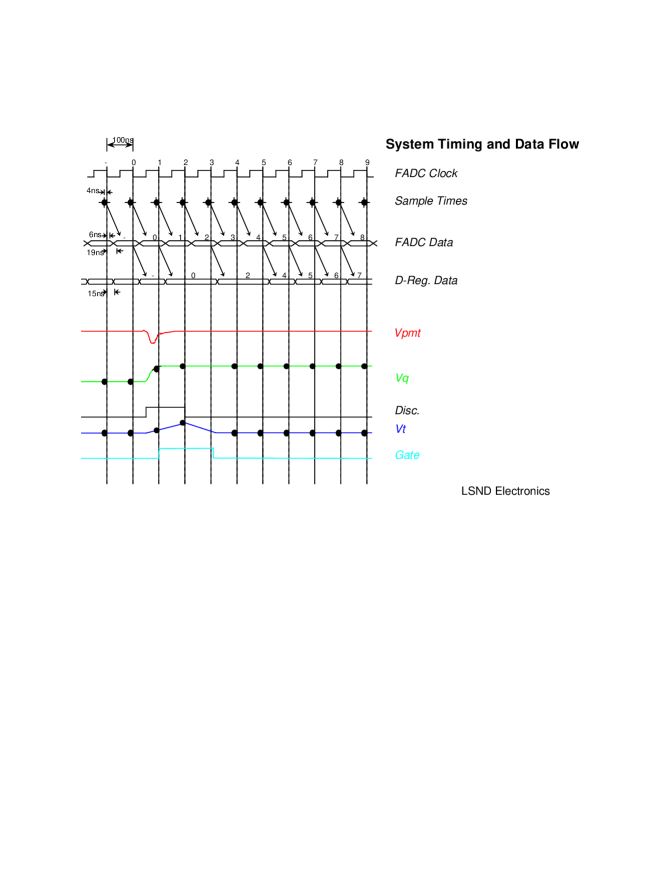
Figure 19: PMT pulse acquisition and signal timing relationships.

Each photomultiplier tube signal is connected to a channel that performs a leading edge time interval determination (the interval being between the PMT pulse and the following edge of the global clock) and an integration of the pulses. The signal acquisition and data timing are shown in Fig. 19. These signals are sampled every 100ns by FADCs and the digitized data are written into dual ported memories addressed by the global time base. At each clock tick the charge and time analog voltages are digitized by the FADCs and written into the dual ported memory. The address is then incremented and the cycle repeated. This part of the acquisition system is free running. The memories are necessarily finite in size and hold a finite time history (for LSND 204.8 $\mu$s with 100 ns resolution). They are configured as circular buffers, that is, the memory is overwritten after the clock has cycled through the address space of the memory. This provides for temporary storage of the immediate past history for a time long enough for a trigger decision to be made by a monoboard computer. It also allows for a pretrigger to determine the state of the detector prior to the arrival of an event, that is, it can “look backwards in time”.

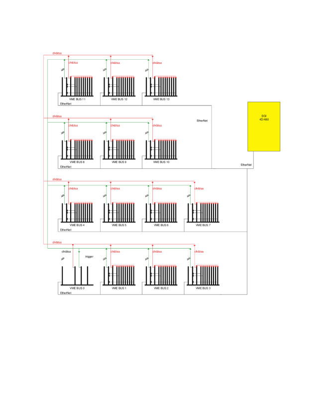
Figure 20: System configuration of the individual VME QT crates and their interconnections.

Data are extracted from the front-end dual-ported memories and built into events by the trigger system. Each front-end leading-edge discriminator provides a digital pulse to a global summation module, which computes the digital sum of all of the tubes that fired in the previous global-clock interval. A bank of digital comparators signal when the sum exceeds a preset value and the global-clock time when this happens is loaded into a FIFO memory. The trigger monoboard computer (for LSND it was an MVME-167) continually reads this FIFO. From the resulting times series of multiplicity data the trigger determines the candidate events and initiates an event build by broadcasting those global-clock times when the particular event took place to the other address port of the dual-ported memories that contain the PMT charge and time data. The system transfers the data at these “event time stamps” from their temporary location to FIFOs located adjacent to the dual-ported memories, where the data resides until read by other monoboard computers. These computers (MVME-167) calibrate and compact the data, assemble them into ethernet packets, and send them to the experiment’s analysis computer. A system configuration diagram is shown in Fig. 20.

Modifications to this system for BooNE would include the design of the appropriate trigger hardware and the modifications to the trigger acquisition code. The front-end electronics is being redesigned to make use of faster, cheaper memory to allow a larger circular buffer for a longer recorded history. A revision of the digital architecture (all components reside in VME crates) is being undertaken to simplify the dedicated data and addressing lines and keep compatibility with the VME standards. This aims to improve the reliability and reduce system costs. A new, all digital time interpolator is in design to enhance the time resolution to the 0.2 ns specification. Finally, a 10-bit or 12-bit FADC is being considered to meet the resolution-dynamic range requirements on the charge measurement. Alternatively, a dual slope analog front end is being designed that has piecewise linear gains and which matches the desired low pulse height sensitivity and large pulse height dynamic range onto the 2V range of the FADCs.

The size of each PMT window is determined by the trigger computer’s software, as is the triggering decision. It is straightforward to modify the trigger code to configure the above system for running with the beam time structure of the Fermilab booster. For example, the front-end electronics would be left free running so that the prehistory could be acquired. When the booster delivered a proton pulse to the target, a timing pulse would be generated and sent to an unused “PMT input” in the DAQ system. This would allow a precise time determination of when to begin considering events as neutrino candidates. The front end continues to record the activities in the detector, then after all anticipated events are finished, the trigger would read all of the data in the dual-ported memories. (It is more likely that such a read would begin sooner to remove any time overhead, but his is a detail in the design. The LSND system runs continuously and only reads that part of memory that contains a window 500 ns wide around a candidate event’s time stamp. The LSND system notes whether or not the accelerator has spilled beam on the neutrino production target by recording the beam status through an unused “PMT channel” as described above. Beam off events are handled identically to beam on events. The trigger does not know if the accelerator is off or on and as such is unbiased. This also allows a large sample of the background to be collected, which is of great importance for LSND. It is not as critical to the BooNE experiment, which takes place at higher energies. It may be relevant to nu-p elastic scattering, however.)

6.3 Trigger Operating Modes

The data transfer rate on the VME backplane of a QT crate is set by the monoboard computer (MBC). For LSND a Motorola MVME167 was used and had a maximum transfer rate of 20 MBytes/s, which was realized by one VME bus cycle every 200 ns. With this rate it required 13 $\mu$s to collect one time-stamp record of a full loaded QT crate, consisting of 128 PMT channels plus one header long word (260 bytes of data). To collect the six time-stamp records of an event molecule required 78 $\mu$s.

Conventional LSND DAQ operates with the trigger controlling the event builds and only selected event molecules being read from QT memory into MBC memory. In this mode the VME back plane traffic is low. In view of the (relatively) low repetition rate of the booster, several alternative modes of operation are possible. A “zero-threshold mode” that records the full detector history and a hybrid scheme that expands the history window are possible, as is a reduced threshold mode that would provide some data sparsification at the trigger level. For example, the BooNE DAQ could operate in several different scenarios:

1. LSND-mode where by an initiating “high-threshold trigger” flags a “low-threshold mode” and selected events are built. This has low back plane traffic, but at the cost of a threshold for events.

2. Zero threshold-mode where the front-end clock is enabled $\sim 50\mu$s before the proton spill begins, the time of the spill is recorded, and the clock is allowed to run for (204.8-50.0) $\mu$s before being shut off and the entire QT memory is read into MBC memory. This mode collects the entire time history of the detector from $\sim 50\mu$s prior to the spill to $\sim 150\mu$s after the spill. It requires between 13 ms to 26 ms of back plane time to read the QT memory into the MBC. Assuming a worst case of a repetition rate of 15 spills per second (66 ms per spill), this mode allows for an overhead of at least 40ms between spills for MBC processing and full event building to the main acquisition computer.

3. A hybrid scheme that takes advantage of the buffering capability of the LSND front-end memory system. This scheme leaves the front-end clock running continuously and initiates QT-memory-to-FIFO transfers $\sim 20\mu$s before the spill. This QT-memory-to-FIFO link is maintained until the FIFOs are half full, where upon the trigger interrupts this link and operates now in the LSND-low-threshold mode. The QT-FIFO readout is begun by the MBC as soon as there is data in the FIFOs, which would occur at the $\sim 20\mu$s before spill time. Notice that the data flow is event driven with throttling controls (N.B., the use of the half-full flags on the QT FIFOs) and FIFO buffer capacity to allow for smooth transfer between the no-threshold and low-threshold modes of operation.

4. A modified hybrid scheme which combines the timing with respect to the beam spill with a low threshold (but not zero) to collect events that had, e.g., greater than 4 PMTs on; rather than collect everything, which would be mostly zeros and burden the data acquisition for no good reason.

To implement these schemes on the LSND DAQ system requires the addition of a hardware card to signal the proton spill timing and the writing of new trigger software.

Figure 18: The proposed BooNE PMT channel data acquisition.

7 Detector Simulation

The GEANT-based detector Monte Carlo package accurately simulates events in the detector and allows the determination of the event reconstruction resolutions and the particle identification efficiencies. All of these techniques have been developed and tested at the LSND experiment.

7.1 GEANT Implementation

The proposed BooNE detector was simulated using the GEANT Monte Carlo package. A double wall cylindrical tank filled with mineral oil was coded into the program with dimensions as described in Section 6. An approximation of a PMT was modeled and multiple copies were positioned as shown in Fig. 16.

The GEANT implementation (V3.21) simulates the production of Čerenkov light for particles with velocities above threshold and tracks this light through the media using the (wavelength-dependent) optical properties of the mineral oil. This optical photon tracking was also used to track scintillation photons that were generated isotropically and in proportion to the amount of energy lost by charged particles in the mineral oil. These optical photons were tagged as Čerenkov or scintillation photons so that the amount of scintillation light could be adjusted in the reconstruction phase. If an optical photon intersected with the photocathode surface of the PMT volume, it was considered detected with an efficiency equal to the quantum efficiency of the PMT (also wavelength-dependent). These PMT “hits” were written to an ntuple along with the veto and input particle information.

In order to study the response of the proposed detector, first, single particle ($\mu^{\pm},e^{\pm},\pi^{0}$) events were generated isotropically over a range of energies (50-1200 MeV) within the mineral oil volume of the inner tank. Then, to better understand the relative rates for the signal and background reactions, multi-particle events of interest to the BooNE experiment were simulated. The most important reactions studied were: $\nu_{e}C\rightarrow e^{-}X$, $\nu_{\mu}C\rightarrow\mu^{-}X$, and $\nu_{\mu}C\rightarrow\nu_{\mu}\pi^{0}X$. The final states of these reactions often include an energetic proton which was included in the simulation. These events were generated within the fiducial volume of the inner tank and were weighted by the estimated cross sections and neutrino fluxes.

7.2 Event Reconstruction

Events are reconstructed using a fitting algorithm that is similar to that developed for LSND. As in LSND, the chi square of the position and angle fits ($\chi_{r}$ and $\chi_{a}$) are minimized to determine the event position and direction. In addition, these minimized chi squares, together with the fraction of PMTs with late hits ($\chi_{t}$), provide excellent particle identification and low $\mu^{\pm}-e^{\pm}$ and $\pi^{0}-e^{\pm}$ misidentification.

To determine the event position and time (corresponding to the midpoint of the track), the position chi square, $\chi_{r}$, is minimized. $\chi_{r}$ is defined as

$$\chi_{r}=\sum q_{i}\times(t_{i}-t_{o}-r_{i}/v)^{2}/Q~{},$$

where $q_{i}$ is the charge of hit phototube $i$, $t_{i}$ is the time of hit phototube i, $t_{o}$ is the fitted event time, $r_{i}$ is the distance between the fitted position and phototube i, v is the velocity of light in oil (20.4 cm/ns), $Q$ is the total number of photoelectrons in the event and the sum is over all hit phototubes. Similarly, the event direction (for particles above Čerenkov threshold) is determined by minimizing the angle chi square, $\chi_{a}$. $\chi_{a}$ is defined as

$$\chi_{a}=\sum q_{i}\times(\alpha_{i}-47^{o})^{2}/Q~{},$$

where $\alpha_{i}$ is the angle between the fitted direction and the line segment extending from the fitted position to hit phototube i, $47^{o}$ is the Čerenkov angle for $\beta\sim 1$ particles in mineral oil, and the sum is over all hit phototubes. With the track direction determined, the initial event vertex is found by using the measured track energy (which is proportional to the total number of photoelectrons in the event) to extrapolate back to the vertex.

This event reconstruction algorithm has been tested by our detector simulation discussed above. A large sample of electrons were generated uniformly in the tank and with random directions in the energy range from 50 to 1200 MeV. Fig. 21 shows the resulting position, angular, and energy resolutions. As can be seen in the figure, the position resolution is about 50 cm, the angular resolution is about $10^{o}$, and the energy resolution is about $15\%$. Note that for electrons there are about 4 photoelectrons per MeV. Furthermore, electrons can easily be distinguished from muons and neutral pions by fitting the Čerenkov ring and event vertex and by measuring the fraction of PMTs with a late hit. As seen in Fig. 22, electrons, muons, and neutral pions have quite different topologies in the tank. Fig. 23 shows $\chi_{t}$, the fraction of PMTs hit after 10 ns from the start of the event, and the $\chi_{r}$, $\chi_{a}$, $\chi_{r}\times\chi_{a}$ chi square distributions for electrons (solid curve), muons (dashed curve), and neutral pions (dotted curve) in the 50 to 1000 MeV energy range. The numbers of events are normalized and many of the muons are in the overflow bin. A clear separation is observed between electrons and muons and pions.

Figure 21: The (a) position, (b) angular, and (c) energy resolutions for a large sample of electrons generated in the tank by the detector simulation.

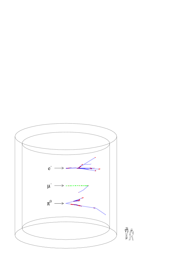
Figure 22: Typical topologies of 500 MeV electrons, muons, and neutral pions in the detector tank.

Figure 23: The (a) $\chi_{t}$, (b) $\chi_{r}$, (c) $\chi_{a}$, and (d) $\chi_{r}\times\chi_{a}$ chi square distributions for electrons (solid curve), muons (dashed curve), and neutral pions (dotted curve) in the 50 to 1000 MeV energy range. The numbers of events are normalized and many of the muons are in the overflow bin. The arrows show cuts that reduce the $\mu^{-}$ and $\pi^{0}$ by factors of 1000 and 100 relative to electrons.

8 Signal and Backgrounds for $\nu_{\mu}\rightarrow\nu_{e}$

The signature for $\nu_{\mu}\rightarrow\nu_{e}$ oscillations is $\nu_{e}$ quasi elastic scattering off carbon nuclei. The main backgrounds come from intrinsic $\nu_{e}$ contamination in the beam, mis-identified $\nu_{\mu}$ quasi elastic scattering, and neutral current $\pi^{0}$ production.

The quasi-elastic cross sections in this chapter are obtained from a modified Fermi-Gas calculation that agrees approximately with a more sophisticated continuum RPA calculation.[27] Also, the single pion cross sections are taken from Rein and Sehgal.[28]

8.1 Signal Reactions

The neutrino oscillations ($\nu_{\mu}\rightarrow\nu_{e}$ and $\bar{\nu}_{\mu}\rightarrow\bar{\nu}_{e}$) are observed by $\nu_{e}C\rightarrow e^{-}N$ and $\bar{\nu}_{e}C\rightarrow e^{+}B$ quasi elastic scattering. The cross sections for these reactions[27] are shown in Fig. 24 and Tables 5 and 6 as a function of incident neutrino energy. Note that the cross sections rise rapidly with energy near threshold and then taper off to a flat energy dependence well above threshold. Also, Fig. 25 shows the visible energy versus the neutrino energy, and Fig. 26 shows the recoil $e^{\pm}$ energy and $\cos\theta$ distributions after integrating over the incident neutrino energy spectrum. The angle $\theta$ is the reconstructed $e^{\pm}$ direction relative to the incident neutrino direction. Note that the $e^{\pm}$ has an energy on average that is about 2/3 the neutrino energy and a direction that becomes more forward peaked with energy.

Figure 24: The cross sections (in units of $10^{-38}$ cm²) for $\nu_{e}C\rightarrow e^{-}N$ and $\bar{\nu}_{e}C\rightarrow e^{+}B$ quasi elastic scattering as a function of incident neutrino energy in MeV.

Figure 25: The visible energy versus the neutrino energy in MeV from quasi elastic scattering after integrating over the incident neutrino energy spectrum.

Figure 26: The recoil $e^{\pm}$ (a) energy in MeV and (b) $\cos\theta$ distributions from quasi elastic scattering after integrating over the incident neutrino energy spectrum.

Table 5: Signal and background neutrino cross sections as a function of neutrino energy in MeV. The cross sections are for each C atom and are in units of $10^{-40}$ cm².

$E_{\nu}$(MeV)	$\nu_{e}C\rightarrow e^{-}N$	$\nu_{\mu}C\rightarrow\mu^{-}N$	$\nu_{\mu}e^{-}\rightarrow\nu_{\mu}e^{-}$	$\nu_{\mu}C\rightarrow\nu_{\mu}\pi^{0}X$	$\nu_{\mu}C\rightarrow\pi^{\pm}X$	$\nu_{\mu}C\rightarrow\mu^{-}\pi X$
100	13	0	0.01	0	0	0
200	106	63	0.03	0	0	0
300	249	213	0.04	1	0	0
400	369	341	0.05	8	1	10
500	458	435	0.06	20	8	71
600	520	501	0.08	34	17	135
700	563	546	0.09	50	24	203
800	593	575	0.10	65	32	267
900	613	596	0.11	77	39	325
1000	627	609	0.13	87	49	364
1100	636	619	0.14	92	52	394
1200	644	625	0.16	99	56	415
1300	650	629	0.17	101	57	442
1400	655	632	0.18	101	57	444
1500	659	634	0.20	102	58	450
1600	664	635	0.21	105	59	453
1700	667	636	0.22	105	59	460
1800	671	637	0.23	105	59	460
1900	675	638	0.25	105	59	460
2000	679	640	0.26	105	59	460

Table 6: Signal and background antineutrino cross sections as a function of antineutrino energy. The cross sections are for each C atom (the numbers in parentheses are the cross sections for free protons) and are in units of $10^{-40}$ cm².

$E_{\bar{\nu}}$(MeV)	$\bar{\nu}_{e}C\rightarrow e^{+}B$	$\bar{\nu}_{\mu}C\rightarrow\mu^{+}B$	$\bar{\nu}_{\mu}e^{-}\rightarrow\bar{\nu}_{\mu}e^{-}$	$\bar{\nu}_{\mu}C\rightarrow\bar{\nu}_{\mu}\pi^{0}X$	$\bar{\nu}_{\mu}C\rightarrow\pi^{\pm}X$	$\bar{\nu}_{\mu}C\rightarrow\mu^{+}\pi X$
100	7 (4)	0 (0)	0.01	0	0	0
200	32 (10)	22 (8)	0.02	0	0	0
300	59 (15)	53 (14)	0.03	1	0	0
400	84 (19)	80 (18)	0.04	5	0	4
500	109 (24)	106 (23)	0.05	11	4	31
600	133 (28)	130 (27)	0.06	18	8	59
700	156 (32)	153 (31)	0.07	26	11	89
800	176 (35)	174 (34)	0.08	34	14	117
900	195 (39)	193 (38)	0.09	40	18	142
1000	212 (42)	210 (41)	0.10	45	22	160
1100	227 (44)	226 (43)	0.11	48	23	177
1200	241 (47)	240 (46)	0.12	54	26	191
1300	253 (49)	253 (48)	0.13	56	27	213
1400	265 (51)	265 (50)	0.14	57	27	221
1500	275 (53)	275 (52)	0.15	59	29	224
1600	284 (55)	285 (54)	0.16	63	31	231
1700	292 (57)	293 (56)	0.17	65	32	246
1800	299 (58)	301 (57)	0.18	66	32	250
1900	305 (60)	307 (59)	0.19	67	33	256
2000	311 (61)	313 (60)	0.20	68	33	261

8.2 Background Reactions

A principal beam-related background is due to the intrinsic $\nu_{e}$ and $\bar{\nu}_{e}$ fluxes from kaon and muon decays discussed in chapter 5. This intrinsic background has the same reactions as the signal reactions described in section 8.1. The other main beam-related backgrounds are due to neutrino reactions that produce a $\mu^{\pm}$ or $\pi^{0}$ in the final state. The BooNE design goal is to have particle identification (PID) sufficient to suppress muon misidentification as an electron by a factor of 1000 and $\pi^{0}$ misidentification as an electron by a factor of 100. As shown in section 8.3, these suppression factors are achieved. Other backgrounds that are considered are $\pi^{\pm}$ production and $\nu e\rightarrow\nu e$ elastic scattering. A list of all of these background reactions is shown in Table 7, and the cross sections are given in Tables 5 and 6 as a function of incident neutrino energy. Note that beam-off backgrounds are expected to be very small due to the very low duty factor and can be easily subtracted by a beam-on minus beam-off subtraction.

Table 7: A list of the background neutrino reactions for $\nu_{\mu}\rightarrow\nu_{e}$ appearance. Also shown is the factor that these backgrounds can be suppressed relative to $\nu_{e}C\rightarrow e^{-}X$ scattering and the approximate background level for the appearance oscillation search.

Reaction	Suppression Factor	Background Level
$\nu_{\mu}C\rightarrow\mu^{-}X$	$10^{-3}$	$10^{-3}$
$\nu_{\mu}C\rightarrow\nu_{\mu}\pi^{0}X$	$10^{-2}$	$10^{-3}$
$\nu_{\mu}C\rightarrow\mu^{-}\pi X$	$10^{-4}$	$10^{-4}$
$\nu_{\mu}C\rightarrow\nu_{\mu}\pi^{\pm}X$	$10^{-3}$	$10^{-3}$
$\nu_{\mu}e^{-}\rightarrow\nu_{\mu}e^{-}$	$10^{-1}$	$10^{-4}$

1. $\nu_{\mu}C\rightarrow\mu^{-}N$ The first background is due to $\nu_{\mu}C\rightarrow\mu^{-}N$ and $\bar{\nu}_{\mu}C\rightarrow\mu^{+}B$ scattering, where the $\mu^{\pm}$ is misidentified as an electron. The cross sections for these reactions as a function of incident neutrino energy are shown in Fig. 27. Because these cross sections are comparable to the cross sections of the neutrino oscillation signal reactions discussed in section 7.1 above, we must be able to reject these events by a factor of $\sim 1000$ in order to achieve a neutrino oscillation sensitivity of $\sim 10^{-3}$.

Figure 27: The cross sections (in units of $10^{-38}$ cm²) for $\nu_{\mu}C$ and $\bar{\nu}_{\mu}C$ quasi elastic scattering as a function of incident neutrino energy in MeV.

2. $\nu_{\mu}C\rightarrow\nu_{\mu}\pi^{0}X$ The second background is due to $\nu_{\mu}C\rightarrow\nu_{\mu}\pi^{0}X$ and $\bar{\nu}_{\mu}C\rightarrow\bar{\nu}_{\mu}\pi^{0}X$ scattering. Fig. 28 shows the cross sections for these reactions as a function of incident neutrino energy. By comparing with the signal cross sections, it is clear that we must be able to reject these events by a factor of $\sim 100$ in order to achieve a neutrino oscillation sensitivity of $\sim 10^{-3}$.

Figure 28: The cross sections (in units of $10^{-38}$ cm²) for $\nu_{\mu}C$ and $\bar{\nu}_{\mu}C$ neutral current $\pi^{0}$ production as a function of incident neutrino energy in MeV.

3. $\nu_{\mu}C\rightarrow\nu_{\mu}\pi^{\pm}X$ The next background is due to $\nu_{\mu}C\rightarrow\nu_{\mu}\pi^{\pm}X$ and $\bar{\nu}_{\mu}C\rightarrow\bar{\nu}_{\mu}\pi^{\pm}X$ scattering. Fig. 29 shows the cross sections for these reactions as a function of incident neutrino energy. By comparing with the signal cross sections, it is clear that we must be able to reject these events by a factor of $\sim 100$ in order to achieve a neutrino oscillation sensitivity of $\sim 10^{-3}$.

Figure 29: The cross sections (in units of $10^{-38}$ cm²) for $\nu_{\mu}C$ and $\bar{\nu}_{\mu}C$ neutral current $\pi^{\pm}$ production as a function of incident neutrino energy in MeV.

4. $\nu_{\mu}C\rightarrow\mu^{-}\pi X$ Another background is due to $\nu_{\mu}C\rightarrow\mu^{-}\pi X$ and $\bar{\nu}_{\mu}C\rightarrow\mu^{+}\pi X$ scattering, where the recoil $\pi$ is a $\pi^{0}$ or $\pi^{\pm}$. Fig. 30 shows the cross sections for these reactions as a function of incident neutrino energy. By comparing with the signal cross sections, it is clear that we must be able to reject these events by a factor of $\sim 1000$ in order to achieve a neutrino oscillation sensitivity of $\sim 10^{-3}$.

Figure 30: The cross sections (in units of $10^{-38}$ cm²) for $\nu_{\mu}C$ and $\bar{\nu}_{\mu}C$ charged current pion production as a function of incident neutrino energy in MeV.

5. $\nu_{\mu}e^{-}\rightarrow\nu_{\mu}e^{-}$ The final background that we consider is $\nu_{\mu}e^{-}\rightarrow\nu_{\mu}e^{-}$ and $\bar{\nu}_{\mu}e^{-}\rightarrow\bar{\nu}_{\mu}e^{-}$ elastic scattering. The cross section for this reaction is proportional to the neutrino energy and can be expressed as $\sigma(\nu_{\mu}e^{-}\rightarrow\nu_{\mu}e^{-})=1.6\times E_{\nu}\times 10^{-42}$ cm², where the neutrino energy is in GeV. This background is small and can be identified by the recoil electron direction.

8.3 Rejection of Events with Muons and Pions

Events with a $\mu^{\pm}$, $\pi^{0}$, or $\pi^{\pm}$ in the final state are rejected by using the $\chi^{2}$ of the position fit ($\chi_{r}$) and the $\chi^{2}$ of the angle fit ($\chi_{a}$) as described in chapter 7, by vetoing events with a signal in the veto shield, and by using $\chi_{t}$, the fraction of PMTs with a late hit ($>10$ ns). By requiring, for example, $1<\chi_{a}<4$, $0<\chi_{r}<0.15$, $0<\chi_{r}\times\chi_{a}<4$, and $\chi_{t}<0.08$, we obtain a factor of $\sim 1000$ rejection of $\mu^{\pm}$ and $\pi^{\pm}$ and a factor of $\sim 100$ $\pi^{0}$ rejection relative to electrons (see Fig. 23). The $e^{\pm}$ efficiency is $\sim 50\%$. Fig. 31 shows the expected visible energy (electron equivalent) distributions from the intrinsic $\nu_{e}$ background (dashed curve), the $\nu_{\mu}C\rightarrow\mu^{-}X$ background (dotted curve), and from the $\nu_{\mu}C\rightarrow\nu_{\mu}\pi^{0}X$ background (dot-dashed curve). Also shown is the expected distribution from $\nu_{\mu}\rightarrow\nu_{e}$ oscillations for 100% transmutation. The signal to background ratio is greater than one for oscillation probabilities greater than $\sim 0.5\%$.

Figure 31: The expected visible energy (electron equivalent) distributions in MeV from the intrinsic $\nu_{e}$ background (dashed curve), the $\nu_{\mu}C\rightarrow\mu^{-}X$ background (dotted curve), and from the $\nu_{\mu}C\rightarrow\nu_{\mu}\pi^{0}X$ background (dot-dashed curve). Also shown is the expected distribution from $\nu_{\mu}\rightarrow\nu_{e}$ oscillations for 100% transmutation (solid curve).

8.4 Systematic Errors due to Background

From the present studies, 250 background events are expected in $1\times 10^{7}$ seconds of running due both to misidentification of $\mu^{\pm}$, $\pi^{0}$, or $\pi^{\pm}$ and to the intrinsic $\nu_{e}$ content of the beam. We are in the process of studying the design of our beam line and detector to improve this rate of background events. However, even with the present background expectation, a significant signal will be isolated over the full LSND region because the systematics associated with the background subtraction is expected to be less than 10%. This systematic error has been included in the sensitivities presented in this letter of intent.

For this document we have assumed a 10% error on the $\nu_{e}$ content of the beam, which is a conservative estimate based on the experience of previous analyses. Experiment 776 at Brookhaven, which used a horn focusing system, achieved a systematic error of 11% on the determination of the $\nu_{e}$ content.[29] Contributions to this uncertainty came from the $K/\pi$ ratio (10%), the $\nu_{\mu}$ statistical error (1%) and the normalization uncertainty (3%). The CCFR experiment, which used an 800 GeV proton beam to produce neutrinos and antineutrinos with a Quad Triplet system, obtained a total uncertainty in the $\nu_{e}$ content of the beam of 4.2%.[30] Noting that the kaon production from an 8 GeV beam is significantly less than for the 28 GeV proton beam at Brookhaven and using techniques developed by the CCFR and NuTeV experiment for analysis and monitoring of the flux,[31] we believe that we can obtain in the final analysis an uncertainty in the $\nu_{e}$ content of approximately 5%, but choose to use a conservative 10% error for this document.

Presently, we also assume a systematic error of 10% on the number of background events due to particle misidentification. Again, we believe that this is conservative. The Kamioka experiment, which faced similar issues of particle identification in their multi-GeV data, was able to achieve a 4% systematic error.[32] The LSND decay-in-flight analysis, which has an average neutrino energy of $\sim 150$ MeV, determines the systematic error on the muon identification to be less than 5%.[2] In MiniBooNE, the systematic error on fake quasi elastic $\nu_{e}$ events due to a misidentified muon or pion is expected to be less than 5% in the final analysis. Note that this systematic error can be determined directly from the study of events that are not misidentified and from Monte Carlo studies. Using the data to constrain the Monte Carlo in determining this background is a very powerful method which significantly reduces the error.

9 Projected Measurements and Sensitivity

The MiniBooNE experiment will be able to clearly observe neutrino oscillations in the 0.1 - 0.5 eV² mass range for values of $\sin^{2}2\theta>10^{-3}$ ($\nu_{\mu}\rightarrow\nu_{e}$ appearance) and $\sin^{2}2\theta\sim 0.5$ ($\nu_{\mu}$ disappearance).

9.1 Event Rates

For the estimation of event rates we make the following assumptions. First, we assume that the Booster operates at an energy of 8 GeV and at an average rate of 5 Hz ($2.5\times 10^{13}$ protons/s) for one year ($1\times 10^{7}$ s) at each horn-focusing polarity. Also, we assume that the fiducial volume of the detector is 382 t ($1.7\times 10^{31}$ $CH_{2}$ molecules) and that the total electron and muon efficiencies, including PID, are 50%. The resulting numbers of quasi elastic events are shown in Table 8 for both neutrino and antineutrino scattering and for the detector at a distance of 1000 m from the neutrino source. The muon-neutrino quasi elastic scattering estimates assume no oscillations, while the electron-neutrino quasi elastic scattering estimates assume 100% $\nu_{\mu}\rightarrow\nu_{e}$ transmutation.

Table 8: The estimated numbers of quasi elastic events for both neutrino and antineutrino scattering and for the detector at a distance of 1000 m from the neutrino source. The muon-neutrino quasi elastic scattering estimates assume no oscillations, while the electron-neutrino quasi elastic scattering estimates assume 100% $\nu_{\mu}\rightarrow\nu_{e}$ transmutation.

Reaction	Number of Events
$\nu_{\mu}C\rightarrow\mu^{-}X$	50,800
$\bar{\nu}_{\mu}C\rightarrow\mu^{+}X$	9,500
$\nu_{e}C\rightarrow e^{-}X$	52,500
$\bar{\nu}_{e}C\rightarrow e^{+}X$	9,600

9.2 $\nu_{\mu}\rightarrow\nu_{e}$ Appearance

Figure 32: The $\nu_{e}$ quasi elastic visible energy distribution in MeV, including oscillations and background sources, for two different possible oscillation parameters (motivated by LSND): $\Delta m^{2}=0.2$ eV² and $\sin^{2}2\theta=0.04$ (dashed) and $\Delta m^{2}=0.4$ eV² and $\sin^{2}2\theta=0.02$ (solid). Also shown in the figure is a dotted line giving the expectations for no oscillations. The two oscillation histograms include the background of the no oscillation histogram.

The detector located at 1000 m from the neutrino source will measure the $\nu_{e}$ energy spectrum through quasi elastic scattering as described in chapters 8 and 9. The event energy distribution in the detector will provide proof that neutrino oscillations are occurring and will allow the determination of the neutrino oscillation parameters (assuming that the LSND signal is indeed due to neutrino oscillations). Fig. 32 shows the $\nu_{e}$ quasi elastic event energy distribution for two different possible oscillation parameters (motivated by LSND): $\Delta m^{2}=0.2$ eV² and $\sin^{2}2\theta=0.04$ (dashed) and $\Delta m^{2}=0.4$ eV² and $\sin^{2}2\theta=0.02$ (solid). Also shown in the figure is a dotted line giving the expectations for no oscillations. Note that, as discussed in chapter 5, the neutrino flux varies as $r^{-2}$ to an excellent approximation for $r>250$ m. As is shown in the figure, neutrino oscillations can be clearly observed and measured. We estimate that, for the oscillation parameters above, $\Delta m^{2}$ can be determined with an uncertainty of $<0.2$ eV² and $\sin^{2}2\theta$ with an uncertainty of $<50\%$.

9.3 Search for CP Violation in the Lepton Sector

Assuming that $\nu_{\mu}\rightarrow\nu_{e}$ and $\bar{\nu}_{\mu}\rightarrow\bar{\nu}_{e}$ oscillations are observed, then, by comparing the neutrino and antineutrino oscillation parameters, it will be possible to make a test for CP violation in the lepton sector. CP violation may appear as a difference in the measured values of $\sin^{2}2\theta$ (or even $\Delta m^{2}$, because in general all three different $\Delta m^{2}$ values can contribute to an oscillation signal) for neutrinos compared to antineutrinos. CP violation will be observed easily if the violation is large ($>50\%$).

9.4 $\nu_{\mu}$ Disappearance

Figure 33: The $\nu_{\mu}$ quasi elastic visible energy distribution in MeV for two different possible oscillation parameters (motivated by the atmospheric neutrino problem): $\Delta m^{2}=0.2$ eV² and $\sin^{2}2\theta=0.5$ (dashed) and $\Delta m^{2}=0.4$ eV² and $\sin^{2}2\theta=0.5$ (dotted). Also shown in the figure is a solid line giving the expectations for no oscillations.

The detectors located at 1000 m from the neutrino source also will measure the $\nu_{\mu}$ energy spectrum through quasi elastic scattering as described in chapters 8 and 9. The event energy distribution can provide proof for $\nu_{\mu}$ disappearance oscillations and determine the neutrino oscillation parameters if the atmospheric neutrino problem is due to $\nu_{\mu}$ disappearance with $\Delta m^{2}>0.1$ eV². Fig. 33 shows the $\nu_{\mu}$ quasi elastic energy distribution for two different possible oscillation parameters (motivated by the atmospheric neutrino problem): $\Delta m^{2}=0.2$ eV² and $\sin^{2}2\theta=0.5$ (dashed) and $\Delta m^{2}=0.4$ eV² and $\sin^{2}2\theta=0.5$ (dotted). Also shown in the figure is a solid line giving the expectations for no oscillations. Note that, as discussed in chapter 5, the neutrino flux varies as $r^{-2}$ to an excellent approximation for $r>250$ m. As is shown in the figures, neutrino oscillations can be clearly observed and measured. We estimate that, for the oscillation parameters above, $\Delta m^{2}$ can be determined with an uncertainty of $<0.2$ eV² and $\sin^{2}2\theta$ with an uncertainty of $<50\%$.

9.5 A Method for Determining the Neutrino Flux at the Detector Location

The determination of the expected neutrino event sample has been a limitation in the systematic precision of neutrino oscillation experiments, particularly disappearance measurements. Quasi-elastic scattering off free protons has a well known cross section and can be used to reduce the systematic errors associated with scattering off neutrons and protons bound in $~{}^{12}C$. The method is described in detail elsewhere[39] and only the salient features are covered here.

There are two main points on which the method depends. First, the antineutrino cross section and its $Q^{2}$ dependence on free protons is known to about 2% in this energy and momentum transfer range, mostly because of well measured neutron decay and relatively little form factor dependence. Second, $~{}^{12}C$ is a member of a highly symmetrical isotriplet, so nuclear physics effects can be made to cancel to high accuracy. In other words, scattering from bound protons and bound neutrons are closely the same in ${}^{12}C$.

The $\bar{\nu}_{\mu}$ on $CH_{2}$ scattering events can be separated into scattering from bound and free protons using the different shapes of the respective $Q^{2}$ distributions. Since the $\bar{\nu}_{\mu}$ flux for these two samples is the same, one can then scale the bound proton cross section from the known free proton cross section. The $Q^{2}$ shape of free protons is well known,[40] and the $Q^{2}$ shape of bound protons in ${}^{12}C$ is deduced from $\nu_{\mu}$ scattering on bound neutrons. Figs. 34 and 35 show the expected $Q^{2}$ distributions for free and bound protons, using a Fermi gas model for the nuclear effects. (The Fermi gas model is just being used to indicate the expected difference in the two distributions. In the actual measurement, the $Q^{2}$ distributions will be determined from the data as discussed above.) The $\bar{\nu}_{\mu}-CH_{2}$ data is fit to the appropriate sum of the two distributions, giving the amplitudes for bound and free scattering. The amplitude of the free scattering gives an absolute value for the $\bar{\nu}_{\mu}$ flux. The amplitude of the bound scattering combined with this measured $\bar{\nu}_{\mu}$ flux gives a measurement of an effective bound proton cross section. This cross section on bound protons can then be used to infer the related effective cross section for bound neutrons.

Although there are other details discussed in reference 39, the method seems capable of yielding both neutrino and antineutrino fluxes at a level much better than previously obtained ($<15\%$). Thus, this method can be used to determine the observed flux at the detector position. A comparison of this observed flux with predictions from the beam simulation can then be interpreted in terms of neutrino oscillations.

Figure 34: The $Q^{2}$ distribution for $\bar{\nu}_{\mu}p\rightarrow\mu^{+}n$ scattering in units of MeV²/c².

Figure 35: The $Q^{2}$ distribution for $\bar{\nu}_{\mu}C\rightarrow\mu^{+}X$ scattering in units of MeV²/c², using a Fermi gas model for the nuclear effects.

9.6 An Oscillation Analysis with Reduced Systematic Errors

Another strategy for an oscillation analysis with reduced systematic errors is to divide the $\nu_{e}C\rightarrow e^{-}X$ visible energy distribution by the $\nu_{\mu}C\rightarrow\mu^{-}X$ visible energy distribution. This division removes uncertainties associated with the neutrino flux and cross sections, and, furthermore, the effect of oscillations is amplified if both $\nu_{\mu}\rightarrow\nu_{e}$ appearance and $\nu_{\mu}$ disappearance are occurring at the same $\Delta m^{2}$. Fig. 36 shows the ratio of the $\nu_{e}C\rightarrow e^{-}X$ and $\nu_{\mu}C\rightarrow\mu^{-}X$ visible energy distributions (see Figs. 32 and 33) for: (a) $\Delta m^{2}=0.2$ eV², appearance $\sin^{2}2\theta=0.04$, and disappearance $\sin^{2}2\theta=0.5$ (solid curve); (b) $\Delta m^{2}=0.4$ eV², appearance $\sin^{2}2\theta=0.02$, and disappearance $\sin^{2}2\theta=0.5$ (dashed curve); and (c) no oscillations (dotted curve). Neutrino oscillations with the above parameters can be clearly distinguished from no oscillations.

Figure 36: The ratio of the $\nu_{e}C\rightarrow e^{-}X$ and $\nu_{\mu}C\rightarrow\mu^{-}X$ visible energy distributions in MeV for: (a) $\Delta m^{2}=0.2$ eV², appearance $\sin^{2}2\theta=0.04$, and disappearance $\sin^{2}2\theta=0.5$ (solid curve); (b) $\Delta m^{2}=0.4$ eV², appearance $\sin^{2}2\theta=0.02$, and disappearance $\sin^{2}2\theta=0.5$ (dashed curve); and (c) no oscillations (dotted curve).

9.7 Non-oscillation Neutrino Physics with BooNE

With the BooNE detector and FNAL booster neutrino source, a plethora of nuclear and particle physics using the neutrino as a probe could be investigated. These topics include the role of strangeness in the proton, the behavior of the axial vector mass and coupling constant in nuclear matter, the helicity structure of the weak neutral current, and the neutrino magnetic moment. The copious flux of intermediate energy (100 MeV - 2 GeV) neutrinos from the FNAL booster source would provide a new opportunity to pursue this physics.

The list below outlines some of the interesting physics that may be investigated with BooNE. Several of the channels (namely, $\nu_{\mu}C\rightarrow\mu^{-}N$ and $\nu_{\mu}C\rightarrow\nu_{\mu}\pi^{0}X$) will need to be understood thoroughly for neutrino oscillation background estimates. The others, while not potential backgrounds, have the possibility of yielding exciting physics. More detailed feasibility studies are currently underway.

• Neutrino-Nucleon Elastic Scattering and a Measurement of $G_{s}$

  The $\nu p\rightarrow\nu p$ and $\nu n\rightarrow\nu n$ reactions (where $\nu$ is a $\nu_{\mu}$ or a $\bar{\nu}_{\mu}$) offer the possibility of extracting $G_{s}$, the strange quark axial form factor of the nucleon. The ratio of neutrino elastic scattering events producing a proton to those producing a neutron on the isoscalar carbon nucleus is a sensitive measure of $G_{s}$ and dependent only weakly upon the $F_{2}^{s}$ form factor[41]. More exactly, if this ratio is measured for both antineutrinos and neutrinos, $G_{s}$ and $F_{2}^{s}$ are separable[42]. The precision of this measurement depends upon how well the BooNE detector can distinguish neutrons from protons and is a topic that is currently under study.

• Neutrino Charged-Current Scattering

  The $\nu_{\mu}\mbox{}^{12}C\rightarrow\mu^{-}\mbox{}^{12}N$ and $\bar{\nu}_{\mu}\mbox{}^{12}C\rightarrow\mu^{+}\mbox{}^{12}B$ reactions will be measured to high precision with BooNE. By comparing the two as a function of $Q^{2}$, which allows a separation of the free protons from the bound protons in the $\bar{\nu}_{\mu}$ channel (see section 9.5), $M_{A}$, the axial-vector dipole mass, in the nuclear medium will be measured.

• Neutral-Current $\pi^{0}$ Production

  A measure of $\nu_{\mu}C\rightarrow\nu_{\mu}\pi^{0}X$ is a sensitive probe of the structure of the weak neutral-current. Significant gains in precision will be achieved over previous experiments in this energy region. This will enable a test of the standard model prediction of the helicity structure of the weak neutral-current.

• Neutrino-Electron Neutral-Current Scattering

  By measuring the $\nu_{\mu}e^{-}\rightarrow\nu_{\mu}e^{-}$ cross section and its behavior at low-$Q^{2}$, evidence for (or a limit on) a magnetic moment of the muon-neutrino will be obtained. If the neutrino is a Majorana particle (and CPT holds) the neutrino must have no magnetic moment. Thus, a measurement of a non-vanishing magnetic moment is proof that the neutrino is a Dirac particle. This is also relevant to the solar neutrino problem.

10 BooNE: A Future Upgrade to Two Detectors

Given an oscillation signal in the MiniBooNE experiment, a second detector will be added to determine the oscillation parameters. This also permits a sensitive search for CP violation in the lepton sector.

Given that an oscillation signal is observed in MiniBooNE, then the next goals would be:

• to determine the oscillation parameters from both $\nu_{\mu}\rightarrow\nu_{e}$ and $\nu_{\mu}$ disappearance.

• to search for CP violation in the Lepton Sector.

A natural upgrade to the MiniBooNE experiment that addresses these goals is to add a second detector. The energy dependence of the ratio of neutrino events in the two detectors determines the oscillation parameters. Comparison of results from running in neutrino mode to antineutrino mode investigates CP violation. A summary of the expectations of this two-detector experiment is provided here.

The second detector will be a double-wall cylindrical tank of the same design as the MiniBooNE detector. The outer volume serves as a veto shield for uncontained events and is filled with high light-output liquid scintillator. The inner (main detector) volume is a right cylinder, 9.6 m in height and 9.6 m in diameter, that is filled with mineral oil. The inner detector has 1220 eight-inch photomultiplier tubes of the type used for the MILAGRO experiment (Hammamatsu R5912). The electronics and data acquisition would be similar to the LSND design. The tank would be placed partially underground, with overburden to reduce the rate of cosmic ray muons and eliminate the cosmic ray hadronic component. An approximate cost estimate for this detector is given in Table 14.

The new, near detector will be placed approximately 500 meters from the neutrino source. The MiniBooNE detector would be used as the far detector, located at 1000 meters from the beam line target. These distances are chosen to provide the optimum comparison between the rate of events in the near and far detector, as discussed below. The MiniBooNE beam line will be used to provide the neutrino and antineutrino beams for both detectors.

10.1 Event Rates for BooNE

Table 9: The estimated numbers of quasi elastic events for both neutrino and antineutrino scattering and for both the near (500 m) and far (1000 m) detectors. The muon-neutrino quasi elastic scattering estimates assume no oscillations, while the electron-neutrino quasi elastic scattering estimates assume 100% $\nu_{\mu}\rightarrow\nu_{e}$ transmutation.

Reaction	Near Detector	Far Detector
$\nu_{\mu}C\rightarrow\mu^{-}X$	609,600	152,400
$\bar{\nu}_{\mu}C\rightarrow\mu^{+}X$	114,000	28,500
$\nu_{e}C\rightarrow e^{-}X$	630,000	157,500
$\bar{\nu}_{e}C\rightarrow e^{+}X$	115,200	28,800

For the estimation of event rates we make the following assumptions. First, we assume that the Booster operates at an energy of 8 GeV and at an average rate of 5 Hz ($2.5\times 10^{13}$ protons/s) for 3 years of operation ($3\times 10^{7}$ s) at each focusing polarity. Also, we assume that the fiducial volume of the detector is 382 t ($1.7\times 10^{31}$ $CH_{2}$ molecules) and that the total electron and muon efficiencies, including PID, are 50%. The resulting numbers of quasi elastic events are shown in Table 9 for both neutrino and antineutrino scattering and for both the near (500 m) and far (1000 m) detectors. The muon-neutrino quasi elastic scattering estimates assume no oscillations, while the electron-neutrino quasi elastic scattering estimates assume 100% $\nu_{\mu}\rightarrow\nu_{e}$ transmutation.

10.2 $\nu_{\mu}\rightarrow\nu_{e}$ Appearance

The two detectors located at 500 m and 1000 m from the neutrino source will measure the $\nu_{e}$ energy spectrum through quasi elastic scattering as described in chapters 8 and 9. The energy-dependent ratio of event rates from the two detectors will provide proof that neutrino oscillations are occurring and will allow the determination of the neutrino oscillation parameters (assuming that the LSND signal is indeed due to neutrino oscillations). Fig. 37 shows the ratio of $\nu_{e}$ quasi elastic events from the detectors at 500 m and 1000 m as a function of visible energy for four different possible oscillation parameters (motivated by LSND): (a) $\Delta m^{2}=0.2$ eV² and $\sin^{2}2\theta=0.04$; (b) $\Delta m^{2}=0.4$ eV² and $\sin^{2}2\theta=0.02$; (c) $\Delta m^{2}=0.6$ eV² and $\sin^{2}2\theta=0.01$; (d) $\Delta m^{2}=0.8$ eV² and $\sin^{2}2\theta=0.008$. For each set of oscillation parameters it is conservatively assumed that the total background rate from all sources (intrinsic $\nu_{e}$ component in the beam, $\pi^{0}$ background, $\mu$ background, etc.) is 0.5% of the $\nu_{\mu}\rightarrow\nu_{e}$ 100% transmutation rate. Also shown in the figures (at a ratio of 1) are solid lines giving the expectations for no oscillations. Note that, as discussed in chapter 5, the neutrino flux varies as $r^{-2}$ to an excellent approximation for $r>250$ m. As is shown in the figures, neutrino oscillations can be clearly observed and measured. We estimate that, for the oscillation parameters above, $\Delta m^{2}$ can be determined with an uncertainty of $<0.1$ eV² and $\sin^{2}2\theta$ with an uncertainty of $<25\%$.

Figure 37: The ratio of $\nu_{e}$ quasi elastic events from the detectors at 500 m and 1000 m as a function of visible energy in MeV for four different possible oscillation parameters (motivated by LSND): (a) $\Delta m^{2}=0.2$ eV² and $\sin^{2}2\theta=0.04$; (b) $\Delta m^{2}=0.4$ eV² and $\sin^{2}2\theta=0.02$; (c) $\Delta m^{2}=0.6$ eV² and $\sin^{2}2\theta=0.01$; (d) $\Delta m^{2}=0.8$ eV² and $\sin^{2}2\theta=0.008$. Also shown in the figures (at a ratio of 1) are solid lines giving the expectations for no oscillations.

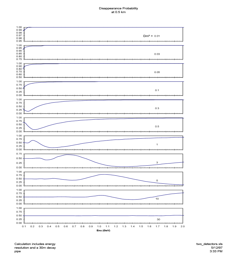
Figure 38: The dependence on energy of events at the near (500 m) detector for full mixing and various $\Delta m^{2}$ values.

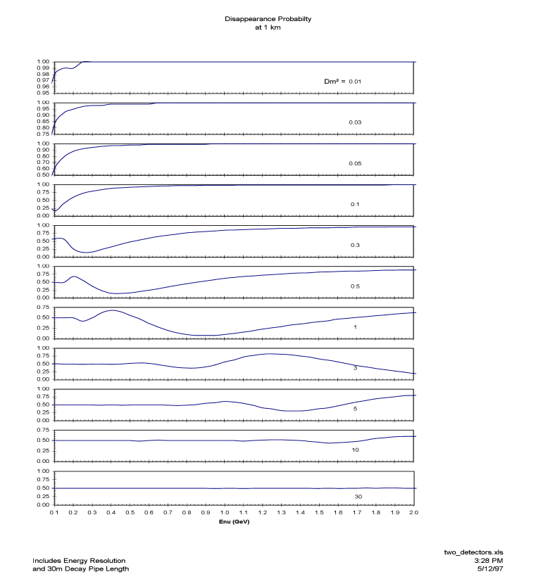
Figure 39: The dependence on energy of events at the far (1000 m) detector for full mixing and various $\Delta m^{2}$ values.

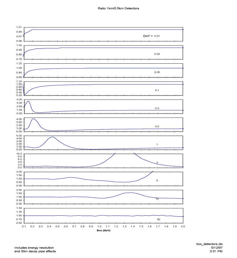
Figure 40: The ratio of events at the near (500 m) and far (1000 m) detectors as a function of energy for full mixing and various $\Delta m^{2}$ values.

Figure 41: The ratio of $\nu_{\mu}$ quasi elastic events from the detectors at 1000 m and 500 m as a function of visible energy in MeV for three different possible oscillation parameters (motivated by the atmospheric neutrino problem): (a) $\Delta m^{2}=0.1$ eV² and $\sin^{2}2\theta=0.5$; (b) $\Delta m^{2}=0.2$ eV² and $\sin^{2}2\theta=0.5$; (c) $\Delta m^{2}=0.4$ eV² and $\sin^{2}2\theta=0.5$. Also shown in the figures (at a ratio of 1) are solid lines giving the expectations for no oscillations.

10.3 $\nu_{\mu}$ Disappearance

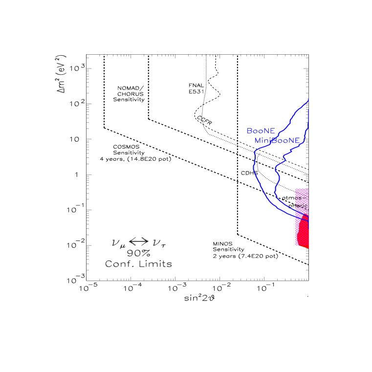
Figure 42: Summary of results from past experiments (narrow, dashed and dotted), future approved experiments (wide, dashed) and 90% C.L. limit expected for the two-detector configuration, BooNE, (solid) for $\nu_{\mu}$ disappearance after one year of running at 1 km. Solid region indicates the favored region for the atmospheric neutrino deficit from the Kamioka experiment. A result from Kamiokanda indicating no zenith angle dependence extends the favored region to higher $\Delta m^{2}$ as indicated by the hatched region.

The two detectors located at 500 m and 1000 m from the neutrino source also will measure the $\nu_{\mu}$ energy spectrum through quasi elastic scattering as described in chapters 8 and 9. The energy-dependent ratio of event rates from the two detectors can be used to observe $\nu_{\mu}$ disappearance oscillations and determine the neutrino oscillation parameters. Figures 38 and 39 shows how the visible energy will change with $\Delta m^{2}$ for full mixing for the 500 m and 1000 m detectors, respectively. Figure 40, shows the ratio for full mixing. Motivated by the atmospheric neutrino problem, Fig. 41 shows the ratio of $\nu_{\mu}$ quasi elastic events from the detectors at 1000 m and 500 m as a function of visible energy for: (a) $\Delta m^{2}=0.1$ eV² and $\sin^{2}2\theta=0.5$; (b) $\Delta m^{2}=0.2$ eV² and $\sin^{2}2\theta=0.5$; (c) $\Delta m^{2}=0.4$ eV² and $\sin^{2}2\theta=0.5$. Also shown in these figures (at a ratio of 1) are solid lines giving the expectations for no oscillations. Note that, as discussed in chapter 5, the neutrino flux varies as $r^{-2}$ to an excellent approximation for $r>250$ m. As is shown in the figures, neutrino oscillations can be clearly observed and measured. We estimate that, for the oscillation parameters above, $\Delta m^{2}$ can be determined with an uncertainty of $<0.1$ eV² and $\sin^{2}2\theta$ with an uncertainty of $<25\%$. The expected limits if no signal is observed is shown in Fig. 42.

10.4 Search for CP Violation in the Lepton Sector

Assuming that $\nu_{\mu}\rightarrow\nu_{e}$ and $\bar{\nu}_{\mu}\rightarrow\bar{\nu}_{e}$ oscillations are observed, then, by comparing the neutrino and antineutrino oscillation parameters, it will be possible to make a test for CP violation in the lepton sector. CP violation may appear as a difference in the measured values of $\sin^{2}2\theta$ (or even $\Delta m^{2}$, because in general all three different $\Delta m^{2}$ values can contribute to an oscillation signal) for neutrinos compared to antineutrinos. We estimate that CP violation can be observed easily if the violation is large ($>25\%$).

11 Cost and Schedule

The cost of the MiniBooNE detector and neutrino beam line are estimated to be $1.6M and $3M, respectively. A reasonable time scale is the commencement of data taking in 2001.

Table 10: Existing materials for the MiniBooNE Experiment. a) Materials committed by Los Alamos National Laboratory and universities. b) Request to Fermilab for use of materials existing on site.

A. Materials to be provided by LANL and universities for Detector
Item	Source	Value in thousands
1512 Phototubes	LANL	$1210
Cabling and connectors	LANL	$50
Channel Electronics	LANL	$422
Electronics Hut	LANL	$100
Remote DAQ	LANL	$250
Dilute Scintillator Oil	LANL	$185
Scintillator Oil	LANL	$110
Solid Scintillator	Univ, LANL	$400
Phototubes for solid scintillator	Univ	$25
Total value of goods:		$2535
B. Materials requested from Fermilab
Item	Present Location	Value in thousands
Liquid Scintillator (5500 gallons)	NuTeV Detector	$56
Iron (2200 ft3)	NuTeV Detector	$110
Solid Scintillator	NuTeV Detector	$100
Beam Monitors & Electronics	NuTeV Beam Line	$100
Portakamp	Not yet identified	$100
Total value of goods:		$366

This chapter outlines the costs of MiniBooNE. The detector and the beam line are considered separately. The cost of a second detector for the Phase II upgrade is also presented. The costs described here include equipment and construction.

The cost of engineering is not included. LANL is prepared to provide some engineering, with $100K in funds earmarked for engineering design of the MiniBooNE detector in fiscal year 1998.

The cost of MiniBooNE is held to a modest level by re-using equipment. Table 10a lists the materials which will be contributed by LANL and the universities on the experiment. The total of equipment which is already committed to the project, mainly by LANL, is over $2.5 million, where the listed value is based on the present purchase cost of similar equipment.

Fermilab has solicited requests to reuse equipment from detectors which are to be dismantled.[43] Table 10b lists existing materials at Fermilab which we are specifically requesting. We request to be notified if any further liquid scintillator or solid scintillator becomes available from Fermilab experiments which will be dismantled. The portakamp will be for temporary use during the construction phase in order to maintain a clean entrance to the detector and provide space for testing equipment. Thus the portakamp will become available to the lab again after 2000. We plan to make use of some NIM electronics from PREP which is presently in use within the NuTeV trigger system. We request that all of the NuTeV trigger system NIM logic be reassigned to MiniBooNE. We request that the lemo cables and terminators from NuTeV be reserved for MiniBooNE.

Table 11: Cost Estimate for the 8 GeV proton-generated neutrino beam.

Item	Cost in thousands
Permanent Quadrupole Magnets (@ $2K per 20 m)	$10
Permanent Dipole Magnet (@ $10K per magnet)	$10
Vacuum system (@ $300K per km)	$30
Focusing apparatus	$100
Rapid cycling power supply for focusing	$200
Beam monitoring equipment	$50
Total of beam line elements	$400
Shielding surrounding target and decay pipe	$300
Dump, including cooling and shielding	$150
Total for shielding and dumps	$450
Conventional construction	$ 2000
Utilities	$ 150
Total enclosure costs	$2150
Total without contingency	$3000

A cost estimate for the beam is summarized in Table 11. The cost of the beam line is mainly due to the enclosures which must be centered 25 ft below surface level. The low energy neutrino beam, which is used for both phases of the experiment, is of conventional design and therefore of relatively low cost. The 8 GeV transport system using permanent magnets is particularly economical. The cost of the focusing apparatus is estimated by the cost of a Lithium Lens. Note that the rapid cycling power supply for the focusing system appears as a separate item. Beam monitoring equipment from the NuTeV experiment is expected to be re-used, so only $50K is assigned to this item.

Table 12: Unit cost of the 0.6 kton MiniBooNE detector with mineral oil. Costs reflect the the fact that some material are already available to members of the BooNE Collaboration.

Item	Cost in thousands
Two-tank system	$350
Tank installation (Conventional construction)	$300
Temporary inflatable domed roof	$25
Phototubes	$0
Phototube Mounts	$15
Mineral Oil	$555
Veto Scintillator Oil	$236+$0
Veto Solid Scintillator	$0
Cabling and connectors	$0
Channel Electronics	$0
Electronics Hut	$0
Remote DAQ	$0
Liquid Handling	$50
Other Shipments	$50
Support Utilities	$50
Total without contingency	$1631

Approximate costs for the MiniBooNE detector are listed in Table 12. These represent the actual expected expenditures rather than the net worth of the equipment. Therefore, the cost has been adjusted for materials which are already owned or are available to members of the MiniBooNE collaboration. The cost of the tank system and construction comes from discussions with the Chicago Bridge and Iron Company or Plainfield Illinois. These represent only cost estimates.[26] We assume that the detector will contain a dilute scintillator mixture formed by combining the LSND scintillator (1/4 of the total volume) with mineral oil. Computing for analysis will be supplied by LANL and the universities.

Table 13: Milestones for MiniBooNE

1997	Finalize Design
	Complete Approvals Process
1998	Detector engineering complete
	Engineering of rapid-cycling power supply
	Engineering of the beam line enclosures
1999	Tank installation
	Construction of the beam line enclosures
	Construction of horn and power supply system
	Engineering of the remaining beam line elements
	Recommissioning/ building of beam line monitors
2000	Electronics and Phototube installation
	Installation of the beam line elements
2001	Begin taking data

Once funding has been secured, it is estimated that the detector construction will take two years. A reasonable time scale has construction starting in 1999 and the commencement of data taking in 2001. Table 13 describes the milestones in the process of commissioning MiniBooNE. A substantial amount of work is already scheduled for the summer, including: finalizing the horn design (G. Mills, H. White), addressing whether the detector should contain dilute mineral oil (W. Louis), writing the triggering software for MiniBooNE (R. Tayloe, D. Matzner), testing phototubes (T. Ochs, B. Tamminga), completing CASIM studies (J. Conrad, M. Petravick), and other projects. The expectation is that a formal proposal will be provided to the PAC in the autumn.

As discussed in chapter 10, a second detector is needed if a signal is observed in MiniBooNE in order to accurately measure the mixing and mass parameters. The costs associated with this second detector, assuming that it is identical in design to the MiniBooNE detector, are listed in table  14. Located at 500m from the beam dump, this detector will be centered 12ft below ground level. Thus the cost of the conventional construction is higher than for MiniBooNE. The MiniBooNE domed roof will be re-used.

Table 14: Unit cost of a second 0.6 kton second detector with mineral oil for Phase II (BooNE).

Item	Cost in thousands
Two-tank system	$450
Tank installation (Conventional construction)	$600
Temporary inflatable domed roof	$0
Phototubes	$1210
Phototube Mounts	$15
Dilute Scintillator	$740
Veto Scintillator Oil	$402
Veto Solid Scintillator	$280
Cabling and connectors	$50
Channel Electronics	$422
Electronics Hut	$100
Remote DAQ	$250
Liquid Handling	$50
Support Utilities	$100
Total without contingency	$4669

12 Conclusions

The MiniBooNE experiment will have the capability of observing both $\nu_{\mu}\rightarrow\nu_{e}$ appearance and $\nu_{\mu}$ disappearance. It will also search for CP violation in the lepton sector.

We propose to construct and operate a neutrino detector system and broad band neutrino beam generated from the Fermilab Booster that has the capability of observing and measuring $\nu_{\mu}\rightarrow\nu_{e}$ oscillations and $\nu_{\mu}$ disappearance over a wide range of $\Delta m^{2}$. The motivation for this experiment stems from the LSND neutrino oscillation result[1] and the atmospheric neutrino problem. The relatively low energy (0.1 - 2.0 GeV) neutrino beam combined with a detector distance of 1km will cover the interesting $\Delta m^{2}$ region between $0.01$ and $1.0$ eV² for modest cost and effort. The proposed MiniBooNE experiment would start with a single detector with the goal of probing this mass region and establishing definitive indications of neutrino oscillations. If a positive signal is observed, a second stage, BooNE, would use two detectors in the same neutrino beam to accurately determine the oscillation parameters and investigate any CP violating $\nu_{\mu}/\bar{\nu}_{\mu}$ effects.

The MiniBooNE experiment will use one detector at a distance of 1 km from the neutrino beam source. The high intensity available from the Booster combined with an efficient horn-focused secondary beam will provide over 50,000 events per year in the 400 ton detector. With this setup, the intrinsic $\nu_{e}$ component of the beam is less than $3\times 10^{-3}$ due to the little kaon production by 8 GeV primary protons and reduced muon decay in the short 30 m decay pipe. The totally active MiniBooNE detector also has good particle identification capabilities and the expected mis-identification fraction is at the $2\times 10^{-3}$ level. Comparisons of the observed $\nu_{e}$ and $\nu_{\mu}$ energy distributions with expectations will allow a sensitive search for $\nu_{\mu}\rightarrow\nu_{e}$ oscillations and $\nu_{\mu}$ disappearance.

If oscillations exist at the LSND level, MiniBooNE should see several hundred anomalous $\nu_{e}$ events over background and establish the signal at the $>5\;\sigma$ level. From the energy dependence of the excess, the oscillation parameters can be determined in the LSND region with a $\Delta m^{2}$ $(\sin^{2}2\theta)$ uncertainty of $<0.2$ eV² ($<50\%$) respectively. Examining the signal with both incident $\nu_{\mu}$ and $\bar{\nu}_{\mu}$ will allow a first look at possible CP violation effects in the lepton mixing matrix. On the other hand, if no oscillation signal is observed, the experiment will significantly extend the region probed for oscillations and exclude $\nu_{\mu}\rightarrow\nu_{e}$ oscillations with $\sin^{2}2\theta>6\times 10^{-4}$ for large $\Delta m^{2}$ and $\Delta m^{2}>0.01$ eV² for $\sin^{2}2\theta=1$.

In summary, the MiniBooNE experiment will make a sensitive search for $\nu_{e}$ appearance and $\nu_{\mu}$ disappearance from neutrino oscillations in the $\Delta m^{2}$ region between 0.01 and 1 eV². The experiment has unique capabilities and sensitivity to measure oscillations in this region in a cost effective and timely manner.

References

References

- [1] C. Athanassopoulos et. al. , Phys. Rev. Lett. 75, 2650 (1995); C. Athanassopoulos et. al. , Phys. Rev. Lett. 77, 3082 (1996); C. Athanassopoulos et. al. , Phys. Rev. C. 54, 2685 (1996).
- [2] C. Athanassopoulos et. al. , submitted to Phys. Rev. C.
- [3] C. Cardall and G. M. Fuller, Phys. Rev. D 53, 3532(1996); G. L. Fogli, E. Lisi, and G. Scioscia, hep-ph/9702298.
- [4] K. Eitel, “Recent results and upgrade from KARMEN,” Presented at Workshop on Fixed Target Physics at the Main Injector, May, 1997, and private communications.
- [5] K. S. Hirata et. al. , Phys. Lett. B280, 146 (1992).
- [6] R. Becker-Szendy et. al. , Phys. Rev. D46, 3720 (1992).
- [7] Y. Hirata et. al. , Phys. Lett. B335, 237 (1994).
- [8] R. Clark et. al. , submitted to Phys. Rev. Lett.
- [9] R. Davis, Prog. Part. Nucl. Phys. 32, 13 (1994).
- [10] J. N. Abdurashitov et. al. , Phys. Lett. B 328, 234 (1994); P. Anselmanni et. al. , Phys. Lett. B 328, 377 (1994).
- [11] Y. Fukuda et. al. , Phys. Lett. B 335, 237 (1994).
- [12] N. Hata and P. Langacker, Phys. Rev. D 50, 632(1994);
- [13] J. N. Bahcall and M. M. Pinsonneault, Rev. Mod. Phys. 64, 885 (1992).
- [14] T. Gaisser and M. Goodman, Proceedings of the 1994 Snowmass Summer Study, Particle and Nuclear Astrophysics in the Next Millenium; E. W. Kolb R. D. Peccei eds, World Scientific 1994
- [15] T. K. Gaisser and J. S. O’Connell, Phys. Rev. D 34, 822 (1986); W. M. McDonald, E. T. Dressler and J. S. O’Connell, Phys. Rev. C 19, 455 (1979). The 12C nucleus is modeled with binding energy 25 MeV, Fermi momentum 220 MeV/c, and six neutrons.
- [16] P.F. Harrison, D.H. Perkins, and W.G Scott, Phys. Lett. B349 (1995) 137 and e-Print Archive: hep-ph/9702243, submitted to Phys. Lett. B.
- [17] L. A. Ahrens et. al. , Phys. Rev. D 34, 75 (1986).
- [18] B. Bodmann et. al. , Phys. Lett. B 267, 321 (1991); B. Bodmann et. al. , Phys. Lett. B 280, 198 (1992); B. Zeitnitz et. al. , Prog. Part. Nucl. Phys., 32 351 (1994).
- [19] L. Borodovsky et. al. , Phys. Rev. Lett. 68, 274 (1992).
- [20] B. Achkar et. al. , Nucl. Phys. B434, 503 (1995).
- [21] F. Dydak et. al. , Phys. Lett. B 134, 281 (1984).
- [22] C. Athanassopoulos et. al. , Phys. Rev. Lett. 75, 2650 (1995).
- [23] R. Becker-Szendy et. al. , Phys. Rev. D46, 3720 (1992).
- [24] M. C. Goodman, Nucl. Phys. B (Proc. Suppl.) 38, 337 (1995).
- [25] The Beamline Monitoring section was contributed by R. Drucker, University of Oregon, Beamline Monitoring Expert for NuTeV.
- [26] N. Bacon, Business Development Manager, Chicago Bridge and Iron Company, Private Communication, April 28, 1997; Subsequent discussions on April 30, 1997.
- [27] E. Kolbe, K. Langanke, and S. Krewald, Phys. Rev. C 49, 1122 (1994); (K. Langanke, private communication).
- [28] D. Rein and L. M. Sehgal, Ann. of Phys. 133, 79 (1981); D. Rein and L. M. Sehgal, Nucl. Phys. B223, 29 (1983).
- [29] L. Borodovsky, thesis, Columbia University, Nevis-275 (1991).
- [30] B. King, thesis, Columbia University, Nevis-283 (1994).
- [31] Bernstein,et al., FNAL TM-1884 (1995).
- [32] K. Nishikawa, Proc. WIN95, Talloires, France, 300 (1995).
- [33] K. Eitel, thesis, Universitat und Forschungszeutrum Karlsruhe (1995); Forschungszeutrum Karlsruhe report FZKA 5684 (1995).
- [34] L. A. Ahrens et. al. , Phys. Rev. D 31, 2732 (1985).
- [35] K. S. McFarland et. al. , Phys. Rev. Lett. 75, 3993 (1995); C. Haber et. al. , Phys. Rev. Lett. 52, 1384 (1984).
- [36] G. Zacek et. al. , Phys. Rev. D 34, 2621 (1986).
- [37] G. S. Vidyakin et. al. , JETP Letters 59, 364 (1984).
- [38] N. Ushida et. al. , Phys. Rev. Lett. 57, 2897 (1986).
- [39] D. H. White, LSND TN-114 (1997).
- [40] C. H. Llewellyn Smith, Physics Reports 3, 262 (1972); P. Vogel, Phys. Rev. D 29, 1918 (1984); E. J. Beise and R. D. McKeown, Comm. Nucl. Part. Phys. 20, 105 (1991).
- [41] G. Garvey, E. Kolbe, K. Langanke, and S. Krewald, Phys. Lett. B 289, 249 (1992).
- [42] G. Garvey, E. Kolbe, K. Langanke, and S. Krewald, Phys. Rev. C 48, 1919 (1993).
- [43] “Reuse of Equipment,” Fermilab Workshop on Fixed Target Physics at the Main Injector, May, 1997.