AMD + HF model and its application to Be isotopes

In order to study light unstable nuclei systematically, we propose a new method ”AMD + Hartree-Fock”. This method introduces the concept of the single particle orbits into the usual AMD. Applying AMD + HF to Be isotopes, it is found that the calculated lowest intrinsic states with plus and minus parities have rather good correspondence with the explanation by the two-center shell model. In addition, by active use of the single particle orbits extracted from AMD wave function, we construct the first excited 0⁺ state of ¹⁰Be. The obtained state appears in the vicinity of the lowest 1^- state. This result is consistent with the experimental data.

I Introduction

For the study of the structure of light unstable nuclei which are and have been extensively studied experimentally by the use of radioactive beams [1-3], various theories [4-20] have been used [21,22] . Among those theories, the antisymmetrized molecular dynamics (AMD) approach has already proved to be useful and successful[23]. One of the large merits of the AMD approach is that it does not rely on any model assumptions such as axial symmetry of the deformation, existence of the clustering and so on.

Until now this AMD approach has not explicitly utilized the concept of the single particle motion in the mean field. The experimental data, however, show that very often we can get better understanding of the structure of unstable nuclei in terms of the single particle motion in the mean field. In order to see this point in more detail, we here discuss briefly some features of Be isotopes as an example. In Be isotopes there is the famous problem that the ground state ¹¹Be has an anomalous parity. According to the usual shell model, its spin-parity should be $\frac{1}{2}^{-}$. But in experiments it is $\frac{1}{2}^{+}$. An answer to this problem is that due to the deformation the $\Omega^{\pi}$=$\frac{1}{2}^{+}$ level in sd shell comes down below the upper $\Omega^{\pi}$=$\frac{1}{2}^{-}$ and the last neutron occupies the lowered $\Omega^{\pi}$=$\frac{1}{2}^{+}$. ¹¹Be is also famous as a halo nucleus. Since the lowered orbit contains s-orbit component, we can understand that the halo property is due to the long tail of the s-orbit. For the convenience of later discussion we call this lowered $\Omega^{\pi}$=$\frac{1}{2}^{+}$ level ” halo level”.

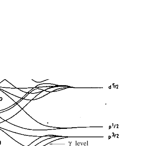
FIG. 1.: The complete neutron level scheme of the two-center shell model as a function of the eccentricity parameter $Z_{0}$. On the ordinate at the left are given the spherical shell model states of the original nucleus together with the energy scale, while on the right-hand side the quantum numbers of the spherical shell model states in the fragment nuclei are seen. This figure is quoted from [24].

In order to discuss other Be isotopes than ¹¹Be, we use the single particle diagram by the two-center shell model[18-20], which is shown in FIG.1[24]. According to the AMD calculation for Be isotopes, we can support the idea that Be isotopes have the core part with an approximate dumbbell structure of two $\alpha$ clusters, which is the reason why we use the two-center shell model. ⁹Be is known to have three rotational bands which have the band head states with J^π=$\frac{3}{2}^{-}$, $\frac{1}{2}^{-}$ and $\frac{1}{2}^{+}$. We can explain these three bands in the two-center shell model as follows. We put the four neutrons in order from the lowest level at about Z₀=2.5 fm in this model, and when the last neutron is put in the levels of $\Omega^{\pi}$=$\frac{3}{2}^{-}$($\alpha$ level), $\frac{1}{2}^{-}$($\beta$ level) and $\frac{1}{2}^{+}$($\gamma$ level) , J^π becomes $\frac{3}{2}^{-}$, $\frac{1}{2}^{-}$ and $\frac{1}{2}^{+}$, respectively. Here, Z₀ is the eccentricity parameter, namely the distance between two centers in FIG.1. ¹⁰Be is known to have two rotational bands which have the band head states with J^π=0⁺ and 1^-. In the same way as above, the four neutrons are put in order from the lowest level at about Z₀=3 fm and when the configurations of the last two neutrons are $[\Omega^{\pi}=\frac{3}{2}^{-}]^{2}$ and $[\Omega^{\pi}=\frac{3}{2}^{-}]^{1}[\Omega^{\pi}=\frac{1}{2}^{+}]^{1}$, J^π becomes 0⁺ and 1^-, respectively. Here we note that the $\Omega^{\pi}$= $\frac{1}{2}^{+}$ level is the halo level which appeared in ¹¹Be.

These arguments show that by using the single particle orbits and by constructing the excited state by particle-hole excitation we can study the structure of Be isotopes systematically. Therefore we recognize the importance of the single particle motion in the mean field.

In this paper we propose the ”AMD + Hartree-Fock” method (AMD+HF) which introduces the concept of the single particle orbits into the usual AMD. We extract the component of the mean field from the AMD wave function. Once we get the single particle wave functions in the mean field, we can study the structure of the excited states by constructing various particle-hole configurations. When we need elaborate description of the single particle motion like in the case of neutron halo phenomena, we need to improve the AMD single particle wave function in such a way that we adopt the superposition of several Gaussians instead of the single Gaussian wave packet in the usual AMD.

This paper is composed of six sections. In the second section we explain the formalism of AMD+HF method. In the third section we show the single particle levels of the ground states of Be isotopes which are calculated with AMD+HF. In the forth section we show the single particle levels obtained with AMD+HF as a function of the deformation parameter. In the fifth section, based on the motivation of the AMD+HF, which means active use of the single particle levels, we construct the first plus-parity excited state of ¹⁰Be by putting two neutrons into the halo level and study it. And the last section is for the discussion and the summary.

II AMD+HF method

A Variation under the constraint of deformation

1 Hamiltonian and wave function

In this paper, we used the Hamiltonian and wave function as described below.

The Hamiltonian has the form:

$$\hat{H} = \hat{T}+\hat{V}_{c}+\hat{V}_{LS}-\hat{T}_{G}.$$

Here $\hat{T}$, $\hat{V}_{c}$, $\hat{V}_{LS}$ and $\hat{T}_{G}$ stand for the kinetic energy, the central force, the LS force and the center-of-mass kinetic energy, respectively. We neglected the Coulomb force. we used the Volkov No.1 force[25] as the central force and the G3RS force[26] for the LS force. These forces have the following forms,

$$\hat{V}_{c} = \frac{1}{2}\sum_{i,j}(w+b\hat{P}_{\sigma}+h\hat{P}_{\tau}-m\hat{P}_{\sigma}\hat{P}_{\tau})[V_{R}e^{-({\hat{\bf r}}_{ij}/r_{R})^{2}}+V_{A}e^{-({\hat{\bf r}}_{ij}/r_{A})^{2}}],$$

$$\hat{V}_{LS} = \frac{1}{2}\sum_{i,j}V_{LS}[e^{-({\hat{\bf r}}_{ij}/r_{LSR})^{2}}-e^{-({\hat{\bf r}}_{ij}/r_{LSA})^{2}}]P(^{3}O)\hat{\bf L}_{ij}(\hat{\bf s}_{i}+\hat{\bf s}_{j}),$$

where m=0.56, w=1$-$m, b=h=0, V_R=144.86 MeV, V_A=$-$83.34 MeV, r_R=0.82 fm, r_A=1.6 fm, V_LS=900 MeV, r_LSR=0.20 fm, r_LSA=0.36 fm. P(³O) is the projection operator onto the triplet odd state.

The wave function of total system is expressed by a Slater determinant:

$$|\Phi> = \det[|\varphi_{i}(j)>],$$

$$<{\bf r}|\varphi_{i}> = (\frac{2\nu}{\pi})^{3/4}\sum_{\alpha}C_{i}^{\alpha}\exp[-\nu({\bf r}-\frac{{\bf Z}_{i}^{\alpha}}{\sqrt{\nu}})^{2}\;|\beta_{i}>,$$

where $|\beta_{i}>$ is the spin-isospin function. In AMD+HF, single particle wave function is in general a linear combination of several Gaussians in order to describe single particle state more adequately than usual AMD. However in this paper we represented the single particle state by a single Gaussian wave packet for simplicity. $|\Phi>$ is projected to parity eigenstates $|\Phi^{\pm}>$ and the energy variation is made after parity projection.

$$|\Phi^{\pm}> = \frac{1}{\sqrt{2}}[|\Phi>\pm{\cal P}|\Phi>].$$

2 Cooling equation with constraint

As mentioned above, the wave function is parameterized by $\{C^{\alpha}_{i},{\bf Z}^{\alpha}_{i}\}$. These parameters are determined by solving the following cooling equation,

$$\dot{X}_{i} = (\lambda+i\mu)\frac{1}{i\hbar}\frac{\partial{\cal H}}{\partial X_{i}^{*}}\hskip 14.22636pt{\rm and}\hskip 8.5359ptC.C.,$$

$${\cal H} = \frac{<\Phi^{\pm}|\hat{H}|\Phi^{\pm}>}{<\Phi^{\pm}|\Phi^{\pm}>}.$$

Here $\{X_{i}\}$ means $\{C^{\alpha}_{i},{\bf Z}^{\alpha}_{i}\}$, $\lambda$ is an arbitrary real number and $\mu$ is a negative arbitrary number. We can easily prove that the energy of the total system decreases with time,

$$\frac{d}{dt}{\cal H} < 0.$$

We often need to obtain the minimum-energy state under some condition. For example, the condition is that the center-of-mass is fixed to the coordinate origin, or that the deformation parameter is fixed to some value, etc. In such case, the condition is combined to the cooling equation by the analogy of the Lagrange-multiplier method. When the condition is represented as ${\cal W}$(X${}_{i}^{\alpha}$,X${}_{i}^{\alpha*}$)=0, the previous cooling equation is changed as below:

$$\dot{X}_{i} = (\lambda+i\mu)\frac{1}{i\hbar}[\frac{\partial{\cal H}}{\partial X_{\imath}^{*}}+\eta\frac{\partial{\cal W}}{\partial X_{\imath}^{*}}]\hskip 14.22636pt{\rm and}\hskip 8.5359ptC.C.,$$ (1)

where $\eta$ is a Lagrange-multiplier function, which is determined by $\frac{d}{dt}{\cal W}=0$:

$$0 = \frac{d}{dt}{\cal W}$$

$$= \sum_{i}[\frac{\partial{\cal W}}{\partial X_{\imath}}\dot{X}_{i}+\frac{\partial{\cal W}}{\partial X_{\imath}^{*}}\dot{X}_{i}^{*}]$$

$$= \sum_{i}[\frac{\partial{\cal W}}{\partial X_{\imath}}\{(\lambda+i\mu)\frac{1}{i\hbar}(\frac{\partial{\cal H}}{\partial X_{\imath}^{*}}+\eta\frac{\partial{\cal W}}{\partial X_{\imath}^{*}})\}$$

$$\mbox{}+\frac{\partial{\cal W}}{\partial X_{\imath}^{*}}\{(\lambda-i\mu)\frac{-1}{i\hbar}(\frac{\partial{\cal H}}{\partial X_{\imath}}+\eta\frac{\partial{\cal W}}{\partial X_{\imath}})\}].$$

From this equation we get

$$\eta = -\frac{\cal F}{\cal G},$$

$${\cal F} = \sum_{i}[(1-i\frac{\lambda}{\mu})\frac{\partial{\cal W}}{\partial X_{\imath}}\frac{\partial{\cal H}}{\partial X_{\imath}^{*}}+(1+i\frac{\lambda}{\mu})\frac{\partial{\cal W}}{\partial X_{\imath}^{*}}\frac{\partial{\cal H}}{\partial X_{\imath}}],$$

$${\cal G} = 2\sum_{i}\frac{\partial{\cal W}}{\partial X_{\imath}}\frac{\partial{\cal W}}{\partial X_{\imath}^{*}}.$$

One may think that this method is applied only to the case where the number of conditions is one. But we can use it also in the case where several conditions exist. When several conditions are represented as

$${\cal W}_{1}=0,{\cal W}_{2}=0,\cdots,{\cal W}_{n}=0,$$

these conditions can be represented by a single equation,

$${\cal W}=c_{1}|{\cal W}_{1}|^{2}+\cdots+c_{n}|{\cal W}_{n}|^{2}=0.$$

Here $c_{1}\cdots c_{n}$ are positive coefficients which adjust the difference of scale between ${\cal W}_{1},{\cal W}_{2},\cdots,{\cal W}_{n}$. By this way, we can always use Eq.(1) without introducing several Lagrange-multipliers.

3 Deformation parameter

The deformation parameter ($\beta$,$\gamma$) can be obtained from the following relations,

$$A_{x}\equiv\frac{<x^{2}>^{\frac{1}{2}}}{[<x^{2}><y^{2}><z^{2}>]^{\frac{1}{6}}} = \exp[\sqrt{\frac{5}{4\pi}}\beta\cos(\gamma+\frac{2\pi}{3})],$$

$$A_{y}\equiv\frac{<y^{2}>^{\frac{1}{2}}}{[<x^{2}><y^{2}><z^{2}>]^{\frac{1}{6}}} = \exp[\sqrt{\frac{5}{4\pi}}\beta\cos(\gamma-\frac{2\pi}{3})],$$

$$A_{z}\equiv\frac{<z^{2}>^{\frac{1}{2}}}{[<x^{2}><y^{2}><z^{2}>]^{\frac{1}{6}}} = \exp[\sqrt{\frac{5}{4\pi}}\beta\cos\gamma],$$

where

$$<x^{2}> = \frac{<\Phi|\frac{1}{A}\sum_{i}x_{i}^{2}|\Phi>}{<\Phi|\Phi>},\hskip 14.22636pt{\rm etc.}$$

Here x, y, z directions are the directions of the principal axes of inertia which are the coordinate axes of the body-fixed frame. We can easily confirm that this definition of deformation parameter is the same as that of Bohr model to the first order. Here expectation value of every operator is calculated with the intrinsic wave function before parity projection. In addition $<x^{2}>$, $<y^{2}>$ and $<z^{2}>$ is redefined so that $<z^{2}>\geq<y^{2}>\geq<x^{2}>$. We must note the fact that in this definition z axis is not always the axial symmetric axis of the system. In the case of prolate deformation, z axis determined by this definition is certainly the axial symmetric axis, while in the case of oblate deformation it is not the axial symmetric axis.

When we execute the cooling calculation with deformation constraint, it consumes time that in every step of the cooling we calculate the inertial axes to determine the deformation parameters. Therefore we use rotational invariant scalar quantities for calculating the deformation parameters so as to avoid the time-consuming procedure. We define the tensor quantity Q in any coordinate system as below:

$$Q_{ij} = <r_{i}r_{j}>,$$

where i, j are x, y, z. Then calculating the trace of the tensors Q and QQ, we get the rotational invariant quantities TrQ and TrQQ. Since calculating these quantities in the space-fixed frame is identical to that in body-fixed frame, we obtain the following relations:

$$TrQ_{space-fixed} = TrQ_{body-fixed}$$

$$= \sum_{i}<r^{2}_{i}>_{body-fixed}=[<x^{2}><y^{2}><z^{2}>]^{\frac{1}{3}}\sum_{i}A_{i}^{2}$$

$$= [<x^{2}><y^{2}><z^{2}>]^{\frac{1}{3}}\cdot(3+\frac{15}{4\pi}\beta^{2}+\cdots),$$

$$TrQQ_{space-fixed} = TrQQ_{body-fixed}$$

$$= \sum_{i}<r^{2}_{i}>^{2}_{body-fixed}=[<x^{2}><y^{2}><z^{2}>]^{\frac{2}{3}}\sum_{i}A_{i}^{4}$$

$$= [<x^{2}><y^{2}><z^{2}>]^{\frac{2}{3}}\cdot(3+\frac{15}{\pi}\beta^{2}+\cdots).$$

Using these quantities, we define D as below:

$$D \equiv \frac{TrQQ}{(TrQ)^{2}}\hskip 28.45274pt{\rm in}\hskip 5.69046pt{\rm space-fixed\;frame}.$$

Then we can calculate the deformation parameter $\beta$ as

$$\beta \simeq \sqrt{\frac{2\pi}{5}(3D-1)}.$$

Thus we can obtain $\beta$ without using the inertial axes. This approximation is enough correct to the second order of $\beta$, which in ordinary case is less than unity.

When we impose the constraint that $\beta$ is fixed to some $\beta_{0}$, we use D and D₀ corresponding to $\beta$ and $\beta_{0}$ in the cooling calculation. The constraint condition function ${\cal W}_{D}$ is given as

$${\cal W}_{D} = (D-D_{0})^{2}.$$

B Single particle orbits described by AMD

1 Method of calculating single particle orbits

As mentioned in the introduction, we need to calculate the single particle orbits. We calculate them by the method shown below. This method extracts the single particle orbits from AMD wave function by mimicking the Hartree-Fock theory.

In the Hartree-Fock method, the matrix elements h_ij of the single particle Hamiltonian in orthonormal base $\{|\phi_{i}>\}$ are given as

$$h_{ij} = <\phi_{i}|\hat{t}|\phi_{j}>+\sum_{k}<\phi_{i}\phi_{k}|\hat{v}(|\phi_{j}\phi_{k}>-|\phi_{k}\phi_{j}>).$$

By diagonalizing this h_ij, we obtain the set of the single particle wave functions and the single particle energies. Now we construct Hartree-Fock-like single particle orbits and levels from total wave function of AMD. The single particle wave functions $\{\varphi_{i}\}$ of AMD are not orthonormal. So first we construct the orthonormal base by making linear-combination of $\{\varphi_{i}\}$. We calculate the set of eigenvalues and eigenvectors of the overlap matrix B,

$$\sum_{j}B_{ij}c^{\alpha}_{j} = \mu^{\alpha}c^{\alpha}_{i},$$

$$B_{ij} \equiv <\varphi_{i}|\varphi_{j}>.$$

Eigenvectors $\{c^{\alpha}_{i}\}$ are normalized. We define new base $\{|f^{\alpha}>\}$ as follows:

$$|f_{\alpha}> = \frac{1}{\sqrt{\mu^{\alpha}}}\sum_{i}c^{\alpha}_{i}|\varphi_{i}>.$$

We can confirm easily that this set forms an orthonormal base.

Using this base $|f^{\alpha}>$ we construct the matrix $\{h_{\alpha\beta}\}$ corresponding to the single particle Hamiltonian of Hartree-Fock as follows:

$$h_{\alpha\beta} = <f_{\alpha}|\hat{t}|f_{\beta}>+\sum_{\gamma}<f_{\alpha}f_{\gamma}|\hat{v}(|f_{\beta}f_{\gamma}>-|f_{\gamma}f_{\beta}>).$$

Diagonalizing this matrix $\{h_{\alpha\beta}\}$, we calculate the eigenvalues $\{\epsilon^{p}\}$, and eigenvectors $\{g^{p}_{\alpha}\}$,

$$\sum_{\beta}h_{\alpha\beta}g^{p}_{\beta} = \epsilon^{p}g^{p}_{\alpha}.$$

The eigenvectors $\{g^{p}_{\alpha}\}$ are normalized. The single particle wave function $|p>$ belonging to the single particle energy $\epsilon^{p}$ is given as

$$|p> = \sum_{\alpha}g_{\alpha}^{p}|f^{\alpha}>$$

$$= \sum_{\alpha}g_{\alpha}^{p}[\frac{1}{\sqrt{\mu^{\alpha}}}\sum_{i}c^{\alpha}_{i}|\varphi_{i}>]$$

$$= \sum_{i}[\sum_{\alpha}g_{\alpha}^{p}\frac{1}{\sqrt{\mu^{\alpha}}}c^{\alpha}_{i}]|\varphi_{i}>.$$

We call such single particle orbits $\{|p>\}$ and energies $\{\epsilon^{p}\}$ AMD-HF orbits and energies, respectively since they are extracted from AMD wave function.

Here we should note that these orbits and energies of AMD-HF are not totally equivalent to those of Hartree-Fock. The reason is as below. In AMD+HF, the Hartree-Fock equation is solved only within the functional space of single particle wave functions which is spanned by $\{\varphi_{i}\}$. Thus in AMD+HF the Hartree-Fock self-consistency is satisfied only within this restricted functional space. We can regard the AMD+HF method as being a kind of restricted Hartree-Fock method. However this restriction has a large merit because the functional space spanned by the single particle wave functions $\{\varphi_{i}\}$ is obtained by the energy variation including parity projection.

2 Identification of AMD-HF orbits

We need to identify the AMD-HF orbits $|p>$ defined in the previous section. As almost nuclei seem to have axially symmetric deformation approximately, we expect that z component of the total angular momentum, $\hat{j}_{z}$, is approximately a good-quantum number, but that the magnitude of it, $\hat{\bf j}^{2}$, is not. In addition, when the states that have the same absolute value of $j_{z}$ are degenerate, the expectation value of $\hat{j}_{z}$ doesn’t give us useful information. Therefore we use the square of $\hat{j}_{z}$ ,$\hat{j}_{z}^{2}$, so as to avoid this difficulty. For example, let us consider the state $|p>$ which includes $|j_{z}=m>$ and $|j_{z}=-m>$ as below:

$$|p> = \frac{1}{\sqrt{1+|c|^{2}}}\;[\;|m>+c|-m>].$$

The expectation value of $\hat{j}_{z}$ is

$$<p|\hat{j}_{z}|p> = m\cdot\frac{1-|c|^{2}}{1+|c|^{2}}.$$

On the other hand, the expectation value of $\hat{j}_{z}^{2}$ is

$$<p|\hat{j}_{z}^{2}|p> = m^{2},$$

from which we can identify m certainly.

By the way, this identification is done on the body-fixed frame as noticed in the section about calculating the deformation. Here we calculate the inertial axes explicitly by diagonalizing the tensor $Q_{ij}$, which was introduced in section II.A.3. We choose the z-axis of the body-fixed frame to the direction of the $Q^{space}$’s eigenvector which has the largest eigenvalue. Here $Q^{space}$ represents Q calculated in the space-fixed frame. Using the eigenvector ${\bf c}^{q}$, we can relate $\hat{\bf j}^{space}$ and $\hat{\bf j}^{body}$ as follows:

$$\hat{j}^{body}_{q} = {\bf c}^{q}\cdot\hat{\bf j}^{space},$$

where $\hat{\bf j}^{space}$ and $\hat{\bf j}^{body}$ are the total angular momentum operator in space-fixed frame and that in the body-fixed frame, respectively. Thus the square $j_{z}$ in the body-fixed frame is represented using the quantities in the space-fixed frame as below:

$$<p|\hat{j}^{2}_{z}|p>_{body-fixed} = \sum_{ij}c^{z}_{i}c^{z}_{j}<p|\hat{j}_{i}\hat{j}_{j}|p>_{space-fixed}.$$

In addition, we use also the square of the orbital angular momentum $\hat{\bf l}^{2}$, which is not a good-quantum number. This enables us to relate the obtained levels to the levels which would be obtained if the shape were spherical.

III AMD-HF orbits in Be isotopes

In this section we show the results about AMD-HF orbits of the ground states that are obtained by AMD. Here AMD single particle wave functions are composed of the single Gaussians.

In TABLE I, the AMD-HF levels are given. $\Omega^{2}$ and $L^{2}$ indicate the expectation values of the operators $\hat{j}_{z}^{2}$ and $\hat{\bf l}^{2}$ respectively, which are obtained by the method mentioned in section II.B.2. $\beta$ and B.E. are the deformation parameter and the binding energy respectively. We explain the results, about ⁹Be, ¹⁰Be and ¹¹Be, that look interesting. Then we compare these with the simple model — two-center shell model — to help our understanding.

a.⁹Be

In the minus-parity AMD state of ⁹Be, $\Omega^{2}$ of the highest level of neutron is 1.260, which is not equal to any of 0.25(=$(\frac{1}{2})^{2}$), 2.25(=$(\frac{3}{2})^{2}$), etc. This means the deformation is not axial symmetric. But $L^{2}$=2.995 implies that this level contains rather large amount of the 0p${}_{\frac{3}{2}}$ component.

In the plus-parity state, the last neutron is in the level of $\Omega=\frac{1}{2}$. In addition $L^{2}$ of this level is 4.884. As this value is rather large, we can suppose that this level consists largely of d-orbit. In the two center shell model given in FIG.1, the plus-parity level named $\gamma$ level in FIG.1 comes down in energy when the distance between two alpha clusters is large. This is consistent with our result because the deformation parameter $\beta$ obtained in AMD for the plus-parity state is 0.801, which is very large.

6Be(+)   B.E.=-21.26 MeV   $\beta$=0.437
s.p. energy	$\Omega^{2}$	${\bf l}^{2}$	occ.	plus
proton
$-$2.48	0.250	2.077	2	7.4
$-$24.47	0.250	0.118	2	96.0
neutron
$-$29.51	0.250	0.148	2	93.1
7Be($-$)   B.E.=$-$30.48 MeV   $\beta$=0.566
s.p. energy	$\Omega^{2}$	${\bf l}^{2}$	occ.	plus
proton
$-$11.04	0.250	2.083	2	5.1
$-$28.88	0.250	0.219	2	96.5
neutron
$-$11.15	0.250	2.059	1	4.3
$-$28.87	0.250	0.224	1	96.5
$-$32.04	0.250	0.440	1	82.2
8Be(+)   B.E.=$-$48.00 MeV   $\beta$=0.656
s.p. energy	$\Omega^{2}$	${\bf l}^{2}$	occ.	plus
proton
$-$18.99	0.250	2.189	1	2.3
$-$19.58	0.250	2.127	1	0.2
$-$34.69	0.250	0.345	2	100.0
neutron
$-$18.87	0.250	2.203	1	2.7
$-$19.55	0.250	2.131	1	0.3
$-$34.69	0.250	0.345	2	99.7
9Be($-$)   B.E.=$-$46.96 MeV   $\beta$=0.521
s.p. energy	$\Omega^{2}$	${\bf l}^{2}$	occ.	plus
proton
$-$21.82	0.249	2.098	2	0.7
$-$39.03	0.250	0.231	2	99.7
neutron
+1.56	1.260	2.996	1	21.8
$-$18.18	0.269	2.147	1	2.8
$-$21.82	0.249	2.098	1	0.7
$-$33.70	0.256	0.297	1	99.1
$-$39.03	0.249	0.230	1	99.7
9Be(+)   B.E.=$-$42.97 MeV   $\beta$=0.801
s.p. energy	$\Omega^{2}$	${\bf l}^{2}$	occ.	plus
proton
$-$22.48	0.250	2.287	2	3.1
$-$35.04	0.250	0.494	2	99.6
neutron
+6.79	0.250	4.885	1	79.8
$-$18.07	0.250	2.280	1	4.5
$-$22.37	0.250	2.320	1	4.1
$-$31.45	0.250	0.483	1	98.6
$-$35.06	0.250	0.475	1	99.4

10Be(+)   B.E.=$-$53.11 MeV   $\beta$=0.381
s.p. energy	$\Omega^{2}$	${\bf l}^{2}$	occ.	plus
proton
$-$23.00	0.254	2.049	2	0.5
$-$43.30	0.254	0.108	2	99.6
neutron
$-$7.47	1.241	2.487	2	12.7
$-$19.55	0.278	2.162	2	3.2
$-$37.72	0.257	0.100	2	99.7
10Be($-$)   B.E.=$-$44.95 MeV   $\beta$=0.637
s.p. energy	$\Omega^{2}$	${\bf l}^{2}$	occ.	plus
proton
$-$24.65	0.250	2.106	2	0.0
$-$39.75	0.250	0.304	2	100.0
neutron
$-$3.41	0.667	3.387	2	59.4
$-$20.39	0.264	2.328	2	1.4
$-$35.23	0.254	0.270	2	99.7
11Be(+)   B.E.=$-$47.25 MeV   $\beta$=0.505
s.p. energy	$\Omega^{2}$	${\bf l}^{2}$	occ.	plus
proton
$-$25.97	0.250	2.089	2	1.9
$-$44.97	0.250	0.140	2	99.4
neutron
+4.25	0.272	4.463	1	97.1
$-$6.74	1.273	2.153	1	3.7
$-$8.84	1.253	2.543	1	12.3
$-$17.75	0.250	2.327	1	2.5
$-$22.47	0.258	2.264	1	6.2
$-$35.43	0.252	0.147	1	99.8
$-$39.55	0.255	0.134	1	99.8
11Be($-$)   B.E.=$-$54.70 MeV   $\beta$=0.271
s.p. energy	$\Omega^{2}$	${\bf l}^{2}$	occ.	plus
proton
$-$24.97	0.250	2.034	2	1.2
$-$48.62	0.250	0.042	2	99.7
neutron
$-$2.52	1.314	2.350	1	8.2
$-$7.15	1.241	2.315	1	7.5
$-$10.75	1.388	2.311	1	7.4
$-$18.04	0.251	2.144	1	4.7
$-$21.55	0.259	2.115	1	2.9
$-$36.61	0.250	0.051	1	99.7
$-$42.60	0.253	0.035	1	100.0

TABLE I. Single particle levels of the ground state of each nucleus. ”B.E.” and ”$\beta$” are the binding energy and the deformation parameter, respectively. ”occ.” indicates the occupation number of the level. ”plus” indicates the percentage of plus-parity component. We regard two levels as the same level whose energy difference is less than 100 keV. In such case, the difference in $\Omega^{2}$ and ${\bf l}^{2}$ is about 0.01.

b.¹⁰Be

The calculated plus-parity state of ¹⁰Be has a good correspondence with the two-center shell model, if we think our highest level of neutron corresponds to the level named the $\alpha$ level in FIG.1 which comes from $j_{z}$=$\frac{3}{2}$ of 0p${}_{\frac{3}{2}}$ in spherical case.

But on the other hand, the minus-parity state does not have a similarity with the two-center shell model. The most surprising point is that the only three spectra of neutron appeared in our calculation. In the two-center shell model every single particle level is the eigenstate of parity. So in the model four spectra should appear. The explanation of this result by AMD+HF is as below: “ The single particle orbit (AMD-HF orbit) extracted from AMD wave function is the parity-mixing state. And the last two neutrons are degenerate in that state.” Explaining this phenomenon in terms of the two-center shell model is as follows. At some distance between two $\alpha$ particles, the levels $\Omega=\frac{3}{2}$ and $\Omega=\frac{1}{2}$, coming from 0p${}_{\frac{3}{2}}$ and 0d${}_{\frac{5}{2}}$ respectively, approach each other. As a result, these levels are mixed, and then we see the only one level in which two levels are mixed. Here we investigate the percentage of parity-mixing in the last AMD-HF orbit of neutron. This AMD-HF level, which is represented as $|f>$, can be written as follows:

$$|f> = \epsilon_{1}|+>+\epsilon_{2}|->,$$

$$\epsilon_{1}^{2}+\epsilon_{2}^{2}=1,$$

where $|+>$ and $|->$ indicate plus- and minus-parity components, respectively. Using the operator ${\cal P}$ which reverses the parity, we calculate the following quantity A:

$$A \equiv <f|{\cal P}|f>=\epsilon_{1}^{2}-\epsilon_{2}^{2}.$$

Then we obtain the ratio as follows:

$$\epsilon_{1}^{2}=\frac{1+A}{2}\;,\;\epsilon_{2}^{2}=\frac{1-A}{2}.$$

Calculated results are $\epsilon_{1}^{2}$=0.60 and $\epsilon_{2}^{2}$=0.40. As we expected this level is a state with large parity-mixing.

c.¹¹Be

In the calculated plus-parity state of ¹¹Be, the last neutron occupies what we call ”halo level”. $\Omega^{2}$=0.25 means $\Omega$=$\frac{1}{2}$ and $L^{2}$=4.463 of this level means that this level contains a large component of 0d${}_{\frac{5}{2}}$. We think that this result is similar to that of the two-center shell model with medium distance between two $\alpha$ particles. The obtained value of the deformation parameter $\beta$=0.504, which is medium, is consistent with the medium distance in the two-center shell model.

However in the calculated minus-parity state of ¹¹Be, we don’t find so good similarity between AMD+HF and the two-center shell model. As $\beta$=0.271 is rather small, we try to compare the obtained result to that of the two-center shell model with small inter-$\alpha$ distance. In that case, the last neutron should be put into the level named the $\beta$ level in FIG.1 which has $\Omega$=$\frac{1}{2}$ and comes from 0p${}_{\frac{1}{2}}$ in spherical case. But according to AMD+HF calculation, $\Omega^{2}$ of the last neutron level is 1.314, which means that $\Omega$ is not $\frac{1}{2}$.

By the way, there is the famous problem in ¹¹Be, which is that the parity of the ground state is not minus but plus. In this calculation, we have not succeeded to reproduce this anomalous parity just like the previous AMD calculation of Ref.[23]. We think that this failure comes from the insufficient description of the single particle orbits in the present calculation where we have assigned only one Gaussian for one nucleon.

IV AMD-HF orbits with constrained deformation

In this section, we show the AMD-HF orbits at various $\beta$, which look like Nilsson diagram. The levels at each $\beta$ are calculated by the method as mentioned in the section II.A.2. As in the previous section, we show only the results about ⁹Be($-$), ¹⁰Be($-$) and ¹¹Be($-$), which look interesting. We show the diagram of the neutron’s AMD-HF levels of ⁹Be($-$), ¹⁰Be($-$) and ¹¹Be($-$) in FIG.2(a), FIG.3(a) and FIG.4(a), respectively. As the behavior of the highest level in each diagram looks especially interesting, we show the variation of $L^{2}$, $\Omega^{2}$ and the percentage of the plus-parity component of the highest level in FIG.2(b), FIG.3(b) and FIG.4(b). In addition as the second and the third levels in ¹¹Be($-$) look interesting too, we show the same quantities about these levels in FIG.4(c) and FIG.4(d). Notice that the scale on the right hand side is used for the percentage of the plus-parity component.

a.⁹Be($-$)

FIG. 2.: (a) Diagram of the AMD-HF levels of ⁹Be($-$). (b) Variation of $L^{2}$, $\Omega^{2}$ and the percentage of the plus-parity component of the highest level.

In FIG.2(a) we can see the inversion or the crossing of the single particle levels like that appearing in the two-center shell model. When we trace the behavior of the last neutron’s level, in FIG.2(b) we see that up to $\beta$=0.67 the last level seems to be $|\Omega|=\frac{3}{2}$ coming from 0p${}_{\frac{3}{2}}$ in spherical case. But beyond $\beta$=0.67, its behavior changes apparently. Suddenly $L^{2}$ becomes rather large, $\Omega^{2}$ becomes about 0.25 and the percentage of the plus-parity component becomes about 100%. Therefore we can recognize it as the lowered halo level that is $|\Omega|=\frac{1}{2}$ coming from 0d${}_{\frac{5}{2}}$. We notice that the behaviors of the other levels than the highest level are also changed beyond $\beta$=0.67 in FIG.2(a), but that $L^{2}$,$\Omega^{2}$ and the percentage of the plus-parity component are not changed. As the parity of the last neutron is almost plus beyond $\beta$=0.67, the total intrinsic wave function is an almost plus-parity state. Therefore the projection to the minus-parity state is made by picking up the very small component of minus parity.

b.¹⁰Be($-$)

In FIG.3(a), we can see that the last neutron’s level keeps to be parity-mixed even if $\beta$ is changed. When we look at the behavior of the quantum numbers $\Omega$ and L in FIG.3(b), we find that as $\beta$ becomes larger $|\Omega|$ approaches to $\frac{1}{2}$ and L increases too. This result seems to indicate that this level has two components, one being $|\Omega|=\frac{1}{2}$ coming from 0d${}_{\frac{5}{2}}$ and the other being $|\Omega|=\frac{3}{2}$ coming from 0p${}_{\frac{3}{2}}$, and that as $\beta$ becomes larger the component of $|\Omega|=\frac{1}{2}$ increases. In addition, according to the parity-mixing ratio, this insight seems to be correct, since as $\beta$ becomes larger the ratio of plus-parity component increases.

FIG. 3.: (a) Diagram of the AMD-HF levels of ¹⁰Be($-$). (b) Variation of $L^{2}$, $\Omega^{2}$ and the percentage of the plus-parity component of the highest level.

c.¹¹Be($-$)

We can see the tendency that the halo level, which is $|\Omega|=\frac{1}{2}$ coming from 0d${}_{\frac{5}{2}}$, is lowered at large $\beta$. Especially at $\beta$=0.7 $\sim$ 0.8 the tendency is prominent. In that region, we can see $L^{2}\sim 2$, $\Omega^{2}\sim 2$ and the parity is 100% minus for the highest level in FIG.4(b). And in FIG.4(c) and 4(d), $L^{2}$ is rather large, $\Omega^{2}\sim 0.25$ and the parity is about 90% plus for the second and third levels. Therefore we can identify in this region the highest level as $|\Omega|=\frac{3}{2}$ coming from 0p${}_{\frac{3}{2}}$ and the second and third levels as $|\Omega|=\frac{1}{2}$ coming from 0d${}_{\frac{5}{2}}$ which is the lowered halo level. Note that these two halo levels are not degenerate in this odd-neutron-number nucleus ¹¹Be. But beyond $\beta$=0.8 the properties of the AMD-HF levels change again. Especially in FIG.4(b) (the last neutron), the plus-parity component increases and $L^{2}$ becomes very large. We can explain this phenomenon with the two-center shell model as follows. The large deformation parameter $\beta$ corresponds to the large inter-$\alpha$ distance in the two-center shell model. As shown in FIG.1, in such case the $\alpha$ level and $\gamma$ level approach very closely and are degenerate. In our calculation the same phenomenon as the two-center shell model seems to happen and then the component of the halo orbit mixes into the highest level.

FIG. 4.: (a) Diagram of the AMD-HF levels of ¹¹Be($-$). (b) Variation of $L^{2}$, $\Omega^{2}$ and the percentage of the plus-parity component of the highest level. (c) and (d) The same quantities as (b) for the second and the third level, respectively.

V Excited positive parity band in ¹⁰Be

The original AMD does not have the concept of the single particle orbit in the mean field. However we have confirmed in sections III and IV that AMD contains in it the mean field (and its single particle orbits). In sections III and IV, we used the single particle orbits only for ”analyzing the AMD wave function”. In this section, we truly ”use” the single particle orbits by performing ”particle-hole excitation” for the ground state. Our idea is that if the AMD-HF orbits are really meaningful, the description of excited states by the particle-hole excitation should be meaningful.

Here we apply such p-h excitation for constructing the first excited $0^{+}$ state of ¹⁰Be at 6.179 MeV which is just above the lowest 1^- state at 5.960 MeV[27]. One of possible configurations for this 0⁺ is that two neutrons occupy the halo orbit, which is $\Omega$=$\frac{1}{2}$ level coming from 0d${}_{\frac{5}{2}}$ in the two-center shell model. So we want to confirm that the second $0^{+}$ constructed by such p-h excitation appears in the vicinity of the lowest 1^- as shown by the experiment.

According to the two-center shell model, the lowest minus-parity state, which has the total angular momentum 1, seems to have the configuration that each of the levels, $\Omega^{\pi}$=$\frac{3}{2}^{-}$ from 0p${}_{\frac{3}{2}}$($\alpha$ level) and $\Omega^{\pi}$=$\frac{1}{2}^{+}$ from 0d${}_{\frac{5}{2}}$($\gamma$ level) which is ”halo level”, is occupied by one neutron. Therefore by raising up the neutron occupying $\Omega^{\pi}$=$\frac{3}{2}^{-}$ to $\Omega^{\pi}$=$\frac{1}{2}^{+}$, the configuration becomes $[\Omega^{\pi}=\frac{1}{2}^{+}]^{2}$ which gives us the first excited plus-parity state having the total angular momentum 0.

But according to the AMD-HF calculation of the lowest minus-parity state, we don’t have good parity $\Omega^{\pi}$=$\frac{3}{2}^{-}$ and $\Omega^{\pi}$=$\frac{1}{2}^{+}$ levels but one parity-mixing level. In addition, the levels except this one are eigenstates of parity. Therefore in this case we can easily make the first excited plus-parity state from the lowest minus-parity state only by projecting out from the intrinsic state of the lowest minus-parity state the plus-parity state: i.e. when the lowest minus-parity state $|-_{g}>$ is represented with its intrinsic state $|\Phi_{int}>$ as

$$|-_{g}> = \frac{1}{\sqrt{2}}[|\Phi_{int}>-{\cal P}|\Phi_{int}>],$$

the first excited plus-parity state $|+^{\prime}_{1}>$ is formed as

$$|+^{\prime}_{1}> = \frac{1}{\sqrt{2}}[|\Phi_{int}>+{\cal P}|\Phi_{int}>].$$

But this $|+^{\prime}_{1}>$ may not be orthogonal to the lowest plus-parity state $|+_{g}>$ whose value of $\beta$ is 0.381. In order to avoid the mixing of this lowest plus-parity state, we orthogonalize $|+^{\prime}_{1}>$ to $|+_{g}>$ as below:

$$|+_{1}> \equiv |+^{\prime}_{1}>-\frac{<+^{\prime}_{1}|+_{g}>}{<+_{g}|+_{g}>}\cdot|+_{g}>.$$

Though $|+_{1}>$ and $|\pm_{g}>$ are not the eigenstates of the total angular momentum, we can calculate the approximate energies of the projected states as below. For a given intrinsic state $|\Phi>$, the approximate expression for the energy $E_{I}$ of the projected state with angular momentum I is

$$E_{I} = <\Phi|\hat{H}|\Phi>-\frac{\hbar^{2}}{2{\cal J}_{x}}<\Phi|\hat{\bf J}^{2}|\Phi>+\frac{\hbar^{2}}{2{\cal J}_{x}}I(I+1),$$

$${\cal J}_{x}\equiv<\Phi|\sum^{A}_{i=1}(\hat{y}^{2}_{i}+\hat{z}^{2}_{i})|\Phi>.$$

FIG. 5.: Projected energies of ¹⁰Be states as functions of $\beta$

In FIG.5, we show the projected energies of ¹⁰Be states as functions of $\beta$. According to FIG.5, the minimum energy and $\beta$ of each state is as below.

$${\rm lowest}\;0^{+} : -59.84\;{\rm MeV\;at}\;\beta=0.381$$

$${\rm lowest}\;1^{-} : -51.90\;{\rm MeV\;at}\;\beta=0.637$$

$${\rm second}\;0^{+} : -49.95\;{\rm MeV\;at}\;\beta=0.852$$

Therefore we can see that the first excited 0⁺ state appears in the vicinity of the lowest 1^- state with the small energy difference of 1.95 MeV.

As mentioned previously, the AMD wave functions of Be isotopes have the core part with an approximate dumbbell structure of two alpha clusters. Therefore the inter-alpha distance is also useful as a measure of the deformation of Be isotopes. The above three values of $\beta$ for $0^{+}_{1}$, $1^{-}$, and $0^{+}_{2}$ in ¹⁰Be correspond to the inter-alpha distance, 1.99 fm, 2.66 fm, and 3.55 fm, respectively.

VI Summarizing discussion

In this paper we have proposed a new theoretical method for the study of nuclear structure, which we have called the ”AMD + Hartree-Fock” method (AMD+HF). The purpose of introducing this new method is to develop the AMD approach by incorporating into it the concept of the single particle motion in the mean field. The new method consists of the following two steps. In the first step we construct the AMD wave function by using usual AMD method. Then in the next step we extract the physical single particle motion in the mean field which is contained in the AMD wave function. This is done by diagonalizing the Hartree-Fock Hamiltonian in the functional space spanned by the single particle wave functions which constitute the AMD wave function. In this paper, for the sake of simplicity, we represented the AMD single particle wave function by the single Gaussian wave packet. But for the better description of the single particle motion we had better to represent the AMD single particle wave function by the superposition of Gaussian wave packets. Once we obtain the physical single particle wave functions in the mean field, we can utilize them for many purposes. First we can use them for understanding the physical situation of the ground state (or the ground rotational band states) of the system which the AMD wave function describes. Second we can use them for constructing the wave functions for the excited states of the system by constituting the particle-hole configurations. The latter way of utilizing the physical single particle wave functions in the mean field is beyond the scope of the ordinary AMD approach.

The AMD+HF method is applicable for any nuclei, but it is expected to be especially useful for the study of unstable nuclei. The reason is as follows. The original AMD itself has proved to be very powerful for the study of unstable nuclei, which has been largely due to its basic character that it needs no model assumptions such as the axial symmetric deformation and the existence of the clusters. However, this merit of the original AMD means at the same time that we need to perform adequate analyses of the obtained AMD wave function in order to clarify the physics which the AMD wave function contains. As an example let us consider Be isotopes which we have treated in this paper. According to the AMD study of Be isotopes, the wave function of Be isotopes have the core part with an approximate dumbbell structure of two alpha clusters even for very neutron-rich isotopes near neutron dripline. Then there naturally arise questions about what kind of dynamics governs so many neutrons distributed around the core part and about what kinds of interaction are existent between the core part and the neutrons. Our new approach, AMD+HF, can give us important information in answering to these questions.

It should be noted that the AMD+HF method inherits most of the advantageous features of the original AMD. We need no model assumptions, we can perform variational calculation after projecting parity, we can use realistic effective nuclear force with finite range, we can perform angular momentum projection rather easily, we can superpose Slater determinants with no difficulty, and so on. Here we make a comment about the superposition of Slater determinants. In performing the ordinary AMD calculation, the superposition of Slater determinants causes no problem as was reported in previous papers[23]. What we need to comment here is about the extraction of the single particle wave functions in the mean field contained in the superposed Slater determinants. In this paper, we have explained how to extract the mean field only in the case where the AMD wave function is expressed by a single Slater determinant. In the general case of the AMD wave function given by superposed Slater determinants, we first calculate the single particle density matrix from AMD wave function. Then we can calculate the Hartree-Fock type single particle Hamiltonian by the use of the density matrix. We will discuss this generalization elsewhere.

As was pointed out in previous papers, the AMD method which adopts a single Gaussian wave packet for the single particle wave function is not suitable for the description of the long tails of the neutron halo orbits. For halo phenomena we have to adopt a superposition of Gaussian wave packets for the single particle wave function. However to represent all the single particle wave functions by the superposition of many Gaussian wave packets means a very heavy computational work. One of the aims of the AMD+HF method is to make more adequate description of the long tails of neutron halo orbits than the ordinary AMD method. By using the AMD+HF method we can identify the least bound neutron orbits which correspond to neutron halo orbits. What is necessary for us is to improve the single particle wave functions only for these least bound neutron orbits. Thus we expect that the AMD+HF method will enable us to treat neutron halo orbits in more efficient way than the usual AMD method. We will discuss this problem elsewhere.

Generally speaking, the deformation of excited states is different from that of the ground state. Therefore in order to construct the wave functions with particle-hole excited configurations, we have to prepare the single particle wave functions for various magnitudes of quadrupole deformation. In this paper, we first calculated the minimum-energy AMD wave functions for various magnitudes of deformation by the use of the frictional cooling method under the constraint of the deformation and then extracted the single particle orbits from the obtained AMD wave functions. The investigation of the properties of the obtained single particle wave functions including the deformation-dependence of the single particle energies have shown that these AMD-HF orbits as functions of quadrupole deformation are rather similar to the single particle orbits of the two-center shell model quoted in section I. In spite of the overall similarity between AMD-HF orbits and two-center shell model orbits, there exist some interesting differences. Among them the appearance of the parity-mixed AMD-HF orbits is remarkable since it is out of the scope of the two-center shell model. A good example of the parity-mixed AMD-HF orbit is the least bound orbit extracted from the minus-parity AMD wave function of ¹⁰Be. This orbit comes down in energy for large deformation and can be regarded as corresponding to the ”halo orbit”.

In this paper we have studied Be isotopes by our new AMD+HF method. However the application of the AMD+HF method to the study of excited states by constructing the wave functions with particle-hole excited configurations has been made only for one problem, namely the study of the second 0⁺ state of ¹⁰Be at 6.18 MeV. According to the calculation reported in this paper, the 0⁺ state with the configuration of the two valence neutrons occupying the valence halo orbit which is parity mixed have the excitation energy near that of the lowest 1^- state. This result is consistent with the experimental data which show that the second 0⁺ state at 6.18 MeV exists in the vicinity of the lowest 1^- state at 5.96 MeV. We here would like to comment that this calculated result can be improved by using the density-dependent force. The density-dependent force works attractively at low density, and repulsively at high density. Therefore in the case where the density-dependent force is added to the force used in this paper, the second 0⁺ state comes down in energy more than the lowest 1^- state does, because the second 0⁺ state is deformed more largely than the lowest 1^- state according to the calculated result. We expect that the second 0⁺ state appears more closely to the lowest 1^- state.

Our study of Be isotopes in this paper was made for the region of ⁶Be $\sim$ ¹¹Be. But of course we can study ¹²Be and ¹⁴Be in the same way. Especially it is very interesting to study the role of the ”halo orbit” not only in the ground state but also in the excited states in these ¹²Be and ¹⁴Be.

In summary, the AMD-HF theory can be expected to be not only useful for the analysis of the AMD wave function but also powerful for the systematic study of excited states in a different way from the ordinary AMD approach by relying on the concept of the particle-hole excitation.

VII Acknowledgements

The authors thank Prof. von Oertzen for many valuable discussions about Be isotopes and molecular orbital description for them. One of the authors (A. D.) thanks Mr. H. Takemoto, Mr. T. Fujita, and Mr. H. Shin for discussions.

REFERENCES

- [1] I. Tanihata et al., Phys. Letters 160B, 380 (1985) ; I. Tanihata, H. Hamagaki, O. Hashimoto, Y. Shida, N. Yoshikawa, K. Sugimoto, O. Yamakawa, and T. Kobayashi, Phys. Rev. Letters 55, 2676 (1985) ; I. Tanihata, T. Kobayashi, O. Yamakawa, S. Shimoura, K. Ekuni, K. Sugimoto, N. Takahashi, T. Shimoda, and H. Sato, Phys. Letters 206B, 592 (1988) ; T. Kobayashi, O. Yamakawa, K. Omata, K. Sugimoto, T. Shimoda, N. Takahashi, and I. Tanihata, Phys. Rev. Letters 60, 2599 (1988) .
- [2] W. Mittig et al., Phys. Rev. Letters 59, 1889 (1987) .
- [3] D. Olson et al., Phys. Rev. C24, 1529 (1981) ; Heckman, and P. J. Lindstrom, Phys. Rev. Lett. 37, 56 (1976) ; M. Mercier et al., Phys. Rev. C33, 1655 (1986) .
- [4] P. G. Hansen, A. S. Jensen, and B. Jonson, Annu. Rev. Nucl. Part. Sci. 45 (1995) : P591 ”Nuclear Halos” .
- [5] N. Fukunishi, T. Otsuka, and I. Tanihata, Phys. Rev. C48, 1468 (1993) .
- [6] I. Hamamoto and H. Sagawa, Phys. Rev. C48, R960 (1993) .
- [7] M. V. Zhukov, B. V. Danilin, D. V. Fedorov, J. M. Bang, I. J. Thompson, and J. S. Vaagen, PHYSICS REPORTS (Review Section of Physics Letters) 231, No. 4, 151 (1993) ; M. V. Zhukov, B. V. Danilin, L. V. Grigorenko, and J. S. Vaagen, Phys. Rev. C52, 2461 (1995) .
- [8] Y. Suzuki,and Wang Jing Ju, Phys. Rev. C41, 736 (1990) ; K. Ikeda, Nucl. Phys. A538, 355c (1993) .
- [9] K. Varga, and Y. Suzuki, Phys. Rev. A53, 1907 (1996) ; K. Varga, Y. Suzuki, and R. G. Lovas, Nucl. Phys. A571, 447 (1994) .
- [10] K. Riisager, A. S. Jensen, and P. Mller, Nucl. Phys. A548, 393 (1992) .
- [11] N. Tajima, S. Takahara, and N. Onishi, Nucl. Phys. A603, 23 (1996) .
- [12] S. Takami, K. Yabana, and K. Ikeda, Prog. Theor. Phys. 96, 407 (1996) ; 94, 1011 (1995) .
- [13] S. Aoyama, K. Kato, and K. Ikeda, Phys. Rev. C55, 2379 (1997) .
- [14] S. Aoyama, N. Itagaki, K. Kato, and K. Ikeda, private communication .
- [15] N. Itagaki and S. Okabe, preprint .
- [16] Y. Ogawa, Y. Suzuki, and K. Yabana, Nucl. Phys. A571, 784 (1994) .
- [17] D. Hirata, H. Toki, T. Watabe, I. Tanihata, and B. V. Carlson, Phys. Rev. C44, 1467 (1991) ; Y. Sugahara, K. Sumiyoshi, H. Toki, A. Ozawa, and I. Tanihata, Prog. Theor. Phys. 96, 1165 (1996) .
- [18] W. von Oertzen, Z. Phys. A 354, 37 (1996) .
- [19] S. Okabe, Y. Abe, and H. Tanaka, Prog. Theor. Phys. 57, 866 (1977) ; S. Okabe, and Y. Abe, Prog. Theor. Phys. 61, 1049 (1979) .
- [20] M. Seya, M. Kohno, and S. Nagata, Prog. Theor. Phys. 65, 204 (1981) .
- [21] Proceeding of the International Symposium on Physics of Unstable Nuclei, Niigata, Japan, 1994, edited by H. Horiuchi, K. Ikeda, K. Sato, Y. Suzuki, and I. Tanihata, Nucl. Phys. A588, No. 1 (1995) .
- [22] Proceedings of the International Conference on Exotic Nuclei and Atomic Masses, Arles, France, 1995, edited by M. de Saint Simon, and O. Sorlin, (Editions Frontires, Gif-sur-Yvette, France) .
- [23] Y. Kanada-En’yo, H. Horiuchi, and A. Ono, Phys. Rev. C52, 628 (1995) ; Y. Kanada-En’yo, and H.Horiuchi , Phys. Rev. C52, 647 (1995) ; Phys. Rev. C54, R468 (1996) ; Prog. Theor. Phys. 93, 115 (1995) .
- [24] Nuclear Theory 1, Nuclear Models, p571, J. M. Eisenberg, and W. Greiner .
- [25] A. B. Volkov, Nucl. Phys. 74, 33 (1965).
- [26] N. Yamaguchi, T. Kasahara, S. Nagata, and Y. Akaishi, Prog. Theor. Phys. 62, 1018 (1979) ; R. Tamagaki, ibid. 39, 91 (1968) .
- [27] Table of Isotopes, edited by C. M. Lederer, and V. S. Shirley, (John Wiley & Sons, INC., New York) .