Hartree Fock Calculations in the Density Matrix Expansion Approach

Abstract

The density matrix expansion is used to derive a local energy density functional for finite range interactions with a realistic meson exchange structure. Exchange contributions are treated in a local momentum approximation. A generalized Slater approximation is used for the density matrix where an effective local Fermi momentum is chosen such that the next to leading order off-diagonal term is canceled. Hartree–Fock equations are derived incorporating the momentum structure of the underlying finite range interaction. For applications a density dependent effective interaction is determined from a G-matrix which is renormalized such that the saturation properties of symmetric nuclear matter are reproduced. Intending applications to systems far off stability special attention is paid to the low density regime and asymmetric nuclear matter. Results are compared to predictions obtained from Skyrme interactions. The ground state properties of stable nuclei are well reproduced without further adjustments of parameters. The potential of the approach is further exemplified in calculations for A=100$\dots$140 tin isotopes. Rather extended neutron skins are found beyond ¹³⁰Sn corresponding to solid layers of neutron matter surrounding a core of normal composition.

21.60-n,21.60Jz,21.10.Dr

I Introduction

Studies of nuclei far off stability have given a new impact to nuclear structure physics. Exotic nuclei allow for the first time to test nuclear theory at extreme isospin and, close to the driplines, also at low density. In the past nuclear models have been derived almost exclusively from well bound and charge symmetric stable nuclei. Hence, structure investigations far off stability are providing important extensions into hitherto unexplored regions of the nuclear landscape. It is apparent that such studies involve far reaching extrapolations of nuclear models much beyond the range where they were initially developed. The weaker binding of strongly asymmetric systems enhances interactions between bound and unbound configurations and the regime of open quantum systems might be approached. In extreme dripline nuclei as e.g. ⁸B [1] and ¹¹Li [2] evidence for a strong competition of interactions between individual nucleons and mean–field dynamics is found.

At present nuclear structure theory is making first exploratory steps into the new regions far off $\beta$-stability. Experience shows that seemingly well established models describing stable nuclei equally well are leading to strong deviations when applied to exotic systems. A particular striking feature are the variations in predictions of binding energies and other ground state properties at large charge asymmetry. The results indicate that the isovector properties of interactions are not well enough understood in order to reproduce or predict the location of driplines. A widely applied method in non–relativistic structure calculations is the Skyrme approach [3]. Although very successful in stable nuclei, it is an open question to what extent the restricted set of operators used in the Skyrme energy functional is sufficiently accounting for the conditions in the new mass regions. The transparent structure and the good applicability is a clear advantage of the Skyrme model. It is also flexible enough for adjusting the already incorporated parameters or introducing additional ones in order to describe new data. However, a purely empirical approach might be hampered by increasing uncertainties when approaching the limits of stability.

The intention of the present work is to indicate an alternative approach which is closer to a more microscopic description but still retains to a large extent the advantages of using a local energy functional as in Skyrme theory. A more fundamental description requires to use microscopically derived in–medium interactions as e.g. the Brueckner G–matrix accounting for medium effects on the level of ladder diagrams [4, 5]. Theoretically, such a full scale many-body calculation is not feasible as a standard approach to finite nuclei, except for selected cases [6, 7]. A successful program is to use instead a G–matrix from infinite nuclear matter and to apply it in the local density approximation (LDA) to finite nuclei [4]. The LDA has been used succesfully in non–relativistic [8, 9, 10] and also covariant fieldtheoretical models [11, 12, 13, 14, 15, 16, 17, 18]. However, the finite range character of a realistic G–matrix is well known to introduce complications on the numerical level by leading to a system of integro–differential equations [19]. A way around this problem was discussed some time ago by Negele [8] but rarely applied later. The numerical complications arise because of the non–locality of exchange contributions to the HF–field. For a finite range interaction they involve the full one–body density matrix rather than the local densities needed for the direct parts and contact interactions of Skyrme type. Negele introduced an operator-valued expansion of the non–local parts of the density matrix. The contraction with the HF–ground state configuration leads to a systematic expansion in terms of the local one-body density. The non–localities are contained in functions where the lowest order contribution coincides with the well known Slater approximation [8, 20]. This density matrix expansion (DME) allows to integrate out the non–localities of the exchange terms.

The approach presented below follows in spirit closely the original work of Ref. [8, 9]. In section II the basic steps of the DME are summarized. Different to Negele we choose an effective local ”Fermi” momentum q${}^{2}_{F}$(r) such that the next to leading order term of the DME series is canceled exactly. q${}^{2}_{F}$ is determined by the kinetic energy density and, in addition, the Laplacian of the one–body density. For an infinite system the conventional expression for the Fermi momentum is recovered. The DME results are then used to define a local energy density functional. Since it originates from an effective interaction, assumed to be given independently e.g. by Brueckner calculation, the parameters of the model are fixed. By variation of the energy functional HF–equations are derived. With our choice for q_F the kinetic energy part of the single particle Schroedinger equation receives additional contributions. Thus, we obtain consistently effective masses m${}^{*}_{p,n}$(r) for protons and neutrons, respectively, which are completely determined by the momentum and isospin structure of the original interaction. An important extension over the Skyrme approach is that the self–consistent local momentum q_F contributes in arbitrarily high order to the exchange terms which is especially important at high and low densities.

Applications to infinite symmetric and asymmetric nuclear matter are discussed in section III. We start by choosing a somewhat simplified effective interaction. The three Yukawa parameterization of a G–matrix calculated initially for ¹⁶O by Toki et al.[21, 22] is used. This so–called M3Y interaction has been widely and successfully applied in nuclear reaction [23, 24] and structure calculations [10, 25, 26]. The former studies, especially for nuclear reactions, indicate that this interaction has a realistic momentum structure including a long range one pion–exchange tail. It is especially trustable at low nuclear densities around $1/3$ of the saturation density. A density dependence is lacking and it is known that the original M3Y parameterization does not lead to saturation of nuclear matter. As other authors before [24], we restore the density dependence by fitting the properties of symmetric nuclear matter at saturation including the binding energy, equilibrium density, compressibility and, in addition, also the symmetry energy. This allows to fix the density dependence of the isoscalar and isovector vertices in the spin–scalar particle–hole interaction channels. We thus have determined a renormalized density dependent three Yukawa (D3Y) interaction which we expect to resemble closely the momentum structure of a G–matrix but with an effective strength fitted to nuclear matter properties [27]. The in–medium particle–particle interaction is obtained by the appropriate transformation and used in pairing calculations. At low densities the strength of the free singlet–even NN T–matrix is approached. Results for symmetric and asymmetric nuclear matter are compared to calculations with empirical Skyrme interactions. Close to saturation a good agreement is found but deviations occur away from that point.

In section IV the model is applied to finite nuclei. The parameters are kept fixed as obtained from the nuclear matter fits. Binding energies, charge densities and radii of stable nuclei (¹⁶O,^40,48Ca,⁹⁰Zr and ²⁰⁸Pb) are well described. The good agreement confirms the approach and makes applications to unstable nuclei meaningful. HF calculations for Sn isotopes lead to a good description of the binding energies for A$\geq$120 but a slightly too weak binding is found in the lighter nuclides. The calculations predict rather thick neutron skins for A$\geq$130. The paper closes in section V with a summary and conclusions.

II Density–Matrix Expansion and Hartree–Fock Theory

The total Hartree–Fock energy of a nucleus with A nucleons and the single particle states $|k\rangle$ is given by the kinetic energy

$$T=\sum_{k\leq A}\langle k|\frac{p^{2}}{2m}|k\rangle=\int d^{3}r\,\frac{\hbar^{2}}{2m}\,\tau({\bf r})=\int d^{3}r\,\frac{\hbar^{2}}{2m}\,\left\{\tau_{p}({\bf r})+\tau_{n}({\bf r})\right\},$$ (1)

where $q=n,p$ denotes protons and neutrons and $\tau_{q}({\bf r})$ the kinetic energy densities. The potential energy of a two-body interaction $V$

$$\langle\bar{V}\rangle=\left[\sum_{k_{1}k_{2}}\langle k_{1}k_{2}|V|k_{1}k_{2}\rangle-\langle k_{1}k_{2}|V|k_{2}k_{1}\rangle\right]$$ (2)

is expressed in terms of interactions for like ($q=q^{\prime}$) and unlike ($q\neq q^{\prime}$) particles as defined in App. A

$$\langle\bar{V}\rangle = \langle V^{d}\rangle+\langle V^{e}\rangle=\sum_{qq^{\prime}=p,n}\left\{\langle V_{qq^{\prime}}^{d}\rangle+\langle V_{qq^{\prime}}^{e}\rangle\right\}$$ (3)

$$= \sum_{qq^{\prime}}\int d^{3}r_{1}\int d^{3}r_{2}\,\left\{\rho_{q}({\bf r}_{1})\rho_{q^{\prime}}({\bf r}_{2})V_{qq^{\prime}}^{d}({\bf r}_{12})+\rho_{q}({\bf r}_{1},{\bf r}_{2})\rho_{q^{\prime}}({\bf r}_{1},{\bf r}_{2})V_{qq^{\prime}}^{e}({\bf r}_{12})\right\}$$ (4)

where direct and exchange contributions are indicated separately by the index $d$ resp. $e$. Here, ${\bf r}_{12}={\bf r}_{1}-{\bf r}_{2}$ is the relative coordinate and the density matrices are defined as

$$\rho_{q}({\bf r}_{1},{\bf r}_{2}) = \sum_{k\ \sigma}\phi_{k}^{*}({\bf r_{1}},\sigma,q)\phi_{k}({\bf r}_{2},\sigma,q)$$ (5)

$$\rho_{q}({\bf r}) = \rho_{q}({\bf r},{\bf r})$$ (6)

where $\phi_{k}({\bf r}_{2},\sigma,q)$ denotes single particle wave functions.

A Density Matrix Expansion

The exact treatment of the exchange term in the Hartree-Fock functional would, after variation, lead to a coupled system of integro-differential equations. A numerically simplified and theoretically more transparent approach is obtained using the density-matrix expansion (DME) which was originally invented by Negele and Vautherin [8]. In the DME approach one first transforms to center-of-mass and relative coordinates by introducing ${\bf r}=\frac{{\bf r}_{1}+{\bf r}_{2}}{2}$ and ${\bf s}={\bf r}_{2}-{\bf r}_{1}$. Then the density matrix is formally expanded into a Taylor series in ${\bf s}$. A particular simple result is obtained if the time-reversed orbitals in the nucleus are filled pairwise [8]. Therefore, the DME approach is most suitable for even-even nuclei. As shown in [8], averaging over spin directions and resummation leads to a series expansion where the first two terms are

$$\rho\left({\bf r}+\frac{{\bf s}}{2},{\bf r}-\frac{{\bf s}}{2}\right)=\rho_{SL}(sq_{F})\,\rho({\bf r})$$ (8)

$$\hskip 56.9055pt+\,\,\frac{35}{2sq_{F}^{3}}j_{3}(sq_{F})\,\left[\frac{1}{4}{\bf\nabla}^{2}\rho({\bf r})-\tau({\bf r})+\frac{3}{5}q_{F}^{2}\,\rho({\bf r})\right]+\cdots$$

and in the leading order term the well known Slater approximation [8, 20] is recovered. Here, the Slater density $\rho_{SL}(sq_{F})=\frac{3}{sq_{F}}j_{1}(sq_{F})$ is given by the spherical Bessel function $j_{n}(x)$ of the order $n=1$.

The quality of the expansion depends on the choice of q${}_{F}^{2}({\bf r})$ which should obviously correspond to the average relative momentum between the two interacting particles. Different to Ref. [8] we choose

$$q_{F}^{2}({\bf r})=\frac{5}{3}\frac{\tau({\bf r})-\frac{1}{4}{\bf\nabla}^{2}\rho({\bf r})}{\rho({\bf r})}.$$ (9)

which is seen to cancel exactly the next to leading order term in Eq.(8) and has the property $\int d^{3}r\,\rho({\bf r})q_{F}^{2}({\bf r})=5/3\int d^{3}r\,\tau({\bf r})$.

With this choice the DME reduces to the well known Slater approximation $\rho\left({\bf r}+\frac{{\bf s}}{2},{\bf r}-\frac{{\bf s}}{2}\right)=\rho_{SL}(sq_{F})\,\rho({\bf r})$ of the exchange term but now with a modified Fermi momentum that accounts for surface corrections to the Fermi momentum of the Thomas Fermi model up to the second order. The advantage of this method is that the description of the exchange potential is simplified and can be treated in a way similar to the nuclear matter calculation. It is easily seen that our choice of the Fermi momentum reduces in infinite nuclear matter to the conventional expression $k_{F}=(3/2\pi^{2}\rho)^{1/3}$.

Once the relative and the center-of-mass coordinates are separated and the integration over the relative coordinate ${\bf s}$ can be immediately performed analytically. The potential energy of the exchange part finally simplifies to:

$$\langle V^{e}\rangle = \sum_{qq^{\prime}}\int d^{3}r\,\rho_{q}({\bf r})\rho_{q^{\prime}}({\bf r})\tilde{V}_{qq^{\prime}}^{e}({\bf r})$$ (10)

In this equation the strength of the interactions are defined as

$$\tilde{V}_{qq^{\prime}}^{e}(q_{F_{q}},q_{F_{q^{\prime}}};{\bf r})=\int d^{3}sV_{qq^{\prime}}^{e}(s)\rho_{SL}(sq_{F_{q}}({\bf r}))\rho_{SL}(sq_{F_{q^{\prime}}}({\bf r}))$$ (11)

In this way the exchange term of a finite range interaction is mapped to an effective contact interaction with a local strength depending on the effective local Fermi momentum, Eq.(9), at the place of the interaction

$$V^{e}_{qq^{\prime}}(s,{\bf r})\rightarrow\delta^{3}({\bf s})\,\tilde{V}_{qq^{\prime}}^{e}(q_{F_{q}}({\bf r}),q_{F_{q^{\prime}}}({\bf r})).$$ (12)

We are now at the position to reformulate the theory in terms of a local energy density functional

$$H({\bf r})=H_{T}({\bf r})+H_{V^{d}}({\bf r})+H_{V^{e}}({\bf r})$$ (13)

with the total energy

$$E=\int d^{3}r\,H({\bf r})=T+\frac{1}{2}\langle\bar{V}\rangle.$$ (14)

Comparing this to the equations derived before one finds:

$$H_{T}({\bf r}) = \frac{\hbar^{2}}{2m}\,\left[\tau_{p}({\bf r})+\tau_{n}({\bf r})\right]$$ (15)

$$H_{V^{d}}({\bf r}) = \frac{1}{2}\,\sum_{qq^{\prime}}\rho_{q}({\bf r})U_{qq^{\prime}}^{d}({\bf r})$$ (16)

$$H_{V^{e}}({\bf r}) = \frac{1}{2}\,\sum_{qq^{\prime}}\rho_{q}({\bf r})U_{qq^{\prime}}^{e}({\bf r})$$ (17)

Single particle potentials $U({\bf r},\rho)$ have been introduced as e.g.

$$U_{qq^{\prime}}^{d}({\bf r}) = \int d^{3}r^{\prime}\ \rho_{q^{\prime}}({\bf r^{\prime}})\,V_{qq^{\prime}}^{d}({\bf r},{\bf r^{\prime}})$$ (18)

$$U_{qq^{\prime}}^{e}({\bf r}) = \rho_{q^{\prime}}({\bf r})\tilde{V}_{qq^{\prime}}^{e}(q^{2}_{F_{q}},q^{2}_{F_{q^{\prime}}};{\bf r})$$ (19)

B The Hartree–Fock Equations

In our case, the total energy depends in a complex, nonlinear way on the nuclear density $\rho$, the kinetic energy density $\tau$ and ${\bf\nabla}^{2}\rho$. By using the DME we are able to simplify the exchange term. Our choice of the Fermi momentum $q_{F}(\rho,\tau,{\bf\nabla}^{2}\rho)$, Eq.(9), leads to an additional functional dependence on the kinetic energy and the Laplacian of the density and therefore takes into account dynamical and surface corrections. For the variation of the HF energy functional, Eq.(13), we express $\rho$, $\tau$ and $q_{F}^{2}$ by $\phi_{k}$ and its derivatives:

$$\rho({\bf r}) = \sum_{k}\left|\phi_{k}({\bf r})\right|^{2}$$ (20)

$$\tau({\bf r}) = \sum_{k}\left|{\bf\nabla}\phi_{k}({\bf r})\right|^{2}$$ (21)

$$q_{F}^{2}(\phi_{k},{\bf\nabla}\phi_{k},{\bf\nabla}^{2}\phi_{k}) = \frac{5}{6}\frac{1}{\rho}\sum_{k}\left\{\left|{\bf\nabla}\phi_{k}\right|^{2}-\frac{1}{2}\left(\phi_{k}^{*}{\bf\nabla}^{2}\phi_{k}+\phi_{k}{\bf\nabla}^{2}\phi_{k}^{*}\right)\right\}$$ (22)

The HF variational equation

$$\int d^{3}r\,\delta\left(H({\bf r})-\sum_{k}\left|\phi_{k}({\bf r})\right|^{2}\epsilon_{k}\right)=0$$ (23)

leads after partial integration to

$$\delta E=\sum_{k}\int d^{3}r\,\delta\phi_{k}\left(\frac{\partial H}{\partial\phi_{k}^{*}}-{\bf\nabla}\frac{\partial H}{\partial{\bf\nabla}\phi_{k}^{*}}-{\bf\nabla}^{2}\frac{\partial H}{\partial{\bf\nabla}^{2}\phi_{k}^{*}}-\phi_{k}\epsilon_{k}\right)$$ (24)

For the further calculations we assume that the nucleon–nucleon interaction has an intrinsic density dependence resulting from the medium dependence of the meson–nucleon vertex that can be parameterized by vertex corrections $g_{\gamma}(\rho)$. A model will be specified in the next section.

Then, the partial derivative in Eq.(24) with respect to $\phi_{k}$ is written as

$$\frac{\partial H}{\partial\phi_{k}^{*}}=\frac{\partial H}{\partial\rho}\frac{\partial{\rho}}{\partial\phi_{k}^{*}}+\frac{\partial H}{\partial g_{\gamma}(\rho)}\frac{\partial{g_{\gamma}(\rho)}}{\partial{\rho}}\frac{\partial{\rho}}{\partial\phi_{k}^{*}}+\frac{\partial H}{\partial q_{F}^{2}}\frac{\partial q_{F}^{2}}{\partial\phi_{k}^{*}}$$ (25)

The first term is the ordinary HF potential, the other terms are rearrangement terms resulting from the intrinsic density dependence of the interaction. Analogously the other partial derivatives are expressed as

$$\frac{\partial H}{\partial{\bf\nabla}\phi_{k}^{*}} = \frac{\partial H}{\partial\tau}\frac{\partial\tau}{\partial{\bf\nabla}\phi_{k}^{*}}+\frac{\partial H}{\partial q_{F}^{2}}\frac{\partial q_{F}^{2}}{\partial{\bf\nabla}\phi_{k}^{*}}$$ (26)

$$\frac{\partial H}{\partial{\bf\nabla}^{2}\phi_{k}^{*}} = \frac{\partial H}{\partial q_{F}^{2}}\frac{\partial q_{F}^{2}}{\partial{\bf\nabla}^{2}\phi_{k}^{*}}$$ (27)

Here, the second term in Eq.(26) gives rise to an effective mass. Using the above definitions and plugging in everything into Eq.(24) leads to the Schroedinger-equation

$$\left\{-{\bf\nabla}\frac{\hbar^{2}}{2m_{q}^{*}({\bf r})}{\bf\nabla}+U^{HF}_{q}({\bf r})+U^{R}_{q}({\bf r})\right\}\phi_{k_{q}}({\bf r})=\epsilon_{k_{q}}\phi_{k_{q}}({\bf r}).$$ (28)

The Hartree-Fock potential is given by

$$U^{HF}_{q}({\bf r})=\sum_{q^{\prime}}\left[U^{d}_{qq^{\prime}}({\bf r})+U^{e}_{qq^{\prime}}({\bf r})\right]$$ (29)

and the effective masses are

$$m^{*}_{q}({\bf r})=\frac{m}{1+\frac{2m}{\hbar^{2}}\frac{5}{6}\left[\frac{\partial U^{e}_{qq}}{\partial q_{F_{q}}^{2}}+2\frac{\partial U^{e}_{qq^{\prime}}}{\partial q_{F_{q}}^{2}}\right]}\quad.$$ (30)

The effective mass results from the dependence of the Fermi momentum on the kinetic energy density $\tau$ in the exchange term. It is a direct consequence of our choice of the Fermi momentum and the finite range nature of the interaction.

The variation of the density dependent vertex functions $g_{\gamma}(\rho)$ and of the Fermi momentum in the Fock energy density leads to an additional rearrangement potential

$$U^{R}_{q}({\bf r}) = \frac{\partial\left(H_{V^{d}}+H_{V^{e}}\right)}{\partial g_{\gamma}(\rho)}\frac{\partial g_{\gamma}(\rho)}{\partial\rho}$$ (32)

$$-\frac{1}{2}\,q_{F_{q}}^{2}\left[\frac{\partial U^{e}_{qq}}{\partial q_{F_{q}}^{2}}+2\frac{\partial U^{e}_{qq^{\prime}}}{\partial q_{F_{q}}^{2}}\right]-\frac{5}{24}\nabla^{2}\left[\frac{\partial U^{e}_{qq}}{\partial q_{F_{q}}^{2}}+2\frac{\partial U^{e}_{qq^{\prime}}}{\partial q_{F_{q}}^{2}}\right]$$

which is of importance for the mean–field or single particle potential in the HF equations. It results from the density dependence of the NN interaction and is known to describe (static) polarization of the background medium [18, 28, 29].

III Nuclear Matter

A The Nucleon–Nucleon Interaction

A well established approach to derive in–medium interactions from the NN–interaction in free space is Brueckner theory. However, the ladder approximation, even if refined by going beyond the quasiparticle approximation as e.g. in Ref.[30], is generally found to miss the empirical saturation properties of nuclear matter at least when including two–body correlations only. For the purpose of the present work we therefore use a semi-phenomenological approach.

We start from the M3Y G–matrix [21, 22] obtained originally for ¹⁶O. The M3Y G-matrix is parameterized by a superposition of three Yukawa functions where the ranges were chosen to represent the long-range tail of the one-pion-exchange potential (OPEP) and medium and short-range parts. The shorter ranges correspond to boson masses $m=490$ MeV and $m=780$ MeV and thus mimic $\sigma$, $\omega$ and $\rho$ meson exchange interactions. Here, we use the parameter set obtained from the Paris NN-potential [21] which is given in Tab. I.

Because of the lack of a density dependence the M3Y interaction can be considered as realistic only for a small range of nuclear densities [31] being centered around one third of the saturation density. In connection with optical potential and nuclear reaction studies various authors, e.g. Kobos et al. [32] and more recently Khoa and von Oertzen [24], have noted that the ”bare” M3Y interaction leads at high densities to the collapse of nuclear matter but by supplementing a phenomenological density dependence the correct binding properties could be restored. In spirit we apply the same approach by introducing density dependent vertices fitted to the saturation properties of infinite symmetric nuclear matter.

In the former works only the medium dependence of the isoscalar–spin scalar channel was considered [24, 32]. Here, we choose a more general description and include a density dependence also in the isovector channel. We introduce density dependent isoscalar and isovector vertex functions f${}_{0,\tau}(\rho)$, respectively, multiplying the corresponding ”bare” M3Y vertices as a whole but leaving the intrinsic momentum structure untouched. Hence, we assume that the many–body and the momentum structures are separable in which we follow the observations made in determining effective in–medium meson–nucleon coupling constants from Brueckner calculations [14, 15, 16, 33].

Only central interactions are considered. Aiming at applications to asymmetric systems it is suitable to rewrite the central singlet and triplet even and odd components ($V_{SE},V_{TE},V_{SO},V_{TO}$) in terms of interactions for like (proton-proton, neutron–neutron) and unlike (neutron–proton) particles. We then consider the interaction in the ”particle–hole” channel which eventually determines the Hartree–Fock mean–field. Multiplying the spin and isospin exchange operators onto the interaction effective direct (d) and exchange (e) interactions are obtained [34].With the relations given in App. A the isoscalar and isovector interactions are then obtained as

$$V_{0}^{d/e} = \frac{1}{4}(V_{pp}^{d/e}+V_{pn}^{d/e}+V_{np}^{d/e}+V_{nn}^{d/e})$$ (33)

$$V_{\tau}^{d/e} = \frac{1}{4}(V_{pp}^{d/e}-V_{pn}^{d/e}-V_{np}^{d/e}+V_{nn}^{d/e})$$ (34)

and medium dependent vertex renormalizations f${}_{0,\tau}(\rho)$ are introduced

$$V_{0,\tau}^{*d/e}(\rho)=f_{0,\tau}(\rho)V_{0,\tau}^{d/e}$$ (35)

taken to be the same in the direct and the exchange channel. Back transformation to the singlet/triplet representation (see App. A) is used to define the corresponding in–medium particle–particle interaction. By this procedure we retain the basic relations of particle-hole and particle-particle interactions.

The question arises how to choose the functional form of the vertices. As a guidance we refer to Brueckner theory and express the G–matrix R in terms of the free NN scattering matrix K and subtract the Pauli–blocked contributions from inside the Fermi sphere [18, 35]:

$$R(k,k^{\prime})=K(k,k^{\prime})-P\int d^{3}qK(k,q)G_{F}(q)R(q,k^{\prime})$$ (36)

where G_F denotes the two-body propagator inside the Fermi sphere. Dependencies on the two particle center–of–mass momentum and energy have been omitted. For the coupled partial wave channels Eq.(36) leads to a linear system of equations. Without attempting to solve Eq.(36) exactly an estimate of the density dependence is obtained by choosing k=k_F and, in addition, also q=k_F in the interactions beneath the integral. This amounts to the reasonable assumption that the momentum dependence of K and R over the Fermi sphere is much weaker than the variation of the (singular) quantity G_F. The principal value integral over G_F can be performed analytically and one finds that the medium corrections are given in leading order by the density of states at the Fermi surface, $<G_{F}>\sim$N_F=mk${}_{F}/(\pi\hbar)^{2}$. ($<G_{F}>$ depends in fact also on the two–particle center–of–mass momentum and energy which we assume to be fixed to appropriate average values). Thus, as an approximation to Eq.(36) we find for the half–off shell G–matrix

$$R(k_{F},k)\simeq\frac{1}{1+K(k_{F},k_{F})<G_{F}>}K(k_{F},k)\quad.$$ (37)

Next, we consider Eq.(36) for the case that a solution R₀ at a Fermi momentum k${}^{0}_{F}$ is known. In Eq.(37) this corresponds to insert in the denominator the subtracted Green function $<G_{F}>-<G^{0}_{F}>$. Since G${}^{0}_{F}$ is a constant and K is weakly varying we may rewrite Eq.(37) as

$$R(k_{F},k)\simeq\frac{1}{1+s(k^{0}_{F})R_{0}(k_{F},k_{F})<G_{F}>}s(k^{0}_{F})R_{0}(k_{F},k)$$ (38)

and a scaling factor

$$s(k^{0}_{F})=\frac{1}{1-R_{0}(k^{0}_{F},k^{0}_{F})<G^{0}_{F}>}$$ (39)

is found.

These considerations suggest to use for the vertex functions ($\gamma=0,\tau$) the ansatz

$$f_{\gamma}(\rho)=s_{\gamma}\left(1+\sum^{N_{\gamma}}_{n=1}{a^{\gamma}_{n}z^{n\beta}}\right)$$ (40)

where z=$\rho/\rho_{0}$ and the base exponent is fixed to $\beta$=1/3. The coefficients a${}^{\gamma}_{n}$ are to be determined by the fit to nuclear matter properties. As seen below nuclear matter allows a first (N_τ=1) and third (N₀=3) order approximation for f_τ and f₀, respectively. The overall scaling factors s_γ renormalize the interaction strength asymptotically for $\rho\rightarrow 0$ such that with an appropriate readjustment of the a_n coefficients the nuclear matter saturation properties are unaffected. From the above discussion it is seen that the scaling factors relate the interaction vertices to the initial renormalization point k${}_{F}^{0}$. In the following, s_γ and a${}^{\gamma}_{n}$ are treated as empirical parameters.

The ground state energy of nuclear matter is

$$E = \sum_{\alpha}\sum_{k\leq k_{F}}\,\frac{\hbar^{2}k^{2}}{2m}+\frac{1}{2}\,\sum_{\alpha\alpha^{\prime}}\sum_{k\leq k_{{F}}}\sum_{k^{\prime}\leq k^{\prime}_{{F}}}\,\langle\alpha{\bf k},\alpha^{\prime}{\bf k}^{\prime}|\bar{\,V\,}|\alpha{\bf k},\alpha^{\prime}{\bf k}^{\prime}\rangle$$ (41)

where $\bar{V}$ includes antisymmetrization as discussed above and $\alpha$ represents the spin an isospin quantum numbers $\sigma$ and $q$. In nuclear matter the single particle wave functions $|\alpha{\bf k}\rangle$ are plane waves and the Fermi momenta $k_{F_{q}}$ of protons and neutrons, respectively, is related to the corresponding densities $\rho_{q}$ by $k_{F_{q}}=(3\pi^{2}\rho_{q})^{1/3}$. The total binding energy per particle in nuclear matter is obtained as:

$$\frac{E(\rho,\rho_{\tau})}{A} = \frac{3}{5}\frac{\tau_{p}\rho_{p}+\tau_{n}\rho_{n}}{\rho}$$ (42)

$$+ \frac{1}{2\rho}\,\sum_{qq^{\prime}}\rho_{q}\rho_{q^{\prime}}\left[\tilde{V}_{qq^{\prime}}^{d}(\rho)+\tilde{V}_{qq^{\prime}}^{e}(\rho;k_{F_{q}},k_{F_{q^{\prime}}})\right].$$ (43)

Here, $\rho=\rho_{n}+\rho_{p}$ and $\rho_{\tau}=\rho_{n}-\rho_{p}$ are the isoscalar and isovector density, respectively, and $\tau_{q}=\frac{\hbar^{2}k_{F_{q}}^{2}}{2m}$ denotes the Fermi energy of the protons and neutrons. The effective density dependent interactions appearing in the above expression are given in nuclear matter as the volume integral of $V^{*d}(s,\rho)$ for the Hartree contributions, e.g.

$$\tilde{V}_{qq^{\prime}}^{d}(\rho)=\int d^{3}s\,V_{qq^{\prime}}^{*d}(s,\rho),$$ (44)

while the non-local Fock contributions are averaged over the Fermi spheres, e.g.

$$\tilde{V}_{qq^{\prime}}^{e}(\rho;k_{F_{q}},k_{F_{q^{\prime}}})=\int d^{3}s\,\rho_{SL}(sk_{F_{q}})\rho_{SL}(sk_{F_{q^{\prime}}})\,V_{qq^{\prime}}^{*e}(s,\rho)$$ (45)

For Yukawa form factors the exchange integrals can be evaluated in closed form which, however, is omitted here. In symmetric nuclear matter, Eq.(42) simplifies to [20, 24]

$$\frac{E}{A}(\rho,\rho_{\tau}=0) = \frac{3}{5}\tau+\frac{1}{2}\,\rho\left[\tilde{V}_{0}^{d}(\rho)+\tilde{V}_{0}^{e}(\rho,k_{F})\right]$$ (46)

$$= \frac{3}{5}\tau+\frac{1}{2}\,\rho f_{0}(\rho)\left[\int d^{3}s\,V_{0}^{d}(s)+\int d^{3}s\,\rho_{SL}^{2}(sk_{F})\,V_{0}^{e}(s)\right].$$ (47)

where $k_{F}=(3/2\pi^{2}\rho)^{1/3}$ and $\tau=\frac{\hbar^{2}k_{F}^{2}}{2m}$. For given s_0,τ and exponent $\beta$ the remaining parameters of f₀ are determined by imposing the conditions for the nuclear matter binding energy, the saturation density and the compressibility at the equilibrium density $\rho_{0}$,

$$\left.\frac{E}{A}(\rho,\rho_{\tau}=0)\right|_{\rho=\rho_{0}}=-a_{V}$$ (48)

$$P=\rho^{2}\,\left.\frac{d\left(E/A\right)}{d\rho}\right|_{\rho=\rho_{0}}=0$$ (49)

$$K_{\infty}=9\rho^{2}\,\left.\frac{d^{2}\left(E/A\right)}{d\rho^{2}}\right|_{\rho=\rho_{0}}$$ (50)

and the isovector vertex renormalization f_τ is obtained from the symmetry energy $\varepsilon_{\tau}(\rho)$, defined by

$$\frac{E(\rho,\rho_{\tau})}{A}=\frac{E(\rho,0)}{A}+\left(\frac{\rho_{\tau}}{\rho}\right)^{2}\varepsilon_{\tau}(\rho)+\left(\frac{\rho_{\tau}}{\rho}\right)^{4}\varepsilon_{4}(\rho)+\dots\quad.$$ (51)

At the saturation density $\rho=\rho_{0}$ the first term in Eq.(51) gives the binding energy per particle of symmetric nuclear matter, $-a_{V}$, and $\varepsilon_{\tau}$ is the symmetry energy coefficient

$$a_{s}=\rho_{0}^{2}\left.\frac{\partial^{2}E(\rho_{0},\rho_{\tau})}{\partial\rho_{\tau}^{2}}\right|_{\rho_{\tau}=0}$$ (52)

which is known to range between 28 MeV and 32 MeV [20, 36].

For a finite range interaction the above procedure for fixing the isovector properties of asymmetric nuclear matter involves higher order contributions from the intrinsic momentum structure of the interaction. They appear because the asymmetry in the proton and neutron Fermi momenta induces an effective isospin symmetry breaking component via the exchange integrals extending over the two Fermi spheres. Numerically, the mixing of the isoscalar and the isovector channel is noticed immediately from the separate averaging of the exchange contributions over the proton and neutron Slater densities $\rho_{SL}(k_{Fp})$ and $\rho_{SL}(k_{Fn})$, Eq.(46). In the direct part or for a momentum independent contact interaction, respectively, these contributions are absent. In those cases the potential energy can always be written in the form $\rho^{2}V_{0}+\rho_{\tau}^{2}V_{\tau}$, which separates exactly the isoscalar and the isovector part of the interaction (except for the case that $V_{0}$ would depend intrinsically also on $\rho_{\tau}$). Skyrme interactions account to some extent for the isovector exchange effect by the momentum dependent components. At extreme high asymmetries, however, differences to a finite range interaction might become noticeable.

TABLE I.: Parameters of the unrenormalized M3Y interaction in the odd-even (first block), the spin-isospin (second block), the p-n representation as defined (third block) and the effective spin-isospin representation (fourth block) as defined in App. A.

$r_{0}$ [fm]	0.250	0.400	1.414	Volume integral
$m=\frac{\hbar c}{r_{0}}$ [MeV]	780	490	140	[MeV f$m^{3}$]
$V_{SE}$	11466.00	-3556.00	-10.46	-980.28
$V_{TE}$	13967.00	-4594.00	-10.46	-1324.02
$V_{SO}$	-1418.00	950.00	31.39	1600.77
$V_{TO}$	11345.00	-1900.00	3.49	823.43
$V_{0}$	11062.00	-2538.00	0.00	131.17
$V_{\sigma}$	939.00	-36.00	0.00	155.40
$V_{\tau}$	314.00	224.00	0.00	241.33
$V_{\sigma\tau}$	-969.00	450.00	3.49	295.53
$V_{pp}^{d}$	11375.00	-2314.00	0.00	372.51
$V_{pn}^{d}$	10748.00	-2761.00	0.00	-110.16
$V_{pp}^{e}$	-5642.00	536.00	-5.23	-862.65
$V_{pn}^{e}$	2594.00	-1574.00	-10.46	-1127.93
$V_{0}^{d}$	11062.00	-2538.00	0.00	131.17
$V_{\tau}^{d}$	314.00	224.00	0.00	241.33
$V_{0}^{e}$	-1524.00	-519.00	-7.85	-995.29
$V_{\tau}^{e}$	-4118.00	1055.00	2.62	132.64

B Results for Infinite Nuclear Matter

The isoscalar vertex function f${}_{0}(\rho)$ was adjusted to the empirical values of the binding energy ($a_{V}\simeq 16$ MeV), the saturation density ($\rho_{0}\simeq$0.159 fm^-3) and the compressibility K_∞. Empirically, K_∞ is not well known (values range from 200 MeV to 350 MeV), but recent studies, e.g. [36], converge to a value of about K_∞=230 MeV. For the symmetry energy coefficient serving to fix f_τ $a_{s}=\varepsilon_{\tau}(\rho_{0}$=0.159 fm^-3)=32 MeV is used.

In Tab. II two sets of vertex renormalization parameters, Eq.(40) are displayed. The first set was obtained with s${}_{0}=1$, i.e. leaving the free space interaction unchanged, whereas the second set with s${}_{0}=5$ renormalizes the asymptotic behavior of the interaction as well. This value of s₀ was determined from the binding energies of finite nuclei as will be discussed in the next section.

TABLE II.: Parameterization of f${}_{0}(\rho)$ and f${}_{\tau}(\rho)$

	$a_{1}^{0}$	$a_{2}^{0}$	$a_{3}^{0}$	$\rho_{0}\,[\mbox{fm}^{-3}]$	$K$ [MeV]	$\left(E_{B}/A\right)$ [MeV]
s${}_{0}=1$	1.365	-1.839	0.379	0.159	230	-16.00
s${}_{0}=5$	-2.127	2.032	-0.724	0.159	230	-16.00
	$a_{1}^{\tau}$					$\varepsilon_{\tau}(\rho_{0})[MeV]$
s${}_{\tau}=1$	.1688					32.00

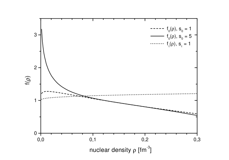
FIG. 1.: Density dependent isoscalar f₀ (s${}_{0}=1$ dashed line, s${}_{0}=5$ solid line) and isovector f_τ (dotted line) vertex functions of the D3Y interaction.

Fig. 1 shows the density dependence of the vertex correction functions f₀ and f_τ. In the isovector channel only a rather small deviation from unity is found, and f_τ increases only slightly for higher densities. This reflects the fact that the original interaction already has a symmetry coefficient close to 32 MeV. In the isoscalar channel one realizes an increase of the interaction at low densities and a suppression of the interaction at higher densities. The low density behavior obviously scales with s₀. In Fig. 2 the equations of state (EoS) for the D3Y and the Skyrme SLy4 interaction [36] are compared. For s₀=1 the D3Y and the SLy4 results are in very close agreement over the full range of densities. According to the behavior of f₀, the binding energy increases at densities lower and decreases at densities higher than the saturation density for s${}_{0}>$1 while retaining its value at the equilibrium density.

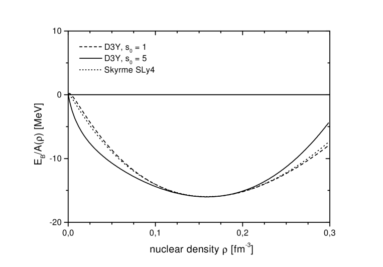
FIG. 2.: Nuclear matter equation of state calculated with the density dependent D3Y interaction for the parameterizations s${}_{0}=1$ (dashed line) and s${}_{0}=5$ (solid line) and the Skyrme SLy4 interaction (dotted line).

The isovector properties of the D3Y interactions are illustrated in Fig. 3, where the EoS for asymmetric nuclear matter is displayed for different asymmetry ratios $Z/A=\rho_{p}/\rho$. Stable nuclei typically cover the range $Z/A=0.5\dots 0.4$ (e.g. ⁴⁰Ca, ²⁰⁸Pb). In exotic nuclei the new regions with $Z/A=0.4\dots 0.3$ become accessible and far of stability $Z/A=0.2$ may be reached (e.g ¹⁰He). It is remarkable that neutron matter is still bound but this occurs at extremely low densities. The reason for this behavior is the strong attraction of the D3Y with s${}_{0}=5$ at very low densities and, as such, is not very conclusive. In stable nuclei these density regions will rarely contribute to the total binding. However, a different situation may be expected far off stability, especially in halo nuclei, where the binding sensitively depends on the interactions at low density. Comparing the D3Y to the SLy4 interaction one sees that both interactions are in agreement around the saturation density for asymmetry ratios of $Z/A=0.5\dots 0.4$. The differences showing up at low densities and large asymmetries are mainly due to the stronger attraction of the D3Y isoscalar interaction with s₀=5.

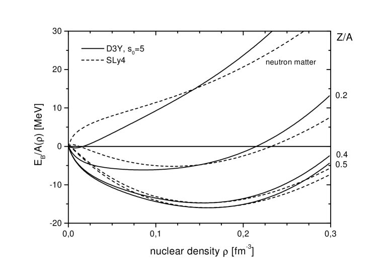
FIG. 3.: Equation of state for asymmetric nuclear matter calculated with the density dependent D3Y interaction for the parameterizations s${}_{0}=5$ (solid line) and the Skyrme SLy4 (dashed line). Shown is the EoS for neutron matter and for the asymmetry ratios $Z/A=0.2,0.4,0.5$.

In Fig. 4 the EoS for different asymmetry ratios and the two sets of parameters are examined. The equilibrium density $\rho_{0}(\xi)$, the energy per nucleon $E_{B}(\xi)/A$, the symmetrie energy $\epsilon_{\tau}(\xi)$ and the compressibility K_∞($\xi$) for $\xi$=Z/A are shown. A higher value of s₀ is seen to lead to a lower equilibrium density for strong asymmetries. In addition the binding energy at the equilibrium density is higher due to the stronger attraction of this parameterization of the interaction at low densities. The lower left part shows the symmetry energy of the EoS in dependence of the proton excess. One realizes a decrease of the symmetry energy for strong asymmetries and a higher value of s₀ corresponding to the shift of the saturation density to lower densities. The compressibility approaches zero at high asymmetries with a remarkable flat slope.

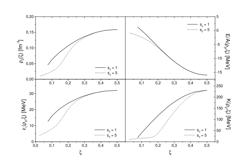
FIG. 4.: Equilibrium density $\rho_{0}$ of the EoS (upper left), binding energy per nucleon $E_{B}/A$ at $\rho_{0}$ (upper right), symmetry coefficient $\epsilon_{\tau}$ at $\rho_{0}$ (lower left) and the compressibility K_∞($\rho_{0}$) (lower right ), all plotted as a function of the neutron excess or asymmetry ratio $\xi=Z/A$. Results are shown for the D3Y interaction with s${}_{0}=1$ and s${}_{0}=5$.

The properties of the D3Y interaction in the particle-particle channel were investigated by considering like–particle pairing in symmetric nuclear matter. Pairing, being mediated by the singlet-even part $V_{SE}$ of the interaction, was examined by Hartree-Fock-Bogoliubov (HFB) calculations. The in–medium SE particle–particle interaction was obtained by back transformation from the renormalized particle–hole interactions using the representation in terms of the exchange interactions (see App. A), leading to $V_{SE}^{*}(\rho)=2\sum_{\gamma=0,\tau}\left[V_{\gamma}^{*d}(\rho)+V_{\gamma}^{*e}(\rho)\right]$.

As in refs. [37, 38] the following set of equations was solved simultaneously:

$$\rho(k_{F}) = 4\int\frac{d^{3}k}{(2\pi)^{3}}v^{2}(k,k_{F})$$ (53)

$$v^{2}(k,k_{F}) = \frac{1}{2}\left\{1-\frac{\epsilon(k,k_{F})-\lambda}{\sqrt{(\epsilon(k,k_{F})-\lambda)^{2}+\Delta^{2}(k,k_{F})}}\right\}=1-u^{2}(k,k_{F})$$ (54)

$$\epsilon(k,k_{F}) = \frac{\hbar^{2}k^{2}}{2m}+4\int\frac{d^{3}k^{\prime}}{(2\pi)^{3}}\langle kk^{\prime}|V^{*}|kk^{\prime}-k^{\prime}k\rangle v^{2}(k^{\prime},k_{F})$$ (55)

$$\Delta(k,k_{F}) = -\int\frac{d^{3}k^{\prime}}{(2\pi)^{3}}\langle k-k|V_{SE}^{*}|k^{\prime}-k^{\prime}\rangle u(k^{\prime},k_{F})v(k^{\prime},k_{F})$$ (56)

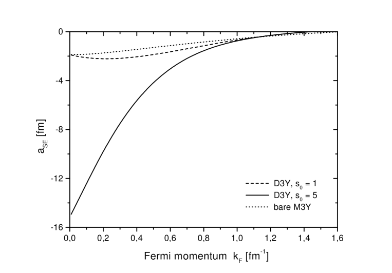
FIG. 5.: Scattering length $a_{SE}^{pp}(k_{F})$ for relative s–wave states. Results are shown for the bare M3Y (dotted) and the D3Y with the parameterizations s${}_{0}=1$ (dashed line) and s${}_{0}=5$ (solid line).

Fig. 5 shows the calculated in–medium scattering length for like particles (pp/nn) $a_{SE}^{pp}(k_{F})$ at a given Fermi momentum $k_{F}$ for different parameterizations of the interaction. Because of the density dependence in the isovector and in the isoscalar channel the strength of the interaction increases at low to intermediate densities. For the D3Y with s${}_{0}=5$ the pairing interaction is enhanced by a factor of about 8 at low densities over the values of the original M3Y because of the asymptotic scaling of the isoscalar interaction. This corresponds to about 90% of the s-wave strength of the free NN T-matrix with a scattering lenght of $a_{SE}^{pp}=-17.1$fm and leads to higher values of the gap in nuclear matter. In Fig. 6 $\Delta(k,k_{F})$ at k=k_F is shown. For the bare M3Y the position of the maximum gap lies at about k${}_{F}\simeq$0.8 fm^-1. About the same result is obtained in HFB calculations with the Gogny force [37, 38] and for several Skyrme interactions [39]. The position of the maximum gap in the D3Y–calculations is shifted to slightly lower densities with $k_{F}\simeq$=0.75 fm^-1 resp. k${}_{F}\simeq$0.63 fm^-1 for s₀=1 resp. s₀=5. One finds that the height of the maximum increases by lowering the position of the maximum. Our results of $\Delta(k_{F},k_{F})\simeq 2$ MeV resp. $\Delta(k_{F},k_{F})\simeq 4$ MeV for the M3Y and the D3Y with s${}_{0}=1$ are in agreement with the Gogny force that yields a value of $\Delta(k_{F},k_{F})\simeq 3$ MeV [37, 38]. The calculated maximum gap for the D3Y with s${}_{0}=5$ has a much higher value of about 9.5 MeV. The reason for this is the much stronger pairing interaction, especially at lower densities, as seen in Fig. 5. Comparing the value of the gap at the saturation density $k_{F}=1.33fm^{-1}$ with other calculations we find a value of about 0.2 MeV for the M3Y and a nearly vanishing value for the D3Y interaction. For the Gogny force one finds a value of about 0.6 MeV but most other calculations favor a small to vanishing gap [39, 40, 41].

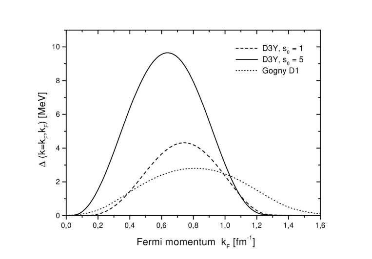
FIG. 6.: Gap at the Fermi momentum in nuclear matter. Results for the D3Y interaction with s${}_{0}=1$ (dotted line) and s${}_{0}=5$ (solid line) and the Gogny D1 (dashed line) are shown.

IV Hartree–Fock Calculations for Finite Nuclei

The density dependent D3Y interaction derived in the preceding section for nuclear matter is applied in HF–calculations for finite nuclei. Stable nuclei close to the N$\simeq$Z line are chosen first. In these calculations mainly the isoscalar properties of the interaction are investigated. A more general test, including also isovector dynamics, is obtained from calculations for even-even Sn–isotopes covering the range from the proton dripline (¹⁰⁰Sn) to the A=140 mass region. The calculations for stable and unstable nulcei are performed without readjustment of parameters from their values derived for nuclear matter.

The general structure of the HF–equations for a density dependent NN-interaction in the DME approach was already derived in Sect. II B. In the practical applications the DME is used only for the exchange contributions to the HF potentials. Especially at higher density and thus Fermi momentum exchange is dominated by the short range pieces of the interaction for which the local momentum approximation underlying the DME is most appropriate. Different from the original work of Negele and Vautherin [8] the direct, i.e. Hartree potentials are treated in full finite range.

The D3Y density dependence was introduced as a local renormalization of the vertices which requires to replace the interaction by [18]

$$V^{*d}_{\gamma}({\bf r}_{1},{\bf r}_{2};\rho)=g_{\gamma}({\bf r}_{1})V^{d}_{\gamma}({\bf r}_{1}-{\bf r}_{2})g_{\gamma}({\bf r}_{2})$$ (57)

with $g^{2}_{\gamma}=f_{0,\tau}$ and where $g_{\gamma}({\bf r})=g_{\gamma}(\rho({\bf r}))$ are the in–medium isoscalar and isovector vertex renormalizations, respectively. $V^{d}_{\gamma}({\bf r}_{1}-{\bf r}_{2})$ denotes the unrenormalized ”bare” interaction in these channels. This ensures a reliable treatment of the density dependence also in the surface region where the vertices vary rapidly (see Fig. 1). The direct potentials are obtained as in Eq.(18) by folding the proton and neutron densities, respectively, with the corresponding – now density dependent – direct interactions. To accomplish this we express the interactions $V_{qq^{\prime}}^{d}({\bf r}_{1},{\bf r}_{2})$ by $V^{*d}_{\gamma}({\bf r}_{1},{\bf r}_{2};\rho)$. With the DME the exchange or Fock potentials are replaced by local potentials whose strengths are defined in Eq.(11). In order to preserve this separation of the center–of–mass and relative coordinates ${\bf r}$ and ${\bf s}$ the interaction must also be separable in ${\bf r}$ and ${\bf s}$. Assuming that the resulting error is small compared to the error introduced by the DME we therefore replace in the exchange interaction, as a first approximation, the individual coordinates of the interacting particles by their center–off–mass coordinate. This leads to

$$V^{*e}_{\gamma}({\bf s},{\bf r};\rho)=g^{2}_{\gamma}({\bf r})V^{e}_{\gamma}({\bf s})$$ (58)

by which we express the exchange interactions $V_{qq^{\prime}}^{e}({\bf s})$.

A Details Of Numerical Calculation

For our calculations we only consider the stationary ground state of spherical even-even nuclei, therefore the single particle wave functions can be separated as

$$\phi_{k_{q}}({\bf r})=\frac{R_{\alpha_{q}}(r)}{r}\Psi_{ljm}(\theta,\phi)$$ (59)

The functions $\Psi_{ljm}(\theta,\phi)$ are spinor spherical harmonics [42], the index $\alpha_{q}$ represents the quantum numbers $\alpha_{q}=\{n,l,j\}$ for protons and neutrons, resp. This allows us to simplify the density and the kinetic energy density to

$$\rho_{q}(r) = \frac{1}{4\pi r^{2}}\,\sum_{\alpha_{q}}\,v_{\alpha_{q}}^{2}(2j_{\alpha_{q}}+1)R_{\alpha_{q}}^{2}(r)$$ (60)

$$\tau_{q}(r) = \frac{1}{4\pi}\,\sum_{\alpha_{q}}\,v_{\alpha_{q}}^{2}(2j_{\alpha_{q}}+1)\left[\left(\partial_{r}\frac{R_{\alpha_{q}}(r)}{r}\right)^{2}+\frac{l_{\alpha_{q}}(l_{\alpha_{q}}+1)}{r^{2}}\,\left(\frac{R_{\alpha_{q}}(r)}{r}\right)^{2}\right]$$ (61)

The occupation weights $v_{\alpha_{q}}^{2}$ for a state $\alpha_{q}$ are determined by pairing correlations. Since it was found that pairing gives minor to negligible contributions to the nuclei considered here, the BCS approximation was used. A constant pairing matrix element of $G_{q}=23$ MeV/nucleon was used and the standard set of BCS equations [20] was solved independently for protons and neutrons, respectively.

For protons also the Coulomb interaction contributes to the Hartree–Fock potential $U^{HF}$:

$$U_{Coul}({\bf r})=\int d^{3}r_{1}\,\rho_{p}({\bf r}_{1})\,\frac{e^{2}}{|{\bf r}-{\bf r}_{1}|}\,\,\,\,-\,\,\,\,\left(\frac{3}{\pi}\right)^{1/3}e^{2}\rho_{p}({\bf r})^{1/3}$$ (62)

The Coulomb exchange term is treated in the local density approximation rather than in the full DME because its contribution to the potential energy is small.

The spin-orbit potential is treated as in [8, 43], leading to a contribution to the potential energy $E_{s.o.}=\int d^{3}r\,H_{s.o.}({\bf r})$ with

$$H_{s.o.}({\bf r}) = -\frac{1}{2}W_{0}\left\{\rho({\bf r})\,{\bf\nabla}{\bf J}({\bf r})+\sum_{q}\rho_{q}({\bf r})\,{\bf\nabla}{\bf J}_{q}({\bf r})\right\}.$$ (63)

The spin-orbit strength $W_{0}$ is related to the two-body spin-orbit potential in the short–range limit by

$$W_{0}=-\frac{2\pi}{3}\int V_{LS}(s)s^{4}\,ds$$ (64)

Using the M3Y parameterization [21] one finds a value of $W_{0}\sim 105$ MeV fm⁵ but in correspondence to most Skyrme interactions $W_{0}=120$ MeV fm⁵ from reference [43] is chosen. After variation this term gives a contribution

$$U_{q}^{s.o.}({\bf r})=-\frac{1}{2}W_{0}\left[\rho({\bf r})\,{\bf\nabla}{\bf J}({\bf r})+\rho_{q}({\bf r})\,{\bf\nabla}{\bf J}_{q}({\bf r})\right],$$ (65)

to the Hartree–Fock potential and a single particle spin-orbit potential

$$U_{q}^{{\bf l}{\bf s}}(r)=\frac{1}{2}W_{0}\frac{1}{r}\,\frac{d}{dr}\,\left[\rho(r)+\rho_{q}(r)\right]{\bf l}\cdot{\bf s}$$ (66)

where the spin density is defined as

$$J_{q}(r)=\frac{1}{4\pi r^{3}}\,\sum_{\alpha_{q}}\,(2j_{\alpha_{q}}+1)\left[j_{\alpha_{q}}(j_{\alpha_{q}}+1)-l_{\alpha_{q}}(l_{\alpha_{q}}+1)-\frac{3}{4}\right]R_{\alpha_{q}}^{2}(r).$$ (67)

B Results for Stable Nuclei

The various contributions to the nuclear part of the self–consistent DME mean–field in ⁴⁰Ca are shown in Fig. 7. The isoscalar Hartree potential is weak and repulsive and binding is essentially mediated by the Fock parts. The Fock potential is strongly attractive with a depth at the center of about -110 MeV. The sum of the Hartree and Fock terms leads to an average potential depth of -70 MeV. The direct and exchange rearrangement potentials reduce the depth especially close to the center. The mean–field agrees qualitatively with other non–relativistic HF results, e.g [43]. It also resembles closely the Schroedinger-equivalent potential from a relativistic density dependent Hartree calculation [17, 18] except for a more pronounced shell structure.

Of special interest is the influence of the rearrangement potential whose influence has proven to be important as found in comparable non-relativistic [43] and relativistic calculations [17, 18]. Rearrangement is of importance for the single particle potential and the energy spectrum. Because the rearrangement potential is always repulsive it lowers the single particle potential and leads to a change in the single particle spectra and the charge radii. In the calculation of the total binding energy the rearrangement effects cancel out. Taking this into account the total binding energy is given as

$$E_{B}=\sum_{i=1}^{A}\epsilon_{i}-\frac{1}{2}\sum_{q=p,n}\int d^{3}r\rho_{q}(r)U^{HF}_{q}(r)-\sum_{q=p,n}E_{q}^{R}+E_{pair},$$ (68)

with the rearrangement energy calculated from Eq.(30) and Eq.(32):

$$E_{q}^{R}=\int d^{3}r\,\rho_{q}(r)\,U^{R}_{q}(r)+\int d^{3}r\,\tau_{q}(r)\,\frac{\hbar^{2}}{2}\left(\frac{1}{m_{q}^{*}(r)}-\frac{1}{m}\right)$$ (69)

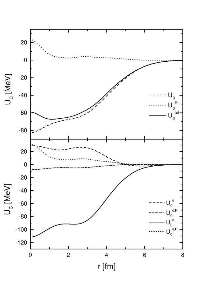
FIG. 7.: Single particle potential for ⁴⁰Ca calculated with the D3Y with $s_{0}=5$. In the lower part, contributions to the total isoscalar potential from the direct $U_{0}^{d}$ and the exchange term $U_{0}^{e}$ of the normal Hartree-Fock potential as well as the rearrangement potentials ($U_{0}^{d,R}$, $U_{0}^{e,R}$) are shown. In the upper part, the total isoscalar potential $U_{0}^{tot}$ as well as its contributions, the attractive HF potential $U_{0}$ and the repulsive rearrangement potential $U_{0}^{R}$, are shown.

An important contribution to mean–field dynamics is provided by the momentum dependence of the interaction. Since the exchange parts of the D3Y interaction were found to be most important for nuclear binding the question arises whether the momentum structure is described realistically. The effective mass m${}^{*}_{q}$, Eq.(30) is completely determined by the Fock terms, since they are the only source of non–localities in the present model. From Fig. 8 it is seen that a very reasonable value of about $m^{*}_{q}/m\simeq$0.68 is obtained in the interior of a heavy nucleus like ²⁰⁸Pb which closely agrees with other theoretical results and determinations from proton–nucleus elastic scattering [44]. It is worthwhile to emphasize that this result was obtained without readjustments of parameters. The D3Y interaction (or better to say the original M3Y G–matrix [21]) has apparently a realistic mixture of short and long range contributions accounting reasonably well for the intrinsic momentum structure of an in–medium HF interaction. The results of this section also confirm the DME approach. Especially promising results are obtained in conjunction with the effective ”Fermi momentum” q_F, Eq.(9), by which non–local effects are accessible in a self–consistent way.

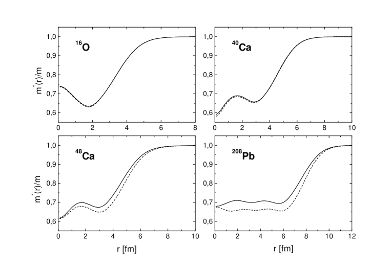
FIG. 8.: Effective mass of protons (solid line) and neutrons (dashed line) in closed shell nuclei calculated with the density dependent D3Y interaction (with the parameterization $s_{0}=5$.)

TABLE III.: Charge radii $r_{C}$ [fm] for closed shell nuclei for different parameterizations of the D3Y interaction

	16O	40Ca	48Ca	208Pb
$s_{0}=1$	2.79	3.51	3.52	5.51
$s_{0}=5$	2.88	3.61	3.60	5.59
exp.	2.73	3.49	3.47	5.50

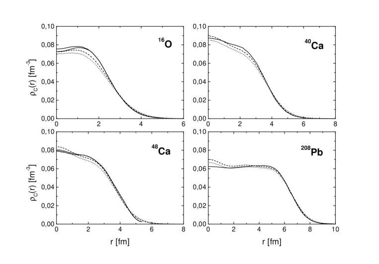
FIG. 9.: Charge density distributions of closed shell nuclei from density dependent Hartree-Fock calculations using the D3Y interaction. Results for $s_{0}=1$ (dashed line) and $s_{0}=5$ (dotted line) are shown. Experimental densities and their uncertainties are denoted by solid lines (taken from Ref. [45]) .

Fig. 9 compares the calculated charge density distributions of the above closed–shell nuclei with experimental data from elastic electron scattering [45]. The theoretical point particle distribution was folded with a Gaussian proton form factor [43] with $\sqrt{\langle r^{2}\rangle_{p}}=0.8fm$. Tab. III shows the calculated charge radii in comparison to the experimental data (taken from [18]).

The charge density in the nuclear interior is slightly overestimated for heavy nuclei like ²⁰⁸Pb and slightly underestimated for the lighter nuclei. In all cases, the density at large radii is higher than the experimental data which leads to a overestimation of charge radii as can be seen in Tab. III. In general the agreement with the experimental charge radii is satisfying and is, except for ¹⁶O, $\leq 2\%$ for the D3Y with $s_{0}=1$ and $\leq 4\%$ for the D3Y with $s_{0}=5$. In contrast to this, the binding energies calculated with $s_{0}=1$ are strongly underestimated by more than 0.5 MeV per nucleon, whereas the D3Y with $s_{0}=5$ reproduces the experimental data [46] very well (Tab. IV). One sees that an improvement in the binding energies leads to higher values of the charge radii. In general it is not possible to reproduce simultaneously both the binding energies and the charge radii with one parameter set. This is in agreement with calculations in the relativistic density dependent field theory which typically give comparable results [13, 15]. But generally the agreement with the experimental binding energies of the D3Y with $s_{0}=5$ is surprisingly good as can be seen in Fig. 10 realizing that the number of used parameters is lower than the one in Gogny or Skyrme interactions.

The observed behavior of the D3Y for different parameterizations shows the importance of the density dependence of the interaction. Although both parameterizations have the same properties in the range of the saturation density in nuclear matter the results for finite nuclei are quite different. This behavior is caused by the differences at low densities. In addition, the rearrangement terms enhance the effect of the density dependence.

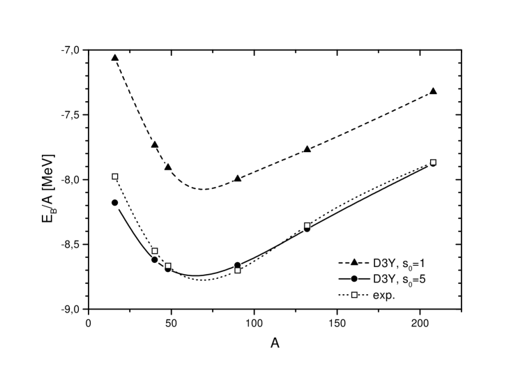
FIG. 10.: Binding energy per nucleon for closed shell nuclei from density dependent Hartree-Fock calculations using the D3Y interaction. Results for $s_{0}=1$ (triangles) and $s_{0}=5$ (circles) are shown. Experimental binding energies are denoted by open squares (taken from Ref. [46]). Binding energies are shown for the nuclei ¹⁶O, ⁴⁰Ca, ⁴⁸Ca, ⁹⁰Zr, ¹³²Sn and ²⁰⁸Pb. Lines are drawn to guide the eye.

TABLE IV.: Binding energy per nucleon $E_{B}/A$ [MeV] for closed shell nuclei for different parameterizations of the D3Y interaction

	16O	40Ca	48Ca	90Zr	132Sn	208Pb
$s_{0}=1$	-7.07	-7.74	-7.91	-8.00	-7.77	-7.32
$s_{0}=5$	-8.18	-8.62	-8.69	-8.66	-8.38	-7.88
exp.	-7.98	-8.55	-8.67	-8.70	-8.36	-7.87

C The Ground States of Sn Isotopes

The Sn isotopes are of particular interest for nuclear structure and also astrophysical questions because of the closure of the Z=50 proton shell. The known isotopes [46] cover the range from the proton dripline at ¹⁰⁰Sn [47] to the doubly magic ¹³²Sn nucleus which is already $\beta$–unstable. Here, we are mainly interested to investigate the isovector properties of the D3Y interaction and, as a more general aspect, to test an effective interaction, determined from symmetric nuclear matter and stable nuclei, in regions far off stability. No attempt is made to optimize the parameters in order to obtain a perfect fit of data. The parameter set with s₀=5 is used.

Theoretical and experimental binding energies per particle are compared in Fig. 11. The D3Y binding energies are seen to be shifted slightly to the left of the data [46] but a fair description of the overall dependence on mass and asymmetry is obtained. The strongest binding is obtained for ¹²⁰Sn while experimentally the minimum is found at approximately ¹¹⁵Sn. The binding energies of the neutron–rich isotopes are reasonably well reproduced but in view of the deviations on the neutron–poor side the agreement might be fortuitous. Towards the proton dripline, i.e. N$\rightarrow$Z, the binding energies are increasingly underestimated by up to about 0.12 MeV per nucleon close to ¹⁰⁰Sn. This result is to some extent unexpected because stable nuclei with N$\sim$Z were well described. However, also the binding energy of ⁹⁰Zr (Fig. 10 is underestimated the most and apparently the effect is enhanced in going from the N=50 to the Z=50 shell. The deviations are in a range typical for calculations with a G–matrix in finite nuclei. Fully phenomenological interactions like the Skyrme SLy4 force, for which results are also displayed in Fig. 11, and the Gogny D1 interaction [19] reproduce the Sn binding energies almost perfectly.

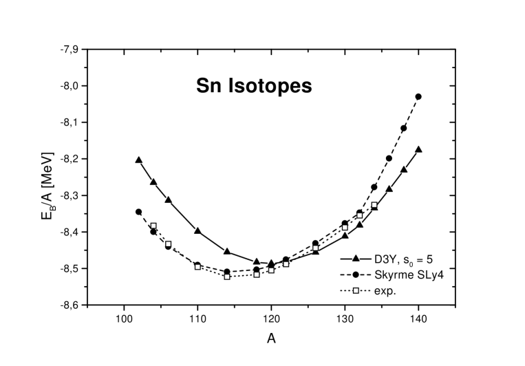
FIG. 11.: Binding energy per nucleon for the tin isotopes from density dependent Hartree-Fock calculations using the D3Y interaction with $s_{0}=5$ (triangles) and the Skyrme SLy4 force [36] (cirles). Experimental binding energies are denoted by open squares (taken from Ref. [46]). The lines are drawn to guide the eye.

Variations of the scaling parameter s₀ resulted in an overall shift of the binding energy curve as it might be expected. Improvements on the neutron–poor side are obtained on the expense of a worse description of the neutron–rich isotopes. In particular, the minimum was found to be rather insensitive on variations of s₀. For s₀=1 the whole curve is shifted up by about 0.5 MeV per nucleon with essentially the same shape. These observations lead to the conclusion that the parameters a${}^{0}_{n}$ themselves should be readjusted on finite nuclei with constraints to nuclear matter rather than retaining the nuclear matter values. Taking the point of view that the nuclear matter parameterization accounts for the static part of the interaction, where cluster contributions are included effectively by the fitting procedure [27], such a refinement could be related to non–static contributions to the in–medium interaction because of the larger polarizability of the nuclear surface. Theoretically, this would amount to go beyond the ladder approximation and to include also ring diagrams. Such contributions are obviously contained in e.g. the Skyrme parameters but missing in the D3Y interaction. Over the range of the Sn isotopes the polarization contributions can be expected to decrease towards A$\sim$132 which is known to be a rather stiff nucleus.

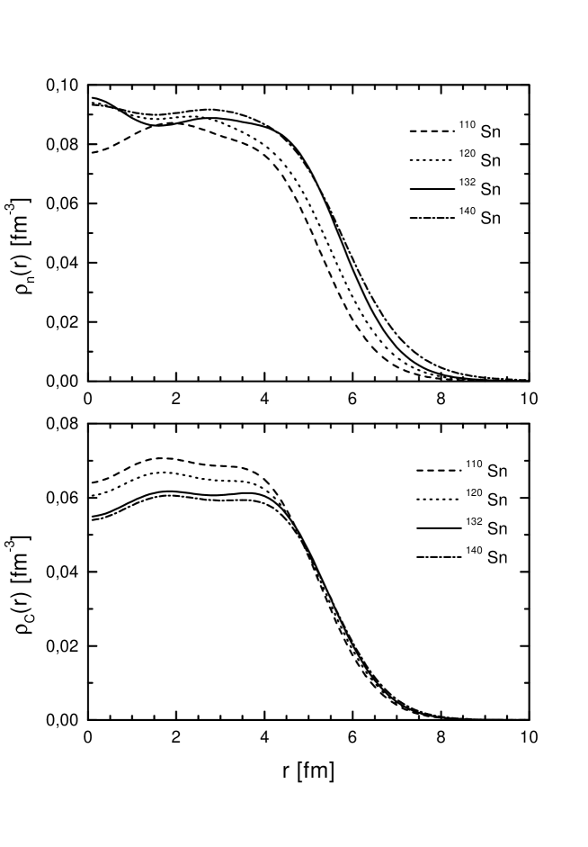
FIG. 12.: Charge density distributions (lower part) and neutron density distributions (upper part) of the tin isotopes from density dependent Hartree-Fock calculations using the D3Y interaction. Results for $s_{0}=5$ are shown.

Neutron density distributions and charge densities for several Sn isotopes are displayed in Fig. 12. From ¹¹⁰Sn to ¹⁴⁰Sn the charge distributions are slightly reduced in the interior. As seen in Fig. 13 this is accompanied by a mild increase of the charge radius by about 5%. A more drastic evolution is found for the neutron densities. Beyond ¹³²Sn an extremely thick neutron skin is building up leading to a sudden jump in the neutron rms radii. The neutron skin thickness is more clearly visible in Fig. 14 where the difference of the proton and neutron rms radii is shown. In ¹⁴⁰Sn a solid layer of neutron matter is found extending by about 0.48 fm beyond the proton matter distribution which is more than a factor of two larger than the neutron skin in ²⁰⁸Pb. The same phenomenon is predicted also by the SLy4 interaction except for a somewhat smaller neutron excess radius. The saturation of the rms values around A=132 is an indication of the double magic nature of ¹³²Sn. The increase is directly related to the shell structure in the heavy tin isotopes. At A=132 the 2f_7/2 shell is filled and pairing does not contribute. At larger masses the neutron 3p–subshells become populated. Weak binding and the low angular momentum barrier allow a large extension of the valence wave functions into the exterior. However, the calculations do not lead to a ”halo”.

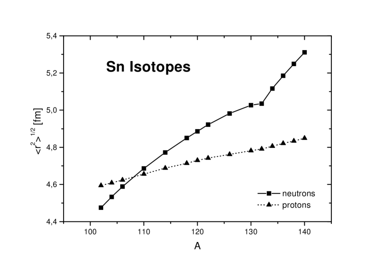
FIG. 13.: Root mean square radii of the tin isotopes from density dependent Hartree-Fock calculations using the D3Y interaction with $s_{0}=5$ for neutrons (squares) and protons (triangles). The lines are drawn to guide the eye.

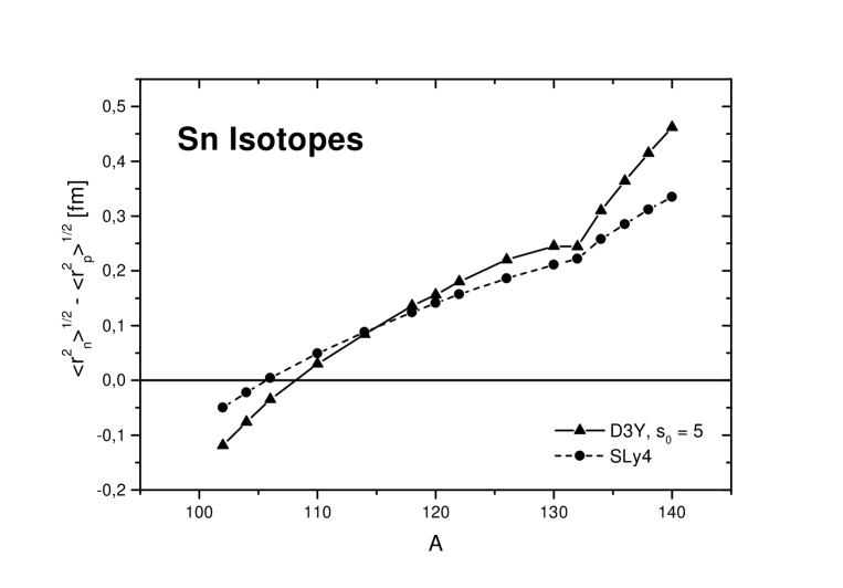
FIG. 14.: Difference of the root mean square radii of neutrons and protons of the tin isotopes for the D3Y interaction with $s_{0}=5$ (triangles) and the Skyrme SLy4 (cirles). The lines are drawn to guide the eye.

An interesting observation is made from Fig. 14 on the neutron–poor side. Both the D3Y and the SLy4 interactions predict a proton skin for A$\leq$106. The origins of the proton and neutron skins are quite different. Atthe neutron rich side the excess neutrons become less bound because of the increasing repulsion from the isovector potential. Since states with $\ell\geq$1 are involved they are stored predominantly in the surface region of the nucleus. In the heavy isotopes the isovector potential acts attractively in the proton sector and thus balances to a large extent the Coulomb repulsion. Since for N$\rightarrow$Z the isovector part of the mean–field becomes strongly suppressed the repulsion is no longer compensated and Coulomb effects become visible. Hence, the proton skin in the neutron–poor Sn nuclides is caused solely by the Coulomb interaction.

The calculations were extended further into the $\beta$–unstable region. Up to A=160 the neutron dripline is still not reached. The separation energies are small but decrease rather slowly.

V Summary, Discussion and Conclusions

The density matrix expansion (DME) method was used to derive a local energy density functional for non–relativistic meson exchange interactions. The interaction energy density was separated into direct and exchange contributions. The Hartree contributions are treated exactly. From the systematic expansion of the one–body density matrix provided by the DME an average momentum density was determined such that the next to leading order terms in the DME series are canceled. In uniform systems like infinite nuclear matter all higher order terms are canceled and the exact energy density is recovered. In finite nuclei the approach corresponds to a generalized Slater expansion of the density matrix. Hartree–Fock equations were derived. With our choice for q${}^{2}_{F}$ a self–consistently generated effective mass was obtained which is completely determined by the intrinsic momentum structure of the underlying interaction.

A semi–microscopic approach to the in–medium NN interaction was discussed. The M3Y G–matrix from the Paris NN potential was modified by introducing density dependent vertex renormalizations in the isoscalar and isovector particle–hole channels. The functional form of the vertex functions was chosen in close analogy to the dynamical structure and the medium dependence of the vertices in a Brueckner G–matrix. The parameters, however, were determined empirically by a fit to the binding energy, equilibrium density, compressibility and the symmetry energy of symmetric nuclear matter. The momentum structure of the original G–matrix was retained.

The probably first attempt to parameterize a G–matrix in terms of fixed propagators and density dependent vertices goes back to Sprung and Banerjee [48]. They approximated the momentum structure of the singlet/triplet even-odd interactions obtained from the Reid NN potential by a superposition of 5 arbitrarily chosen gaussians with channel dependent in–medium vertices. The functional form of the vertices was chosen in the same way as in section III A but using always a first order polynomial. The nuclear matter binding energy curve of the full Reid G–matrix was reproduced the best for a linear dependence of the vertices on k_F, corresponding to $\beta$=1/3 in Eq.(40). From the description of individual matrix elements a slight preference for a lower value $\beta$=1/6 was deduced [48]. However, nuclear matter was found to be badly underbound by about 5 MeV since only two-body correlations were taken into account. The renormalized vertices obtained in our semi–microscopic approach include effectively also contributions beyond the two–body cluster approximation, as was pointed out some time ago by Bethe [27].

In nuclear matter the D3Y interaction leads to an equation of state with an unusual enhancement of attraction at low densities which is not found for phenomenological forces. Unfortunately, G–matrix calculations are not available at such low densities but obviously the free NN T–matrix should be approached asymptotically. Phenomenological interactions and also the unrenormalized M3Y G–matrix do not account for this transition. Without putting too much emphasis on the details of this particular result it might be expected that such a region of enhanced attraction could indeed exist in the far tails of nuclear wave functions. Before drawing final conclusions on this subject a refined treatment of the low density region is clearly necessary. For that purpose an extended version of the schematic model for the in–medium vertices might prove to be useful.

The ground state properties of stable nuclei were reproduced reasonably well. The good description of binding energies gives confidence to the DME approach, especially in view of the fact that an interaction from nuclear matter was used.

Acknowledgement:

This work was supported in part by DFG (contract Le439/4-1), GSI and BMBF.

A Representations Of The NN Interaction

In literature several representations of the NN interaction exist which can be found in, e. g. [22]. Here we will only consider the central part of the interaction. The M3Y interaction is given in a representation specifying the two-body channel spin and the parity (SE,TE,SO,TO) which is commonly used in inelastic scattering. In our calculations we are especially interested in the p-p resp. p-n interaction for calculating the Hartree-Fock matrix elements, the (pp, pn) representation. It can be easily obtained with the transformation [49]

$$V_{pp}^{d} = \frac{1}{8}\left[2V_{SE}+6V_{TO}\right]=V_{nn}^{d}$$ (A1)

$$V_{pn}^{d} = \frac{1}{8}\left[1V_{SE}+3V_{TE}+1V_{SO}+3V_{TO}\right]=V_{np}^{d}$$ (A2)

$$V_{pp}^{e} = \frac{1}{8}\left[2V_{SE}-6V_{TO}\right]=V_{nn}^{e}$$ (A3)

$$V_{pn}^{e} = \frac{1}{8}\left[1V_{SE}+3V_{TE}-1V_{SO}-3V_{TO}\right]=V_{np}^{e}$$ (A4)

Here, the indices $d$ resp. $e$ stand for the direct resp. exchange part of the NN interaction. A representation especially useful if one uses a contact interaction or is interested in the direct part of the interaction is the set ($V_{0},V_{\sigma},V_{\tau},V_{\sigma\tau}$), which follows from the set (SE,TE,SO,TO) through

$$V_{0} = \frac{1}{16}\left[3V_{SE}+3V_{TE}+1V_{SO}+9V_{TO}\right]$$ (A5)

$$V_{\sigma} = \frac{1}{16}\left[-3V_{SE}+1V_{TE}-1V_{SO}+3V_{TO}\right]$$ (A6)

$$V_{\tau} = \frac{1}{16}\left[1V_{SE}-3V_{TE}-1V_{SO}+3V_{TO}\right]$$ (A7)

$$V_{\sigma\tau} = \frac{1}{16}\left[-1V_{SE}-1V_{TE}+1V_{SO}+1V_{TO}\right]$$ (A8)

Our aim is to find a spin averaged interaction which separates the isoscalar and the isovector interaction for both the direct and the exchange part. Defining

$$V_{0}^{d/e} = \frac{1}{4}(V_{pp}^{d/e}+V_{pn}^{d/e}+V_{np}^{d/e}+V_{nn}^{d/e})$$ (A9)

$$V_{\tau}^{d/e} = \frac{1}{4}(V_{pp}^{d/e}-V_{pn}^{d/e}-V_{np}^{d/e}+V_{nn}^{d/e})$$ (A10)

we find in the (SE,TE,SO,TO) representation

$$V_{0}^{d} = \frac{1}{16}\left[3V_{SE}+3V_{TE}+1V_{SO}+9V_{TO}\right]=V_{0}$$ (A11)

$$V_{\tau}^{d} = \frac{1}{16}\left[1V_{SE}-3V_{TE}-1V_{SO}+3V_{TO}\right]=V_{\tau}$$ (A12)

$$V_{0}^{e} = \frac{1}{16}\left[3V_{SE}+3V_{TE}-1V_{SO}-9V_{TO}\right]$$ (A13)

$$V_{\tau}^{e} = \frac{1}{16}\left[1V_{SE}-3V_{TE}+1V_{SO}-3V_{TO}\right].$$ (A14)

One sees that the defined direct terms of this representation are equivalent to the ones of the set ($V_{0},V_{\sigma},V_{\tau},V_{\sigma\tau}$) but also that there is no equivalent for the exchange terms.

REFERENCES

- [1] W. Schwab, H. Geissel, H. Lenske, K.-H. Behr, A. Brünle, K. Burkhard, H. Irnich, T. Kobayashi, G. Kraus, A. Magel, G. Münzenberg, F. Nickel, K. Riisager, C. Scheidenberger, B. M. Sherill, T. Suzuki, B. Voss, Z.Phys. A350 (1995) 283.
- [2] M. Zinser, H. Emling, H. Lenske et al., Nucl.Phys A (in print); N. Ostrowski. H. G. Bohlen, A. S. Demyanova, B. Gebauer, R. Kapakchieva, Ch. Langner, H. Lenske, M. von Lucke-Petsch, W. von Oertzen, A. A. Ogloblin, Y. E. Penionzhkevich, M. Wilpert and Th. Wilpert, Z.Phys. A343 (1992) 389; H. G. Bohlen, B. Gebauer, M. von Lucke-Petsch, W. von Oertzen, A. N. Ostrowski and H. Lenske, Z.Phys. A344 (1993) 381.
- [3] T. H. R. Skyrme, Nucl. Phys. 9 (1959) 615.
- [4] K. A. Brueckner, J.R. Buchler, S. Jorna and R.J. Lombard, Phys. Rev. 171(1968) 1188.
- [5] H. S. Koehler, Phys. Rep. 18C (1975) 219.
- [6] R. K. Tripathi, A. Faessler, and H. Müther, Phys. Rev. C10 (1974) 2080.
- [7] H. Kümmel, K. H. Lührmann and J. G. Zabolitzky, Phys. Rep. 36 (1978) 1.
- [8] J. W. Negele and D. Vautherin, Phys. Rev. C5 (1972) 1472.
- [9] J. W. Negele, Rev. Mod. Phys. 54 (1982) 913.
- [10] F. T. Baker, L. Bombot, C. Djalali, C. Glashauser, H. Lenske, W. G. Love, M. Morlet, E. Tomasi–Gustafson, J. Van der Wiele, J. Wambach, A. Willis, Phys.Rep. (in print).
- [11] M. R. Anastasio, L. S. Celenza, W. S. Pong and C. M. Shakin, Phys. Rep. 100 (1983) 327.
- [12] C. J. Horowitz and B. D. Serot, Nucl. Phys. A464 (1987) 613.
- [13] B. ter Haar and R. Malfliet, Phys. Rep. 149 (1987) 207.
- [14] H. Müther, R. Machleidt and R. Brockmann, Phys. Lett. B202 (1988) 483.
- [15] R. Brockmann and R. Machleidt, Phys. Rev. C42 (1990) 1965.
- [16] R. Brockmann and H. Toki, Phys. Rev. Lett. 68 (1992) 3408.
- [17] H. Lenske and C. Fuchs, Phys. Lett. B345 (1995) 355.
- [18] C. Fuchs, H. Lenske and H. H. Wolter, Phys. Rev. C52 (1995) 3043.
- [19] J. Decharge and D. Gogny, Phys. Rev. C21 (1980) 1568.
- [20] M. A. Preston and R. K. Bhaduri, Structure of the Nucleus, (Addison–Wesley, Inc., 1975).
- [21] N. Anantaraman, H. Toki and G. Bertsch, Nucl. Phys. A398 (1983) 279.
- [22] G. Bertsch, J. Borysowicz, H. McMagnus and W. G. Love, Nucl. Phys. A284 (1977) 399.
- [23] G. R. Satchler, Direct Nuclear Reactions, (Oxford University Press, New York, 1983).
- [24] D. T. Khoa and W. von Oertzen, Phys. Lett. B304 (1993) 8.
- [25] F. J. Eckle, H. Lenske et al., Phys. Rev. C39 1662 (1989); Nucl. Phys. A506 159 (1990).
- [26] H. M. Sommermann, K. F. Ratcliff, T. T. S. Kuo, Nucl.Phys A406 (1983) 109.
- [27] H. A. Bethe, Phys.Rev. 167 (1968) 879.
- [28] H. S. Koehler, Phys. Rev. 18C (1975) 217.
- [29] B. D. Day, Rev. Mod. Phys. 39 (1967) 719.
- [30] F. de Jong and H. Lenske, Phys.Rev. C, in print.
- [31] G. R. Satchler and W. G. Love, Phys. Rep. 55 (1979) 183.
- [32] A. M. Kobos, B. A. Brown, R. Lindsay and G. R. Satchler, Nucl. Phys. A425 (1984) 205.
- [33] S. Haddad and M. Weigel, Phys. Rev. C48 (1993) 2740.
- [34] G.R. Satchler, Nucl.Phys. A55 (1964) 1.
- [35] A. L. Fetter and J. D. Walecka, Quantum Theory of Many-Particle Systems, (McGraw-Hill, New York, 1971).
- [36] E. Chabanat, Doctorial Thesis, University of Lyon (France) 1995; E. Chabanat, P. Bonche, P. Haensel, J. Meyer, R. Schaeffer, in print.
- [37] H. Kucharek, P. Ring and P. Schuck, Z. Phys. A334 (1989) 119.
- [38] H. Kucharek, P. Ring, P. Schuck, R. Bengtsson and M. Giro, Phys. Lett. B216 (1989) 249.
- [39] S. Takahara, N. Onishi and N. Tajima, Phys. Lett. B331 (1994) 261.
- [40] J. M. C. Chen, J. W. Clark, E. Krotscheck and R. A. Smith, Nucl. Phys. A451 (1986) 509.
- [41] R. C. Kennedy, Phys. Rev. 144 (1966) 804.
- [42] A.R. Edmonds, Angular Momentum in Quantum Mechanics, (Princeton University Press, Princeton, 1957).
- [43] D. Vautherin und D. M. Brink, Phys. Rev. C5 (1972) 626.
- [44] C. Mahaux and R. Sartor, Nucl. Phys. A493 (1989) 157.
- [45] P. Grange and M. A. Preston, Nucl. Phys. A219 (1974) 266.; C. J. Horrowitz and B. D. Serot, ibid., A368 (1981) 503, A399 (1983) 529
- [46] G. Audi and A.H. Wapstra, Nucl.Phys. A595 (1995) 409.
- [47] M. Chartier et al., Phys. Rev. Lett. 77 (1996) 2400.
- [48] D. W. L. Sprung, P. K. Banerjee, Nucl.Phys. A168 (1971) 273.
- [49] J. W. Negele, Phys.Rev. C1 (1970) 1260.