Abstract

Spontaneous–fission half–lives $(T^{SF}_{1/2})$ of the heaviest even–even nuclei are evaluated and compared with their alpha–decay mode. Calculations of $T^{SF}_{1/2}$ are performed in the dynamical way with potential energy obtained by the macroscopic–microscopic method and the inertia tensor obtained by the cranking approximation. The alpha–decay half–lives $(T^{\alpha}_{1/2})$ are calculated for the same region of nuclei by use of the Viola and Seaborg formula. The ground–state properties such as mean square radii and electric quadrupole moments are also studied.

From the analysis of $T^{SF}_{1/2}$ it is found that a peninsula of deformed metastable superheavy nuclei near ${}^{268}_{106}{\rm Sg}_{162}$ is separated from an island of the spherical superheavy, around the doubly magic nucleus ${}^{298}114_{184}$, by a trench in the vicinity of neutron number N=170.

PACS numbers: 25.85.Ca, 23.60.+e, 27.90.+b

1 INTRODUCTION

Much progress has been made recently in the synthesis of very heavy nuclides. Deformed superheavy nuclides with proton numbers Z=108, 110, 111 and 112 have been discovered through reactions of cold–fusion at GSI [1, 2, 3] and hot–fusion in Dubna [4, 5]. In 1995, first chemical separations of element 106 were performed [6]. After these successes, the accurate calculations of the lifetimes of nuclei situated in the upper–end of the isotopic chart became a new challenge of nuclear theory.

The objective of the present paper is to study spontaneous–fission $(T^{SF}_{1/2})$ and $\alpha$-decay $(T^{\alpha}_{1/2})$ half–lives for even-even nuclei with proton number Z=100–114 and neutron number N=142–180. This relatively broad region of nuclei contains experimentally well known nuclides with Z$\leq$104, the deformed superheavy with Z$\geq$106 and transitional nuclei close to a hypothetical island of spherical superheavy elements situated around the nucleus ${}^{298}114_{184}$. For all these nuclei the action integrals describing probability of SF are minimized using multi–dimensional dynamic–programming (MDP) method based on WKB approximation within the same deformation space.

Much attention is paid to find the optimal deformation space. We examine a relatively reach collection of nuclear shape parameters ($\beta_{\lambda}$, with $\lambda$=2,3,4,5,6 and 8), as well as the pairing degrees of freedom (i.e. proton $\Delta_{p}$ and neutron $\Delta_{n}$ pairing gaps). The optimal collective space $\{\beta_{2},\beta_{4},\beta_{6},\Delta_{p},\Delta_{n}\}$ is found by comparison of the calculated $T^{SF}_{1/2}$ of Fm isotopes with their experimental values.

Alpha–decay is one of the most predominant modes of decay of superheavy nuclei. All recently discovered superheavy elements with atomic numbers Z$\geq$107 were identified from their $\alpha$-decay chains. Calculations of $T^{\alpha}_{1/2}$ are easier to perform than $T^{SF}_{1/2}$. The half–life for $\alpha$-decay depends primarily upon the release energy $Q_{\alpha}$, which is given only by appropriate difference of ground–state masses. To better characterized properties of the nuclei in investigated region, we also calculated their ground–state electric quadrupole moments and mean square radii. A part of the results of the analysis has been presented earlier [7, 8, 9].

The description of the method and details of the calculations are given in Sec. 2, the results and discussion are presented in Sec. 3.

2 DESCRIPTION OF THE METHOD

2.1 Collective variables

Let us consider a set of $\lambda$ collective variables $(X_{1},X_{2},...,X_{\lambda})\equiv X$, then the classical collective Hamiltonian can be written

$$H=\frac{1}{2}\sum_{k,l}^{\lambda}B_{kl}(X)\dot{X}_{k}\dot{X}_{l}+V(X)\,,$$ (1)

where $V(X)$ is the collective potential energy. The tensor of effective mass (inertia tensor) $B_{kl}$ is symmetric and all its components may depend on collective variables. The choice of the collective variables is arbitrary but caution must be exercised.

Starting from the single–particle motion of A=Z+N nucleons, a state of nucleus is defined by an average potential fixed by a set of parameters. These parameters are good candidates for collective variables. In the presented paper we used the single–particle Hamiltonian ($H_{s.p.}$) consisted of a deformed Woods–Saxon Hamiltonian and a residual pairing interaction treated in the BCS approximation. In our model we discussed only axially symmetric deformations of $H_{s.p.}$, i.e. a nuclear radius was expanded in terms of spherical harmonics $Y_{\lambda 0}(cos\vartheta)$

$$R(\vartheta)=R_{0}(\beta_{\lambda})\,[1+\sum_{\lambda=2}^{\lambda_{max}}\beta_{\lambda}Y_{\lambda 0}(cos\vartheta)]\,,$$ (2)

where $\beta_{\lambda}$ is the set of deformation parameters up to $\lambda_{max}$ multipolarity and the dependence of $R_{0}$ on $\beta_{\lambda}$ is determined by the volume–conservation condition.

Besides the deformation parameters, the other candidates for collective variables are parameters connected with the pairing interaction. In the usual BCS approximation we have two such parameters: the pairing Fermi energy ($\lambda$) and the pairing energy–gap ($\Delta$).

In the presented paper we chose the proton $\Delta_{p}$ and neutron $\Delta_{n}$ pairing gaps as the additional collective variables. The significant role of these so–called pairing vibrations on penetration of the fission barrier has been first discussed by Moretto et al. in Ref. [10] (see, also [11, 12, 13, 14]).

Finally, the set of collective variables consists of the nuclear shape parameters ($\beta_{\lambda}$) and the pairing degrees of freedom ($\Delta_{p},\Delta_{n}$). These variables spann the multi–dimensional deformation space $\{X_{\lambda}\}$ within which we shall describe a fission process.

2.2 Inertia tensor

The inertia tensor $B_{kl}$ describes the inertia of a nucleus with respect to changes of its shape. It also plays a role similar to the metric tensor in deformation space $\{X_{\lambda}\}$. Its components for multipole vibrations as well as pairing vibrations can be evaluated in the first order perturbation approximation [15]

$$B_{kl}(X)=2\hbar^{2}\sum_{m}\frac{\langle 0|{\partial}/{\partial X_{k}}|m\rangle\langle m|{\partial}/{\partial X_{l}}|0\rangle}{{\cal E}_{m}-{\cal E}_{0}}\,,$$ (3)

where $|0\rangle$ and $|m\rangle$ denote a ground state and the excited states of the nucleus with the corresponding energies ${\cal E}_{0}$ and ${\cal E}_{m}$. For even–even nuclei the excited states can be identified with the two quasi-particle excitations ${\cal E}_{m}=E_{\mu}+E_{\nu}$. After transformation to the quasi-particle representation the corresponding formula takes the following compact form [16]

$$B_{kl}(X)=2\hbar^{2}\sum_{\mu,\nu}P^{k\,\ast}_{\mu\nu}(X)(E_{\nu}+E_{\mu})^{-1}P^{l}_{\mu\nu}(X)\,,$$ (4)

where for the shape deformations

$$P^{k}_{\mu\nu}(\beta)=-\frac{\langle\mu|\frac{\partial{H_{s.p.}}}{\partial\beta_{k}}|\nu\rangle}{E_{\mu}+E\nu}(u_{\mu}v_{\nu}+u_{\nu}v_{\mu})-\frac{1}{2}\delta_{\mu\nu}(\frac{\Delta}{E_{\mu}^{2}}\frac{\partial\lambda}{\partial\beta_{k}}+\frac{e_{\mu}-\lambda}{E_{\mu}^{2}}\frac{\partial\Delta}{\partial\beta_{k}})$$ (5)

and in the case of pairing degrees of freedom

$$P^{k}_{\mu\nu}(\Delta)=\delta_{\mu\nu}\frac{(e_{\mu}-\lambda)+\Delta\frac{\partial\lambda}{\partial\Delta}}{2E_{\mu}^{2}}\,.$$ (6)

Here $v_{\mu}$, $u_{\mu}$ are the pairing occupation probability factors, $e_{\mu}$ are the single–particle energies of $H_{s.p.}$ and the $E_{\mu}=[(e_{\mu}-\lambda)^{2}+\Delta^{2}]^{1/2}$ is the quasi–particle energy corresponding to $|\mu\rangle$ state. The above expression is equivalent to a commonly used formula developed by Sobiczewski et al. in Ref. [17].

The components of inertia tensor are strongly affected by single–particle and pairing effects. The relation between the energy–gap parameter $\Delta$, the effective level density at the Fermi energy $g_{eff}(\lambda)$ and the diagonal components of inertia tensor $B_{kk}$ can be showed in terms of the uniform model [18]

$$B_{kk}\sim const.\frac{g_{eff}(\lambda)}{\Delta^{2}}|\langle\partial H_{s.p.}/\partial\beta_{k}\rangle|^{2}\,.$$ (7)

This strong dependence of the inertia tensor on the pairing energy–gap allows to expect considerable reduction of the spontaneous–fission half–life values.

2.3 Collective energy

The collective energy $V$ is calculated for a given nucleus by the macroscopic–microscopic model developed by Strutinsky [19]:

$$V=E_{\rm macr}(\beta)+\delta{}E_{\rm shell}(\beta)+\delta{}E_{\rm pair}(\beta,\Delta)\,.$$ (8)

For the macroscopic part $E_{\rm macr}$ we used the Yukawa–plus–exponential model [20]. The so–called microscopic part, consisted of the shell $\delta{}E_{\rm shell}$ and pairing $\delta{}E_{\rm pair}$ corrections, was calculated on the basis of single–particle spectra of Woods–Saxon Hamiltonian [21].

The one–body Woods–Saxon Hamiltonian consists of the kinetic energy term $T$, the potential energy $V^{WS}$, the spin-orbit term $V^{WS}_{so}$ and the Coulomb potential $V_{Coul}$ for protons:

$$H^{WS}=T+V^{WS}(\vec{r};\beta)+V^{WS}_{so}(\vec{r};\beta)+\frac{1}{2}(1+\tau_{3})V_{Coul}(\vec{r};\beta)\,.$$ (9)

In the above equation

$$V^{WS}(\vec{r};\beta)=\frac{V_{0}[1\pm\kappa(N-Z)/(N+Z)]}{1+\exp[dist(\vec{r};\beta)/a]}$$ (10)

and

$$V^{WS}_{so}(\vec{r};\beta)=-\lambda(\nabla V^{WS}\times\vec{p})\cdot\vec{s}\,,$$ (11)

where $dist(\vec{r};\beta)$ denotes the distance of a point $\vec{r}$ from the surface of the nucleus given by Eq. (2) and $V_{0}$, $\kappa$, $a$, $\lambda$ are adjustable constants. The Coulomb potential $V_{Coul}$ is assumed to be that of the nuclear charge equal to $(Z-1)e$ and uniformly distributed inside the nuclear surface. In our calculations we used Woods–Saxon Hamiltonian with the so–called “universal” set of its parameters (see Ref. [21]) which were adjusted to the single–particle levels of odd–A nuclei with A$\geq$40.

The term $\delta{}E_{\rm pair}$ in Eq.(8) arises from the pairing residual interaction, which is included to our $H_{s.p.}$ by the BCS approximation. In the presented paper we used the pairing strength constants: $G_{Z}A=13.3+0.217(N-Z)$ and $G_{N}A=19.3-0.080(N-Z)$ for protons and neutrons, respectively, which are taken from Ref. [22].

2.4 Lifetimes for alpha–decay

For calculation of alpha–decay half–life we employ the phenomenological formula of Viola and Seaborg [23]

$$\log T^{\alpha}_{1/2}\,[yr]=(aZ+b)(Q_{\alpha}/MeV)^{-1/2}+(cZ+d)-7.5\,,$$ (12)

where $Z$ is the atomic number of the parent nucleus and Q_α is the energy release obtained from the mass excesses

$$Q_{\alpha}(Z,N)=M(Z,N)-M(Z-2,N-2)-M(2,2)\,.$$ (13)

The values of parameters: $a$=1.66175, $b$=–8.5166, $c$=–0.20228 and $d$=–33.9069 in the above formula were taken from Ref. [24]. It should be noted that, the uncertainties in the calculated $\alpha$-decay half-lives due to their phenomenological character are far less than uncertainties in the calculated SF half-lives.

2.5 Lifetimes for spontaneous–fission

The spontaneous–fission half–life is inversely proportional to the probability of penetration through the barrier

$$T^{SF}_{1/2}=\frac{\ln 2}{n}\frac{1}{P}\,.$$ (14)

Where $n$, in the above formula, is the number of “assaults” of the nucleus on the fission barrier per unit time. The number of assaults is usually equated to the frequency of zero–point vibration of the nucleus in the fission degree of freedom and for a vibrational frequency of $\hbar\omega_{0}$=1MeV, assumed in this paper, $n\approx 10^{20.38}{\rm s}^{-1}$. Using the one–dimensional WKB semi–classical approximation for the penetration probability $P$ one obtains

$$T^{SF}_{1/2}\,[yr]=\frac{10^{-28.04}}{\hbar\omega_{0}}\,[1+\exp 2S(L)]\,,$$ (15)

where $S(L)$ is the action–integral calculated along a fission path $L(s)$ in the multi–dimensional deformation space $\{X_{\lambda}\}$

$$S(L)=\int^{s_{2}}_{s_{1}}\left\{{2\over\hbar^{2}}\,B_{\rm eff}(s)[V(s)-E]\right\}^{1/2}ds\,.$$ (16)

An effective inertia associated with the fission motion along the path $L(s)$ is

$$B_{\rm eff}(s)=\sum_{k,l}\,B_{kl}\,{dX_{k}\over ds}{dX_{l}\over ds}\,,$$ (17)

where $B_{kl}$ are the components of the inertia tensor.

In the above equations $ds$ denotes an element of the path length in the $\{X_{\lambda}\}$ space. The integration limits $s_{1}$ and $s_{2}$ correspond to the classical turning points, determined by a condition $V(s)=E$, where $E=V(X^{0}_{\lambda})$ + 0.5 $\hbar\omega_{0}$ denotes the energy of the fissioning nucleus in MeV (calculated in the ground–state).

2.6 Calculations technique

Dynamic calculations of $T^{SF}_{1/2}$ mean a quest for the least–action trajectory $L_{\rm min}$ which fulfills a principle of the least–action $\delta[S(L)]~{}=~{}0$. To minimize the action–integral (16) we used the dynamic–programming method. Its application to fission was first developed by Baran et al. (see e.g., [25] and references cited therein).

In contrast to the method used by Smolańczuk et al. in Ref. [26, 27], where only two coordinates ($\beta_{2}$ and $\beta_{4}$) have been handled dynamically and the remaining degrees of freedom have been found by minimization of the potential energy V, in our multi–dimensional dynamic–programming (MDP) method all coordinates are treated as independent dynamical variables.

Figure 1 demonstrates how our model works. Since the macroscopic–microscopic method is not analytical, it is necessary to calculate the potential energy and all components of the inertia tensor on a grid in the multi–dimensional space spanned by a set of deformation parameters $\{X_{\lambda}\}$. We select one coordinate $X_{0}$ from this set. This coordinate (e.g. elongation parameter) is related in a linear way to the fission process. In Fig. 1 to each point $X_{0}$ correspond a plane representing the rest of the collective space $\{X_{\lambda-1}\}$.

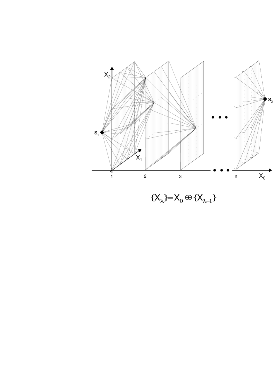
Figure 1: Diagrammatic illustration of the MDP method. In the multi–dimensional deformation space $\{X_{\lambda}\}$ we select the coordinate $\{X_{0}\}$ which is related in a linear way to the fission process. The points $s_{1}$ and $s_{2}$ correspond to entrance to the barrier and exit from the barrier, respectively. See text for details.

To find the least–action trajectory $L_{\rm min}$ between the turning point $s_{1}$ and $s_{2}$ we proceed as follows. First, we calculate the action–integrals from the entrance point under the barrier $s_{1}$ to all grid points in the nearest plane at $X_{0}=1$. In the next step we come to the plane at $X_{0}=2$ and from each grid point in this plane calculate the action–integrals to all grid points in the plane at $X_{0}=1$. The trajectories started from each grid point at $X_{0}=2$, passing through all grid points in the plane at $X_{0}=1$ and terminated in the point $s_{1}$, form a bunch of paths. From each such a bunch we choose the path with the minimal action–integral and bear it in mind. At the end of this step we have the least–action integrals along trajectories which connect the starting point $s_{1}$ with all grid points in the plane at $X_{0}=2$. Next, we repeat this procedure for all grid points at $X_{0}=3$ and again we obtain all the least–action–integrals along trajectories starting from point $s_{1}$ with ends at each grid point in the plane $X_{0}=3$. We repeat it until we reach the $n$–th plane, the last one before the exit point from the barrier $s_{2}$. Finally, we proceed to the last step of our method, where we calculate action–integrals between the exit point $s_{2}$ and all grid points situated on the last plane at $X_{0}=n$; the minimal one among them corresponds to the searched trajectory of the least–action–integral $L_{\rm min}$.

If we denote a number of grid points on each $X_{i}$ (i=1,2,…,$\lambda$-1) axis by $n_{i}$, then the whole number of trajectories examined in MDP method is equal to ($n_{1}\cdot{}n_{2}\cdot...\cdot{}n_{\lambda-1}$)ⁿ. Up to now, our calculations are carried out in a maximum of four–dimensional deformation space in view of an enormously large computational time (and disk space) required for preparing (and storing) input data with potential energy and $1/2\lambda(\lambda+1)$ components of symmetric inertia tensor for each of ($n_{1}\cdot{}n_{2}\cdot...\cdot{}n_{\lambda-1}$)$\cdot{}n$ grid points.

Calculations are performed in various four–, three– and two–dimensional deformation spaces spanned by selected shape parameters ($\beta_{\lambda}$, with $\lambda$=2,3,4,5,6 and 8) and two pairing degrees of freedom ($\Delta_{p},\Delta_{n}$). For $\beta$–shape parameters we used grids with steps $\Delta\beta_{2}$=$\Delta\beta_{3}$=0.05 and $\Delta\beta_{\lambda}$=0.04 for $\lambda$=4,5,6 and 8; in the case of pairing energy–gaps grids steps are equal 0.2 MeV. In our calculations a quadrupole deformation $\beta_{2}$ plays a role of the coordinate $X_{0}$ in Fig. 1.

3 RESULTS AND DISCUSSION

3.1 Optimal Multi–dimensional Deformation Space

The experimental values of the spontaneous fission half–lives of nine even–even Fm isotopes (N = 142, 144, …, 158) form approximately two sides of an acute–angled triangle with a vertex in N = 152. This strong nonlinear behaviour of $T^{SF}_{1/2}$ vs. neutron number N, due to an enhanced nuclear stability in the vicinity of deformed shell N=152, provides good opportunity for testing theoretical models.

To find the proper deformation space for description of the fission process we examined three different effects: the effect of the higher even–multipolarity shape parameters $\beta_{6}$ and $\beta_{8}$, the role of the reflection–asymmetry shape parameters $\beta_{3}$ and $\beta_{5}$, and the influence of the pairing degrees of freedom $\Delta_{p}$ and $\Delta_{n}$.

The following conclusions can be drawn from our previous dynamical analysis of $T^{SF}_{1/2}$ for Fm even–even isotopes, see Ref. [7, 8, 9]. In the case when the $\beta_{6}$ deformation parameter is added to our minimal two–dimensional space $\{\beta_{2},\beta_{4}\}$ we observed an increase of fission lifetimes by one to four orders of magnitude. The contribution of parameter $\beta_{8}$ to $T^{SF}_{1/2}$ is negligible.

The deformations with odd–multipolarity $\lambda$=3,5 do not change SF half–lives. The reason of this lies in the dynamical treatment of the fission process. The parameters $\beta_{3}$ and $\beta_{5}$ reduce the width of a static fission barrier, however the effective inertia $B_{eff}$, Eq. (17), along the corresponding static path is larger than along the dynamic one, where $\beta_{3}$ and $\beta_{5}$ are almost equal to zero. One can say, that the static path (corresponding to minimal potential energy) is “longer” than the dynamical one, for which $\beta_{3}$=$\beta_{5}$=0. The above conclusions are in agreement with those published in Ref. [26].

The pairing degrees of freedom $\Delta_{p}$ and $\Delta_{n}$ reduce SF half–lives for Fm isotopes with N$>$152 for about 3 orders of magnitude and considerably improve theoretical predictions of $T^{SF}_{1/2}$. This effect is due to strong dependence of the inertia tensor upon pairing energy–gap, as it was shown in Eq. (7).

Finally, we can conclude that the optimal deformation space for description of the fission half–lives of heavy nuclei is $\beta_{2},\beta_{4},\beta_{6},\Delta_{p}$ and $\Delta_{n}$.

Figure 2: The electric quadrupole moments of the even–even nuclei with atomic numbers Z=100–114, plotted as a function of the neutron number.

On account of computational limitations mentioned above, we can only perform calculations in a maximum of four–dimensional deformation space. So, we decided to define a correction to SF half–lives, which arises from pairing degrees of freedom, as the difference between $T^{SF}_{1/2}$ calculated in four–dimensional space $\{\beta_{2},\beta_{4},\Delta_{p},\Delta_{n}\}$ (when pairing degrees of freedom are treated as dynamical variables) and the one calculated in two–dimensional space $\{\beta_{2},\beta_{4}\}$ (where pairing energy–gaps are treated in the stationary way– i.e. by solving the BCS equations):

$$\delta T^{SF}_{1/2}(\Delta_{p},\Delta_{n})\equiv T^{SF}_{1/2}(\beta_{2},\beta_{4},\Delta_{p},\Delta_{n})-T^{SF}_{1/2}(\beta_{2},\beta_{4})\,.$$ (18)

Calculations of $T^{SF}_{1/2}$ in the space $\{\beta_{2},\beta_{4},\beta_{6},\Delta_{p},\Delta_{n}\}$ were approximated by the results obtained in three–dimensional space $\{\beta_{2},\beta_{4},\beta_{6}\}$ with the pairing correction $\delta T^{SF}_{1/2}(\Delta_{p},\Delta_{n})$.

3.2 Ground–state properties

Figure 3: The mean square radii of the even–even superheavy nuclei, plotted as a function of the neutron number.

In the present study of superheavy the even–even nuclei with atomic numbers Z=100-114 and neutron numbers N=142-180 are considered. First, we present the results related to ground–state (GS) properties. The GS properties were calculated in the equilibrium point found for a given nucleus by minimization of its potential energy with respect to $\beta_{2}$, $\beta_{4}$ and $\beta_{6}$ degrees of freedom.

In Fig. 2 we plot the electric quadrupole moments calculated with following formula

$$Q_{2}=\sqrt{\frac{16\pi}{5}}\sum_{\nu=p}\langle\,\nu\,|\,r^{2}Y_{20}\,|\,\nu\,\rangle\,v^{2}_{\nu}\,,$$ (19)

where $v^{2}_{\nu}$ is the BCS occupation factor corresponding to proton single–particle state $|\nu\rangle$ in the equilibrium point.

Almost all nuclei have distinct prolate deformations. And with an increase in the neutron number the $Q_{2}$ values show a regular decrease except at N=162–164, where a slight discontinuity in this behaviour can be seen for nuclei with atomic number Z$\geq$106.

The mean square charge radii (MSR), for the same region of nuclei, are plotted as a function of neutron number in Fig. 3. For calculations of MSR we use the usual formula

$$<r^{2}>=\frac{1}{\rm Z}\sum_{\nu=p}\langle\,\nu\,|\,r^{2}\,|\,\nu\,\rangle\,v^{2}_{\nu}+0.64\,{\rm fm^{2}}\,,$$ (20)

where the last term is due to finite range of proton charge distribution.

One observes a rather regular dependence of mean square radii on both neutron and proton number. However, as previously, close to N=162–164 one can see local maxima in MSR curves, particularly for nuclei with Z$\geq$106. This means that Coulomb repulsion energy for these nuclei is locally smaller, then they are more stable.

3.3 Spontaneous–fission versus alpha–decay

Figure 4: Contour map of the logarithm of the spontaneous–fission half-life (given in years) for nuclei shown in Fig. 2 calculated in $\{\beta_{2},\beta_{4},\beta_{6}\}$ deformation space and corrected by the effect of the pairing degrees of freedom, Eq. (18).

Figure 4 shows the results of the spontaneous–fission half–lives calculation, according to the MDP method, performed in $\{\beta_{2},\beta_{4},\beta_{6}\}$ deformation space with pairing correction $\delta T^{SF}_{1/2}(\Delta_{p},\Delta_{n})$, Eq. (18), for the nuclei shown in Fig. 2.

Two very specific effects can be observed on the contour map of $T^{SF}_{1/2}$ plotted as a function of neutron and proton numbers. One can see an enhancement in the SF half–life values at N=162 followed by a diminution at N=170.

The enhancement in nuclear stability near the deformed shell N=162 allows the appearance of a peninsula of deformed metastable superheavy nuclei. The local maximum of the $T^{SF}_{1/2}$ values is centered at the nucleus ${}^{268}_{106}{\rm Sg}_{162}$ (2.5 h).

In the vicinity of neutron number N=170 one observes the opposite behaviour. Here, the SF half–life values form a trench. This trench separates the peninsula of the deformed superheavy nuclei from an island of spherical superheavy elements around the doubly magic nucleus ${}^{298}114_{184}$. The local minimum is obtained for nucleus ${}^{272}_{102}{\rm No}_{170}$ (10 $\mu$s).

We found also that the $T^{SF}_{1/2}$ values of two heaviest nuclei (considered in the presented paper) ${}^{292}114_{178}$ and ${}^{294}114_{180}$ are comparable with those of the most stable Fm isotopes with neutron numbers N=152 and 154 ($\sim$ 100 yr).

In Fig. 5 we plot the alpha–decay half–lives (given in years) estimated by use of the Viola–Seaborg relationship with set of constants from Ref. [24]. The contour plot of the $T^{\alpha}_{1/2}$ forms a relatively regular surface descending steeply in the direction where the proton number tends to increase and the neutron number tends to decrease (upper–left–hand corner in the plot).

Figure 5: Contour plot of the logarithm of the alpha–decay half-life $T^{\alpha}_{1/2}$ (given in years) obtained from the Viola–Seaborg systematics. The alpha–decay energy was calculated with $\{\beta_{\lambda}\},\lambda=2,4,6$ deformation parameters.

The surface of the $T^{\alpha}_{1/2}$ values shows an evident protuberance at N=162, which demonstrates unambiguously the magicity of this neutron number. The shell effect at N=152 is very weak and disappears practically for nuclei with atomic number Z$>$104.

The results presented in Fig. 4 and 5 as well as conclusions drawn from them are generally similar to those recently published by other groups employing the macroscopic–microscopic method, Ref. [27, 28, 29, 30].

To compare the SF and $\alpha$-decay modes we show in Fig. 6 the logarithm of the total half–life $T^{SF+\alpha}_{1/2}$ resulting from both these modes. If we examine contour maps with $T^{SF+\alpha}_{1/2}$ and $T^{SF}_{1/2}$ we can notice some minor differences but the global behaviour of both these quantity stays unchanged.

The dark shadowed areas in Fig. 6 show the regions of nuclei in which the $\alpha$–decay mode predominates. The light shadowed area corresponds to the intermediate region of nuclei, where the probabilities of the SF and $\alpha$–decay processes are approximately equal (i.e. the region where the values of $T^{\alpha}_{1/2}$ and $T^{SF}_{1/2}$ differ up to one order of magnitude). The black solid curve inside this area connects nuclei for which probabilities of both considered modes are the same.

Thus, one can observe that the region of increased $\alpha$–decay activity separates two areas with predominating SF activity in a diagonal manner, in Fig. 6. It is worth noting that the upper area is almost inaccessible due to extremely short lifetimes ($\leq$ 1 $\mu$s).

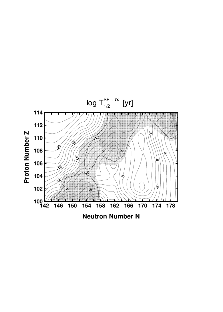
Figure 6: Logarithm of the total half-life $T^{SF+\alpha}_{1/2}$ resulting from SF (Fig. 4) and $\alpha$–decay (Fig. 5) modes. The dark shadowed areas show the regions of nuclei, where the $\alpha$–decay mode is a dominant one. The light shadowed area corresponds to the intermediate region, where the probabilities of SF and $\alpha$–decay modes are approximately equal.

The total half–life values (equal to $T^{\alpha}_{1/2}$) for two heaviest nuclei, considered in this paper, ${}^{292}114_{178}$ and ${}^{294}114_{180}$ are found larger than 1 yr. This is in agreement with results obtained recently in the fully selfconsistent microscopic nonrelativistic Hartrre–Fock–Bogoliubov approach, Ref. [31].

References

- [1] S. Hofmann et al.,Z. Phys. A350 (1995) 277.
- [2] S. Hofmann et al.,Z. Phys. A350 (1995) 281.
- [3] S. Hofmann et al.,Z. Phys. A354 (1996) 229.
- [4] Yu.A. Lazarev et al., Phys. Rev. Lett. 73 (1994) 624.
- [5] Yu.A. Lazarev et al., Phys. Rev. Lett. 75 (1995) 1903.
- [6] A. Türler, Proc. Inter. Workshop XXIV, Hirschegg 1996, ed. H. Feldmeier, J. Knoll and W. Nörenberg, GSI Darmstadt 1996, p. 29
- [7] Z. Łojewski and A. Staszczak, Acta. Phys. Pol. B27 (1996) 531.
- [8] A. Staszczak and Z. Łojewski, Proc. Inter. Workshop XXIV, Hirschegg 1996, ed. H. Feldmeier, J. Knoll and W. Nörenberg, GSI Darmstadt 1996, p. 98 (Report nucl–th/9603032).
- [9] Z. Łojewski and A. Staszczak, Annales Univ. MCS, Sectio AAA, L/LI (1995/1996) 137.
- [10] L.G. Moretto and R.B. Babinet, Phys. Lett. 49B (1974) 147.
- [11] A. Staszczak, A. Baran, K. Pomorski and K. Böning, Phys. Lett. 161B (1985) 227.
- [12] A. Staszczak, S. Piłat and K. Pomorski, Nucl. Phys. A504 (1989) 589.
- [13] S. Piłat and K. Pomorski and A. Staszczak, Proceed. Confer. Fifty Years with Nuclear Fission, vol.II, ed. J.W. Behrens, A.D. Carlson, American Nuclear Society, Gaithersburg 1989, p.637
- [14] J. Dudek, Report CRN/PHTH 91-19, Strasbourg 1991.
- [15] S.T. Belyaev, Mat. Fys. Medd. Dan. Vid. Selsk. 30 No 11 (1959); Nucl. Phys. 24 (1961) 322.
- [16] A. Góźdź, K. Pomorski, M. Brack and E. Werner, Nucl. Phys. A442 (1985) 26.
- [17] A. Sobiczewski, Z. Szymański, S. Wycech, S.G. Nilsson, J.R. Nix, C.F. Tsang, C. Gustafson, P. Möller and B. Nilsson, Nucl. Phys. A131 (1969) 67.
- [18] M. Brack, J. Damgaard, A.S. Jensen, H.C. Pauli, V.M. Strutinsky and C.Y. Wong, Rev. Mod. Phys. 44 (1972) 320.
- [19] V. M. Strutinsky, Nucl. Phys. A95 (1967) 420; Nucl. Phys. A122 (1968) 1.
- [20] H.J. Krappe, J.R. Nix and A.J. Sierk, Phys. Rev. C20 (1979) 992.
- [21] S. Ćwiok, J. Dudek, W. Nazarewicz, J. Skalski and T. Werner, Comput. Phys. Commun. 46 (1987) 379.
- [22] J. Dudek, A. Majhofer and J. Skalski, J. Phys. G6 (1980) 447.
- [23] V.E. Viola, Jr. and G.T. Seaborg, J. Inorg. Nucl. Chem. 28 (1966) 741.
- [24] A. Sobiczewski, Z. Patyk and S. Ćwiok, Phys. Lett. B224 (1989) 1.
- [25] A. Baran, K. Pomorski, A. Łukasiak and A. Sobiczewski, Nucl. Phys. A361 (1981) 83.
- [26] R. Smolańczuk, H.V. Klapdor–Kleingrothaus and A. Sobiczewski, Acta Phys. Pol. B24 (1993) 685.
- [27] R. Smolańczuk, J. Skalski and A. Sobiczewski, Phys. Rev. C52 (1995) 1871.
- [28] R. Smolańczuk, J. Skalski and A. Sobiczewski, Proc. Inter. Workshop XXIV, Hirschegg 1996, ed. H. Feldmeier, J. Knoll and W. Nörenberg, GSI Darmstadt 1996, p. 35.
- [29] P. Möller and J.R. Nix, J. Phys. G20 (1994) 1681
- [30] P. Möller, J.R. Nix and K.L. Kratz, At. Data. Nucl. Data Tables, to be published (Report nucl-th/9601043).
- [31] J.-F. Berger, L. Bitaud, J. Dechargé, M. Girod and S. Peru–Desenfants, Proc. Inter. Workshop XXIV, Hirschegg 1996, ed. H. Feldmeier, J. Knoll and W. Nörenberg, GSI Darmstadt 1996, p. 43.