Finite amplitude method for the RPA solution

Abstract

We propose a practical method to solve the random-phase approximation (RPA) in the self-consistent Hartree-Fock (HF) and density-functional theory. The method is based on numerical evaluation of the residual interactions utilizing finite amplitude of single-particle wave functions. The method only requires calculations of the single-particle Hamiltonian constructed with independent bra and ket states. Using the present method, the RPA calculation becomes possible with a little extension of a numerical code of the static HF calculation. We demonstrate usefulness and accuracy of the present method performing test calculations for isoscalar responses in deformed ²⁰Ne.

I Introduction

The mean-field theory with a density-dependent effective interaction has been an essential tool to understand nuclei. Thanks to the high performance computing, it is now becoming the most promising tool for quantitative description of nuclear structure in medium-to-heavy nuclei Bender et al. (2003); Lunney et al. (2003). The nuclear self-consistent mean-field theories are analogous to to the density-functional theory in condensed matter. A current major goal is constructing a universal energy-density functional, which is able to describe ground and excited states in nuclei and nuclear matter. This is also urgently needed for predicting and interpreting new data from the next generation of radioactive beam facilities.

In order to describe dynamical properties in nuclear response to external fields, the random-phase approximation (RPA) is a leading theory applicable to both low-lying states and giant resonances Ring and Schuck (1980). The RPA is a microscopic theory which can be obtained by linearizing the time-dependent Hartree-Fock (TDHF) equation, or equivalently, the time-dependent Kohn-Sham equation in the density-functional theory. The linearization produces a self-consistent residual interaction, $v=\delta^{2}E[\rho]/\delta\rho^{2}$, where $E$ and $\rho$ are the energy-density functional and the one-body density, respectively (Sec. II). The standard solution of the RPA is based on the matrix formulation of the RPA equation, which involves a large number of particle-hole matrix elements of the residual interaction, $v_{ph^{\prime},hp^{\prime}}$ and $v_{pp^{\prime},hh^{\prime}}$. Since the realistic nuclear energy functional is rather complicated, it is very tedious and difficult to calculate all the necessary matrix elements. It is, therefore, the purpose of the present paper to present an alternative method of solving the RPA equations, in which we deal with only the single-particle Hamiltonian, $h[\rho]$.

Although there are numerous works on the HF-plus-RPA calculations, because of the complexity of the residual interactions, it has been common in practice to neglect some parts of the residual interactions. The RPA calculations with full self-consistency are becoming a current trend in nuclear structure studies, however, they are essentially only for spherical nuclei at present Terasaki et al. (2005); Giambrone et al. (2003); Vretenar et al. (2001); Paar et al. (2003). The applications to deformed nuclei are very few, but have been done for the Skyrme energy functional using the three-dimensional mesh-space representation Nakatsukasa and Yabana (2002); Imagawa and Hashimoto (2003); Inakura et al. (2004); Nakatsukasa and Yabana (2005). See Sec. I in Ref. Terasaki et al. (2005) for a current status of these studies.

The basic idea of the present method is analogous to linear-response calculations in a time-dependent manner (real-time method) Nakatsukasa and Yabana (2002, 2005); Umar and Oberacher (2005). In the real-time method, the time evolution of a TDHF state involves only the action of the HF Hamiltonian, $h[\rho(t)]$, onto single-particle orbitals, $|{\psi_{i}(t)}\rangle$ ($i=1,\cdots,A$). Although the real-time method is very efficient for obtaining nuclear response in a wide energy range, its numerical instability caused by zero modes was a problem for the linear-response calculations Nakatsukasa and Yabana (2005). Zero-energy modes related to symmetry breaking in the HF state are easily excited, which often prevents the calculation of the time evolution for a long period. Therefore, it is desirable to develop a corresponding method in the frequency (energy) representation.

This paper is organized as follows. A new approach to the solution of the linear response equation, “finite amplitude method”, is presented in Sec. II. In Sec. III, using the Bonche-Koonin-Negele (BKN) interaction Bonche et al. (1976), we check the accuracy of solutions obtained with the present method. We also investigate the zero-energy components in calculated strength functions. Then, the conclusion is summarized in Sec. IV.

II Linear response theory

The RPA equation is known to be equivalent to the TDHF equation in the small-amplitude limit. We recapitulate how the RPA equation is derived from the small-amplitude TDHF equation, that will help explanation of our basic idea.

II.1 TDHF and linear response equation

The HF Hamiltonian, $h[\rho]=\delta E[\rho]/\delta\rho$, is a functional of one-body density matrix, $\rho$, which satisfies the condition, $\rho^{2}=\rho$, that the state is expressed by a single Slater determinant. The stationary condition is

$$[h[\rho],\rho]=0,$$ (1)

which defines the HF ground state density $\rho=\rho_{0}$. Hereafter, the static HF Hamiltonian is simply denoted as $h_{0}=h[\rho_{0}]$, and $\hbar=1$ is used. When a time-dependent external perturbation is present, the time evolution of the density, $\rho(t)$, follows the TDHF equation,

$$i\frac{d}{dt}\rho(t)=\big{[}\ h[\rho(t)]+V_{\rm ext}(t),\ \rho(t)\ \big{]}.$$ (2)

Using this $\rho(t)$, the expectation value of a one-body operator $F$ is obtained as $\langle F\rangle={\rm tr}\{F\rho(t)\}$. Provided that the perturbation is weak, we may linearize Eq. (2) with respect to $V_{\rm ext}(t)$ and $\delta\rho(t)$ defined by

$$\rho(t)=\rho_{0}+\delta\rho(t).$$ (3)

This leads to a time-dependent linear-response equation with an external field,

$$i\frac{d}{dt}\delta\rho(t)=[h_{0},\delta\rho(t)]+[V_{\rm ext}(t)+\delta h(t),\rho_{0}],$$ (4)

where $\delta h(t)$ is a residual field induced by density fluctuations,

$$\delta h(t)\equiv\frac{\delta h}{\delta\rho}\cdot\delta\rho(t)=\sum_{\mu\nu}\left.\frac{\partial h}{\partial\rho_{\mu\nu}}\right|_{\rho=\rho_{0}}\delta\rho_{\mu\nu}(t).$$ (5)

It should be noted that $\delta h(t)$ has a linear dependence on $\delta\rho(t)$. As we will see in Eq. (14), if we adopt the natural basis diagonalizing $h_{0}$, the summation can be restricted to the particle-hole ($\mu>A,\nu\leq A$) and hole-particle ($\mu\geq A,\nu<A$) components. Now, we decompose the time-dependent $\delta\rho(t)$ into those with fixed frequencies:

$$\delta\rho(t)=\sum_{\omega}\big{\{}\eta\delta\rho(\omega)e^{-i\omega t}+\eta^{*}\delta\rho^{\dagger}(\omega)e^{i\omega t}\big{\}}.$$ (6)

The external and induced fields are also expressed in the same way.

$$\delta h(t) = \sum_{\omega}\left\{\eta\delta h(\omega)e^{-i\omega t}+\eta^{*}\delta h^{\dagger}(\omega)e^{i\omega t}\right\},$$ (7)

$$V_{\rm ext}(t) = \sum_{\omega}\left\{\eta V_{\rm ext}(\omega)e^{-i\omega t}+\eta^{*}V_{\rm ext}^{\dagger}(\omega)e^{i\omega t}\right\}.$$ (8)

Here, we have introduced a small dimensionless parameter $\eta$. $\delta h(\omega)$ may be written as $\delta h(\omega)=\delta h/\delta\rho\cdot\delta\rho(\omega)$. Note that the transition density, the external field, and the induced field in the $\omega$-representation, $\delta\rho(\omega)$, $V_{\rm ext}(\omega)$, and $\delta h(\omega)$, are not necessarily hermitian. Substituting these into the linearized TDHF equation (4), we obtain the linear-response equation in the frequency representation,

$$\omega\ \delta\rho(\omega)=[h_{0},\delta\rho(\omega)]+[V_{\rm ext}(\omega)+\delta h(\omega),\rho_{0}].$$ (9)

This is the equation we want to solve in this paper.

When the frequency $\omega$ is equal to an RPA eigenfrequency $\omega_{n}$, there is a non-zero solution, $\delta\rho_{n}$, of Eq. (9) with $V_{\rm ext}=0$. These are called normal modes and are orthogonal to each other. The normalization is given by

$$\text{tr}\{[\delta\rho_{n}^{\dagger},\delta\rho_{n^{\prime}}]\rho_{0}\}=\langle{\Phi_{0}}|[\delta\rho_{n}^{\dagger},\delta\rho_{n^{\prime}}]|{\Phi_{0}}\rangle=\delta_{nn^{\prime}},$$ (10)

where $|{\Phi_{0}}\rangle$ indicates the HF ground state. From Eq. (10), it is obvious that, in order to normalize the transition density $\delta\rho_{n}$, it must be non-hermitian. When $\omega=\omega_{n}$, the nucleus is truly excited by $V_{\rm ext}(\omega)$, and we cannot determine the magnitude of $\delta\rho(\omega_{n})$ because $\delta\rho(t)$ increases in time. If $\delta\rho(\omega_{n})$ is a solution of Eq. (9), $\delta\rho(\omega_{n})+c\delta\rho_{n}$ with an arbitrary constant $c$ is a solution too.

So far, the linear-response equation has been expressed in terms of the one-body density operators. The density-matrix formulation is simple and easy to manipulate, however, in practical calculations, it is convenient to introduce single-particle (Kohn-Sham) orbitals. For systems with $A$ particles, the TDHF describes the one-body density using $A$ single-particle orbitals, $|{\psi_{i}(t)}\rangle$,

$$\rho(t)=\sum_{i=1}^{A}|{\psi_{i}(t)}\rangle\langle{\psi_{i}(t)}|,\quad\quad\quad\rho_{0}=\sum_{i=1}^{A}|{\phi_{i}}\rangle\langle{\phi_{i}}|.$$ (11)

It is an advantage of the TDHF, that the time evolution is described by occupied orbitals only, $\{|{\psi_{i}}\rangle\}$ with $i=1,\cdots,A$. The static orbitals are normally chosen as eigenstates of the HF Hamiltonian,

$$h_{0}|{\phi_{\mu}}\rangle=\epsilon_{\mu}|{\phi_{\mu}}\rangle,$$ (12)

which can be divided into two categories; occupied (hole) orbitals, $\{\phi_{i}\}$ ($i=1,\cdots,A$), for which we use indexes $i,j,\cdots$, and unoccupied (particle) orbitals, $\{\phi_{m}\}$ ($m=A+1,\cdots$), for which we use indexes $m,n,\cdots$. In the linear approximation, we have

$$\delta\rho(t)=\sum_{i}\big{\{}|{\phi_{i}}\rangle\langle{\delta\psi_{i}(t)}|+|{\delta\psi_{i}(t)}\rangle\langle{\phi_{i}}|\big{\}},$$ (13)

where $|{\psi_{i}(t)}\rangle=(|{\phi_{i}}\rangle+|{\delta\psi_{i}(t)}\rangle)e^{-i\epsilon_{i}t}$ and it is linearized with respect to $|{\delta\psi_{i}(t)}\rangle$. The condition, $\rho(t)^{2}=\rho(t)$, leads to

$$\delta\rho_{ij}=\delta\rho_{mn}=0,\quad\quad i,j\leq A,\quad m,n>A,$$ (14)

$$\langle\phi_{j}|\delta\psi_{i}\rangle+\langle\delta\psi_{j}|\phi_{i}\rangle=0.$$ (15)

The second equation is nothing but the orthonormalization condition for single-particle orbitals, $\{|{\psi_{i}(t)}\rangle\}$ ($i=1,\cdots,A$).

Transforming $\delta\rho(t)$ into $\delta\rho(\omega)$ in Eq. (6), we must make ket and bra states independent, because $\delta\rho(\omega)$ is not hermitian. This is related to the fact that the RPA equation is described by forward and backward amplitudes, $X(\omega)$ and $Y(\omega)$.

$$\delta\rho(\omega)=\sum_{i}\big{\{}|{X_{i}(\omega)}\rangle\langle{\phi_{i}}|+|{\phi_{i}}\rangle\langle{Y_{i}(\omega)}|\big{\}}.$$ (16)

This is equivalent to the Fourier decomposition of the time-dependent single-particle orbitals,

$$|{\delta\psi_{i}(t)}\rangle=\sum_{\omega}\big{\{}\eta|{X_{i}(\omega)}\rangle e^{-i\omega t}+\eta^{*}|{Y_{i}(\omega)}\rangle e^{i\omega t}\big{\}}.$$ (17)

Since only the particle-hole matrix elements of $\delta\rho(\omega)$ are non-zero, seen in Eq. (14), we can assume that the amplitudes, $|{X_{i}(\omega)}\rangle$ and $|{Y_{i}(\omega)}\rangle$, can be expanded in the particle orbitals only;

$$|{X_{i}(\omega)}\rangle=\sum_{m>A}|{\phi_{m}}\rangle X_{mi}(\omega),\quad\quad|{Y_{i}(\omega)}\rangle=\sum_{m>A}|{\phi_{m}}\rangle Y_{mi}^{*}(\omega).$$ (18)

If we take particle-hole and hole-particle matrix elements of Eq. (9), we can derive the well-known RPA equation in the matrix form;

$$\left\{\begin{pmatrix}A&B\\ B^{*}&A^{*}\end{pmatrix}-\omega\begin{pmatrix}1&0\\ 0&-1\end{pmatrix}\right\}\begin{pmatrix}X_{nj}(\omega)\\ Y_{nj}(\omega)\end{pmatrix}=-\begin{pmatrix}f(\omega)\\ g(\omega)\end{pmatrix}.$$ (19)

Here, the matrices, $A$ and $B$, and the vectors, $f$ and $g$, are defined by

$$A_{mi,nj} \equiv (\epsilon_{m}-\epsilon_{i})\delta_{mn}\delta_{ij}+\langle{\phi_{m}}|\left.\frac{\partial h}{\partial\rho_{nj}}\right|_{\rho=\rho_{0}}|{\phi_{i}}\rangle,$$ (20)

$$B_{mi,nj} \equiv \langle{\phi_{m}}|\left.\frac{\partial h}{\partial\rho_{jn}}\right|_{\rho=\rho_{0}}|{\phi_{i}}\rangle,$$ (21)

$$f_{mi}(\omega) \equiv \langle{\phi_{m}}|V_{\rm ext}(\omega)|{\phi_{i}}\rangle,\quad g_{mi}(\omega)\equiv\langle{\phi_{i}}|V_{\rm ext}(\omega)|{\phi_{m}}\rangle.$$ (22)

For the normal modes that are homogeneous solutions of Eq. (19), the orthogonality and normalization are expressed as

$$\sum_{m,i}\left\{X_{mi}^{(n)*}X_{mi}^{(n^{\prime})}-Y_{mi}^{(n)*}Y_{mi}^{(n^{\prime})}\right\}=\delta_{nn^{\prime}},$$ (23)

which is equivalent to Eq. (10). This is a standard matrix formulation of the RPA equation. In practical applications, the most tedious part is calculation of matrix elements of the residual interactions in $A_{mi,nj}$ and $B_{mi,nj}$. In Ref. Muta et al. (2002), a numerical method to solve the RPA equation in the coordinate space is proposed, and the similar approaches are used in realistic applications using the Skyrme interaction Imagawa and Hashimoto (2003); Inakura et al. (2004). In those works, one does not need to calculate the particle orbitals, however, the residual interaction must be evaluated in the coordinate-space representation. In Sec. II.2, we propose an alternative, even simpler approach to a solution of the linear-response equation (9). The method does not require explicit evaluation of the residual interaction, $\delta h/\delta\rho$.

II.2 Finite amplitude method

Multiplying both sides of Eq. (9) with a ket of hole states $|{\phi_{i}}\rangle$, we have

$$\omega|{X_{i}(\omega)}\rangle=(h_{0}-\epsilon_{i})|{X_{i}(\omega)}\rangle+\hat{Q}\left\{V_{\rm ext}(\omega)+\delta h(\omega)\right\}|{\phi_{i}}\rangle,$$ (24)

where $\hat{Q}$ is a projection operator onto the particle space, $\hat{Q}=1-\sum_{j}|{\phi_{j}}\rangle\langle{\phi_{j}}|$. Another equation can be derived by multiplying a bra state $\langle{\phi_{i}}|$ with Eq. (9).

$$\omega\langle{Y_{i}(\omega)}|=-\langle{Y_{i}(\omega)}|(h_{0}-\epsilon_{i})-\langle{\phi_{i}}|\left\{V_{\rm ext}(\omega)+\delta h(\omega)\right\}\hat{Q}.$$ (25)

These are formally equivalent to the RPA equation in the matrix form of Eq. (19).

The essential idea of our new numerical approach is as follow: Equations (24) and (25) require operations of the HF Hamiltonian in the ground state, $h_{0}$, and the induced fields, $\delta h(\omega)$ and $\delta h^{\dagger}(\omega)$. Since $h_{0}$ is obtained by the static HF calculation, a new ingredient for the RPA calculation is the latter two. The conventional approach is to expand $\delta h(\omega)$ in the linear order as Eq. (5), then to solve the RPA equation in a matrix form. In this paper, instead of performing the explicit expansion, we resort to the numerical linearization. Now, let us explain how to achieve it.

The time-dependent self-consistent Hamiltonian, $h(t)$, is a functional of one-body density that is represented by occupied $A$ single-particle states; $h[\rho(t)]=h[\psi(t)]$. In the linear approximation,

$$h[\rho_{0}+\delta\rho(t)]=h[\phi+\delta\psi(t)]=h_{0}+\delta h(t),$$ (26)

the induced field can be written as $\delta h(t)=h[\phi+\delta\psi(t)]-h_{0}$. In the frequency representation, the story becomes slightly more complicated, because $\delta h(\omega)$ and $\delta h^{\dagger}(\omega)$, are no longer hermitian. In this case, we should regard $h[\rho]$ as a functional of $2A$ single-particle states (independent bra and ket), $\langle{\psi^{\prime}_{i}}|$ and $|{\psi_{i}}\rangle$, $i=1,\cdots,A$. We denote it as $h\big{[}\langle{\psi^{\prime}}|,|{\psi}\rangle\big{]}$. Using Eq. (16), we may write the non-hermitian density as

$$\rho_{0}+\eta\delta\rho(\omega) = \sum_{i}\left\{|{\phi_{i}}\rangle\langle{\phi_{i}}|+\eta|{X_{i}(\omega)}\rangle\langle{\phi_{i}}|+\eta|{\phi_{i}}\rangle\langle{Y_{i}(\omega)}|\right\}$$ (27)

$$= \sum_{i}\left\{|{\phi_{i}}\rangle+\eta|{X_{i}(\omega)}\rangle\right\}\left\{\langle{\phi_{i}}|+\eta\langle{Y_{i}(\omega)}|\right\}.$$ (28)

In the last equation, we assume the linear approximation with respect to $\eta$. The fact that $\delta h(\omega)$ is proportional to $\delta\rho(\omega)$ and $\delta h^{\dagger}(\omega)$ proportional to $\delta\rho^{\dagger}(\omega)$ leads to

$$h_{0}+\eta\ \delta h(\omega) = h[\rho_{0}+\eta\delta\rho(\omega)]=h\big{[}\langle{\phi}|+\eta\langle{Y(\omega)}|,|{\phi}\rangle+\eta|{X(\omega)}\rangle\big{]},$$ (29)

$$h_{0}+\eta\ \delta h^{\dagger}(\omega) = h[\rho_{0}+\eta\delta\rho^{\dagger}(\omega)]=h\big{[}\langle{\phi}|+\eta\langle{X(\omega)}|,|{\phi}\rangle+\eta|{Y(\omega)}\rangle\big{]},$$ (30)

up to the first order in a small parameter $\eta$. In other words, the induced fields may be calculated using the finite difference with respect to $\eta$;

$$\delta h(\omega)=\frac{1}{\eta}\left(h\big{[}\langle{\psi^{\prime}}|,|{\psi}\rangle\big{]}-h[\langle{\phi}|,|{\phi}\rangle\big{]}\right),$$ (31)

where $\langle{\psi^{\prime}_{i}}|=\langle{\phi_{i}}|+\eta\langle{Y_{i}(\omega)}|$ and $|{\psi_{i}}\rangle=|{\phi_{i}}\rangle+\eta|{X_{i}(\omega)}\rangle$. Its hermitian conjugate, $\delta h^{\dagger}(\omega)$, may be expressed as the same equation (31), but with $\langle{\psi^{\prime}_{i}}|=\langle{\phi_{i}}|+\eta\langle{X_{i}(\omega)}|$ and $|{\psi_{i}}\rangle=|{\phi_{i}}\rangle+\eta|{Y_{i}(\omega)}\rangle$.

Using these numerical differentiation, the r.h.s. of the RPA equations, (24) and (25), can be easily calculated by action of the HF Hamiltonian, $h\big{[}\langle{\psi^{\prime}}|,|{\psi}\rangle\big{]}$, on the single-particle orbitals, $|{\phi_{i}}\rangle$. For the first sight, Eqs. (24) and (25) do not look like linear equations. However, since $\delta h(\omega)$ linearly depends on $|{X_{i}(\omega)}\rangle$ and $\langle{Y_{i}(\omega)}|$, they are inhomogeneous linear equations with respect to $|{X_{i}(\omega)}\rangle$ and $\langle{Y_{i}(\omega)}|$. It is obvious in a sense that they are equivalent to the matrix form of Eq. (19), Therefore, we can employ a well-established iterative method for their solutions. If the linear equation is described by a hermitian matrix, the conjugate gradient method (CGM) is one of the most powerful method. However, in general, we may take the frequency $\omega$ complex, then, the RPA matrix becomes non-hermitian. Then, we should use another kind of iterative solver, for instance, the bi-conjugate gradient method (Bi-CGM). A typical numerical procedure is as follows: (i) Fix the frequency $\omega$ that can be complex, and assume initial vectors ($n=0$), $|{X_{i}^{(n)}(\omega)}\rangle$ and $\langle{Y_{i}^{(n)}(\omega)}|$. (ii) Update the vectors, $|{X_{i}^{(n+1)}(\omega)}\rangle$ and $\langle{Y_{i}^{(n+1)}(\omega)}|$, using the algorithm of an iterative method, such as CGM and Bi-CGM. (iii) Calculate the residual of Eqs. (24) and (25). If its magnitude is smaller than a given accuracy, stop the iteration. Otherwise, go back to the step (ii) with $n\rightarrow n+1$.

The most advantageous feature of the present approach is that it only requires operations of the HF Hamiltonian, $h\big{[}\langle{\psi^{\prime}}|,|{\psi}\rangle\big{]}$. These are usually included in computational programs of the static HF calculations. Only extra effort necessary is to estimate the HF Hamiltonian with different bra and ket single-particle states, $\langle{\psi_{i}^{\prime}}|$ and $|{\psi_{i}}\rangle$. Therefore, a minor modification of the static HF computer code will provide a numerical solution of the RPA equations. Hereafter, we call this numerical approach “finite amplitude method”. Apparently, the present method is also applicable to the RPA eigenvalue problems with a trivial modification.

II.3 Transition strength in the linear response

In this subsection, we present how to calculate transition strength using solutions of Eqs. (24) and (25). Assuming that the system is at its ground state $|{\Phi_{0}}\rangle$ with energy $E_{0}=0$ at $t=-\infty$, and that the external field $V_{\rm ext}(t)$ is adiabatically switched on ($\omega\rightarrow\omega\pm i\epsilon$ in Eq. (8)), the state at time $t$ will be

$$|{\Psi(t)}\rangle=|{\Phi_{0}}\rangle-i\sum_{n}e^{-iE_{n}t}\int_{-\infty}^{t}dt^{\prime}e^{iE_{n}t^{\prime}}|{\Phi_{n}}\rangle\langle{\Phi_{n}}|V_{\rm ext}(t^{\prime})|{\Phi_{0}}\rangle.$$ (32)

in the first-order approximation with respect to $V_{\rm ext}$. Here, $|{\Phi_{n}}\rangle$ and $E_{n}$ are the $n$-th excited state and its excitation energy, respectively. Especially, if the external field has a fixed frequency $\omega>0$, $V_{\rm ext}(t)=\eta Fe^{-i\omega t}+\eta^{*}F^{\dagger}e^{i\omega t}$, this is written as

$$|{\Psi(t)}\rangle=|{\Phi_{0}}\rangle-i\sum_{n}|{\Phi_{n}}\rangle\left(\frac{\eta\langle{\Phi_{n}}|F|{\Phi_{0}}\rangle}{\omega-E_{n}+i\epsilon}e^{-i\omega t}-\frac{\eta^{*}\langle{\Phi_{n}}|F^{\dagger}|{\Phi_{0}}\rangle}{\omega+E_{n}-i\epsilon}e^{i\omega t}\right),$$ (33)

where $F$ is an arbitrary one-body operator, Then, the expectation value of $F^{\dagger}$ at time $t$ is

$$\langle{\Psi(t)}|F^{\dagger}|{\Psi(t)}\rangle \equiv \langle{\Phi_{0}}|F^{\dagger}|{\Phi_{0}}\rangle+\eta S(F;\omega)e^{-i\omega t}+\cdots,$$ (34)

$$S(F;\omega) = \sum_{n}\left(\frac{|\langle{\Phi_{n}}|F|{\Phi_{0}}\rangle|^{2}}{\omega-E_{n}+i\epsilon}-\frac{|\langle{\Phi_{n}}|F^{\dagger}|{\Phi_{0}}\rangle|^{2}}{\omega+E_{n}-i\epsilon}\right).$$ (35)

Taking the limit of $\epsilon\rightarrow 0$, we have the transition strength,

$$\frac{dB(\omega;F)}{d\omega}\equiv\sum_{n}|\langle{\Phi_{n}}|F|{\Phi_{0}}\rangle|^{2}\delta(\omega-E_{n})=-\frac{1}{\pi}\mbox{Im}S(F;\omega).$$ (36)

Comparing Eq. (34) with the expectation value in the TDHF state,

$$\mbox{tr}\big{\{}F^{\dagger}\rho(t)\big{\}}=\mbox{tr}\big{\{}F^{\dagger}\rho_{0}\big{\}}+\mbox{tr}\big{\{}F^{\dagger}\delta\rho(\omega)\big{\}}e^{-i\omega t}+\cdots.$$ (37)

$S(F:\omega)$ in the RPA is written as

$$S_{\rm RPA}(F;\omega) = \mbox{tr}\big{\{}F^{\dagger}\delta\rho(\omega)\big{\}}=i\mbox{tr}\big{\{}[\delta\rho_{F}^{\dagger},\delta\rho(\omega)]\big{\}}$$ (38)

$$= \sum_{i}\left(\langle{\phi_{i}}|F^{\dagger}|{X_{i}(\omega)}\rangle+\langle{Y_{i}(\omega)}|F^{\dagger}|{\phi_{i}}\rangle\right).$$ (39)

Here, $\delta\rho_{F}$ is defined by $\delta\rho_{F}\equiv i[F,\rho_{0}]$.

II.4 Separation of Nambu-Goldstone modes

The RPA theory is known to have a property that the zero-energy modes are exactly decoupled from physical (intrinsic) modes of excitation. Since the zero modes are associated with the symmetry breaking in the HF ground state, it is also called “Nambu-Goldstone modes” (NG modes). When $P$ is a hermitian symmetry operator of the Hamiltonian, $[H,P]=0$, then, the transformed ground-state density, $\tilde{\rho}_{0}=e^{i\alpha P}\rho_{0}e^{-i\alpha P}$, also satisfies the HF equation (1). Expanding the equation up to the first order in $\alpha$, we have

$$[h_{0},\delta\tilde{\rho}]+[\delta\tilde{h},\rho_{0}]=0,$$ (40)

where

$$\delta\tilde{\rho}\equiv\tilde{\rho}_{0}-\rho_{0}=i\alpha[P,\rho_{0}],\quad\quad\delta\tilde{h}\equiv h[\tilde{\rho}_{0}]-h_{0}=\frac{\delta h}{\delta\rho}\cdot\delta\tilde{\rho}.$$ (41)

This indicates that $\delta\tilde{\rho}$ is an RPA eigenmode corresponding to $\omega=0$. $\delta\rho$ generated by the operator $R$ conjugate to $P$ ($[R,P]=i$) can be defined in a similar manner. For instance, the translational symmetry is expressed by the total momentum as $P$ and the center-of-mass coordinate as $R$. We denote these transition densities associated with the NG mode as

$$\delta\rho_{P} \equiv i[P,\rho_{0}]=\frac{1}{\alpha}\delta\tilde{\rho}=\sum_{i}\left(|{\bar{P}_{i}}\rangle\langle{\phi_{i}}|+|{\phi_{i}}\rangle\langle{\bar{P}_{i}}|\right),$$ (42)

$$\delta\rho_{R} \equiv i[R,\rho_{0}]=\sum_{i}\left(|{\bar{R}_{i}}\rangle\langle{\phi_{i}}|+|{\phi_{i}}\rangle\langle{\bar{R}_{i}}|\right),$$ (43)

where we have defined $|{\bar{P}_{i}}\rangle\equiv iP|{\phi_{i}}\rangle$ and $|{\bar{R}_{i}}\rangle\equiv iR|{\phi_{i}}\rangle$. Provided that $P$ and $R$ are hermitian, $\delta\rho_{P}$ and $\delta\rho_{Q}$ are also hermitian. Therefore, we cannot normalize them in terms of the normalization condition of Eq. (10). These modes are automatically orthogonal to other normal modes with $\omega\neq 0$. If we solve the RPA equation fully self-consistently, the NG modes should be clearly separated from other modes. However, in practice, we often encounter a mixture of spurious components in physical excitations. For instance, the coordinate-space is discretized in mesh to represent wave functions in Sec. III, which violates the exact translational and rotational symmetries. We also use a smoothing parameter $\Gamma$ to make the frequency complex, then, low-lying excited states are embedded in a large tail of the NG-mode strength ($\delta\rho(\omega)\rightarrow\infty$ for $\omega\rightarrow 0$ ). Here, we present a prescription to remove the strength associated with the NG mode.

Let us assume that there is a mixture of NG modes in a calculated transition density, $\delta\rho_{\rm cal}(\omega)$.

$$\delta\rho_{\rm cal}(\omega)=\delta\rho_{\rm phy}(\omega)+\lambda_{P}\delta\rho_{P}+\lambda_{R}\delta\rho_{R},$$ (44)

where “physical” transition density, $\delta\rho_{\rm phy}(\omega)$, is free from the NG modes. Here, we assume there is a single NG mode, for simplicity. It is straightforward to extend the present prescription to the one for more than one NG modes. Since $\delta\rho_{\rm phy}$ should be orthogonal to the NG modes, $\delta\rho_{\rm phy}$ should satisfy

$$\langle{\Phi_{0}}|[\delta\rho_{P},\delta\rho_{\rm phy}(\omega)]|{\Phi_{0}}\rangle=\langle{\Phi_{0}}|[\delta\rho_{R},\delta\rho_{\rm phy}(\omega)]|{\Phi_{0}}\rangle=0.$$ (45)

Utilizing the canonicity condition, $[R,P]=i$, the orthogonality condition, Eq. (45), determines the coefficients, $\lambda_{P(R)}$, as

$$\lambda_{P} = -i\sum_{i}\left(\langle\bar{R}_{i}|X_{i}(\omega)\rangle-\langle Y_{i}(\omega)|\bar{R}_{i}\rangle\right),$$ (46)

$$\lambda_{R} = i\sum_{i}\left(\langle\bar{P}_{i}|X_{i}(\omega)\rangle-\langle Y_{i}(\omega)|\bar{P}_{i}\rangle\right).$$ (47)

Substituting these into Eq. (44), we may extract $\delta\rho_{\rm phy}(\omega)$ from the “contaminated” transition density $\delta\rho_{\rm cal}(\omega)$.

III Numerical Applications

III.1 Coordinate-space representation

In case of zero-range effective interactions, such as Skyrme interactions, the HF Hamiltonian, $h({\mathbf{r}})=h[\rho({\mathbf{r}})]$, is a functional of local one-body densities. Then, it is convenient to adopt the coordinate-space representation. In the followings, we assume ${\mathbf{r}}$ involves the spin and isospin indexes, if necessary. The RPA equations, (24) and (25), for a complex frequency $\omega$ can be written in the ${\mathbf{r}}$-representation as

$$\big{(}h_{0}({\mathbf{r}})-\epsilon_{i}-\omega\big{)}X_{i}({\mathbf{r}},\omega)+\delta h({\mathbf{r}},\omega)\phi_{i}({\mathbf{r}}) = -V_{\rm ext}({\mathbf{r}},\omega)\phi_{i}({\mathbf{r}}),$$ (48)

$$\left\{\big{(}h_{0}({\mathbf{r}})-\epsilon_{i}+\omega^{*}\big{)}Y_{i}({\mathbf{r}},\omega)+\delta h^{\dagger}({\mathbf{r}},\omega)\phi_{i}({\mathbf{r}})\right\}^{*} = -\left\{V_{\rm ext}^{\dagger}({\mathbf{r}},\omega)\phi_{i}({\mathbf{r}})\right\}^{*}.$$ (49)

Here, for simplicity, we omit the projection operator, $\hat{Q}$, on both sides of these equations. In the finite amplitude method, the operation of $\delta h({\mathbf{r}},\omega)$ is calculated by

$$\delta h({\mathbf{r}},\omega)\phi_{i}({\mathbf{r}})=\frac{1}{\eta}\left(h\big{[}\psi^{\prime*},\psi\big{]}({\mathbf{r}})\phi_{i}({\mathbf{r}})-\epsilon_{i}\phi_{i}({\mathbf{r}})\right),$$ (50)

with $\psi^{\prime*}_{i}({\mathbf{r}})=\phi_{i}^{*}({\mathbf{r}})+\eta Y_{i}^{*}(\omega,{\mathbf{r}})$ and $\psi_{i}({\mathbf{r}})=\phi_{i}({\mathbf{r}})+\eta X_{i}({\mathbf{r}},\omega)$. Exchanging the forward and backward amplitudes in $\psi_{i}({\mathbf{r}})$ and $\psi^{\prime}_{i}({\mathbf{r}})$, we may calculate $\delta h^{\dagger}({\mathbf{r}},\omega)\phi_{i}({\mathbf{r}})$ in the same way.

Adopting the fixed-$\omega$ local external field

$$V_{\rm ext}({\mathbf{r}},\omega^{\prime})=\delta_{\omega\omega^{\prime}}F({\mathbf{r}}),$$ (51)

the transition strength can be obtained from the calculated forward and backward amplitudes,

$$\frac{dB(\omega;F)}{d\omega} \equiv \sum_{n}|\langle{n}|F|{0}\rangle|^{2}\delta(\omega-E_{n}),$$ (52)

$$= -\frac{1}{\pi}\mbox{Im}\sum_{i}\int d{\mathbf{r}}\left\{\phi_{i}^{*}({\mathbf{r}})F^{\dagger}({\mathbf{r}})X_{i}({\mathbf{r}},\omega)+Y_{i}^{*}({\mathbf{r}},\omega)F^{\dagger}({\mathbf{r}})\phi_{i}({\mathbf{r}})\right\}.$$ (53)

We apply the present method to the BKN interaction which contains two-body (zero- and finite-range) and three-body interactions. For this schematic interaction, the spin-isospin degeneracy is assumed all the time and the Coulomb potential acts on all orbitals with a charge $e/2$ Bonche et al. (1976). The HF one-body Hamiltonian in the coordinate-space representation is given by

$$h[\rho]=\frac{1}{2m}\nabla^{2}+\frac{3}{4}t_{0}\rho({\mathbf{r}})+\frac{3}{16}\rho^{2}({\mathbf{r}})+W_{Y}[\rho]({\mathbf{r}})+W_{C}[\rho]({\mathbf{r}}),$$ (54)

where the Yukawa potential, $W_{Y}$, and Coulomb potential, $W_{C}$, consist of their direct terms only. For the finite amplitude approach, it is convenient to rewrite Eq. (54) as

$$h[\psi^{\prime*},\psi]({\mathbf{r}}) = \frac{1}{2m}\nabla^{2}+\frac{3}{4}t_{0}\sum_{i=1}^{A/4}4\psi_{i}({\mathbf{r}})\psi_{i}^{\prime*}({\mathbf{r}})+\frac{3}{16}\left\{\sum_{i=1}^{A/4}4\psi_{i}({\mathbf{r}})\psi_{i}^{\prime*}({\mathbf{r}})\right\}^{2}$$ (55)

$$\quad\quad+\int d{\mathbf{r}}^{\prime}v({\mathbf{r}}-{\mathbf{r}}^{\prime})\sum_{i=1}^{A/4}4\psi_{i}({\mathbf{r}}^{\prime})\psi^{\prime*}_{i}({\mathbf{r}}^{\prime}),$$

where $v({\mathbf{r}})$ is a sum of the Yukawa and the Coulomb potential,

$$v({\mathbf{r}})\equiv V_{0}a\frac{e^{-r/a}}{r}+\frac{(e/2)^{2}}{|{\mathbf{r}}|}.$$ (56)

We adopt the parameter values from Ref. Bonche et al. (1976).

III.2 Numerical details

We use the three-dimensional (3D) coordinate-space representation for solving the RPA equations. The model space is a sphere of radius of 10 fm, discretized in square mesh of $\Delta x=\Delta y=\Delta z=0.8$ fm. The number of grid points in the sphere is 8217. The differentiation is approximated by the nine-point formula. The frequency $\omega$ is varied from zero to 40 MeV with a spacing of $\Delta\omega=200$ keV (201 points). A small imaginary part is added to $\omega$: $\omega\rightarrow\omega+i\Gamma/2$ with $\Gamma=500$ keV. In numerical calculations, we use real variables with double precision ($8$ bytes) and complex variables of $8\times 2$ bytes. In Eq. (50), we choose the parameter $\eta$ in $\psi_{i}({\mathbf{r}})=\phi_{i}({\mathbf{r}})+\eta X_{i}({\mathbf{r}})$ and $\psi_{i}^{\prime*}({\mathbf{r}})=\phi_{i}^{*}({\mathbf{r}})+\eta Y_{i}^{*}({\mathbf{r}})$, as follows:

$$\eta=\frac{10^{-5}}{\max\{N(X),N(Y)\}},\quad\quad N(\delta\psi)\equiv\frac{1}{A}\sqrt{\sum_{i}\langle\delta\psi_{i}|\delta\psi_{i}\rangle,\}}.$$ (57)

In order to obtain the forward and backward amplitudes at a frequency $\omega$, we adopt the Bi-CGM as an iterative solver for Eqs. (48) and (49), starting from the initial values of $X_{i}({\mathbf{r}})=Y_{i}^{*}({\mathbf{r}})=0$. We set the convergence condition that the ratio of the remaining difference to the r.h.s. of Eqs. (48) and (49) is less than $10^{-5}$. The number of iteration necessary to reach the convergence depends on the choice of the external field $V_{\rm ext}(\omega)$, the frequency $\omega$, the smoothing parameter $\Gamma$, and residual interactions included in the calculation. The convergence is relatively slow for an external field coupled to the NG modes. A larger number of iteration is required for a larger $\omega$ value. Typically, the calculation reaches the convergence in 10 to 100 iterations for $\omega<10$ MeV, but it requires more than 500 iterations for $\omega>30$ MeV. The number also depends on the smoothing parameter $\Gamma$. Roughly speaking, larger number of iteration seems to be required for smaller $\Gamma$. If we neglect the residual Coulomb and Yukawa interactions of finite range, the convergence becomes much faster. We solve the differential equations to obtain the Coulomb and Yukawa potentials using the CGM Flocard et al. (1978).

$$\nabla^{2}V_{C}=-2\pi e^{2}\rho({\mathbf{r}}),\quad\quad\left(\nabla^{2}-\frac{1}{a^{2}}\right)V_{Y}=-4\pi V_{0}a\rho({\mathbf{r}}).$$ (58)

It turns out to be important to solve these equations with high accuracy. We set the convergence condition that the ratio of the remaining difference to the r.h.s. of Eq. (58) is less than $10^{-23}$. Since the convergence of the CGM is very fast, this is not a problem.

III.3 Results

In this section, we show calculated response for isoscalar (IS) modes of compressional dipole, quadrupole and octupole for ²⁰Ne. The main purpose of the calculation is to test capability of the present numerical approach, the finite amplitude method. The ²⁰Ne nucleus has a prolate shape with a quadrupole deformation $\beta\approx 0.4$ in the HF ground state. Identifying the symmetry axis with $z$-axis, we use external fields with a fixed frequency, $V_{\rm ext}({\mathbf{r}},\omega)=Q_{\lambda K}({\mathbf{r}})$,

$$Q_{\lambda K}({\mathbf{r}})=\begin{cases}r^{3}Y_{10}(\hat{\mathbf{r}}),\quad r^{3}Y_{11}(\hat{\mathbf{r}}),&\text{for IS dipole, }\lambda=1\\ r^{2}Y_{20}(\hat{\mathbf{r}}),\quad r^{2}Y_{21}(\hat{\mathbf{r}}),\quad r^{2}Y_{22}(\hat{\mathbf{r}}),&\text{for IS quadrupole, }\lambda=2\\ r^{3}Y_{30}(\hat{\mathbf{r}}),\quad r^{3}Y_{31}(\hat{\mathbf{r}}),\quad r^{3}Y_{32}(\hat{\mathbf{r}}),\quad r^{3}Y_{33}(\hat{\mathbf{r}}),&\text{for IS octupole, }\lambda=3.\end{cases}$$ (59)

Then, the strength distribution,

$$\frac{dB(\omega;Q_{\lambda K})}{d\omega}=\sum_{n}|\langle{n}|Q_{\lambda K}|{0}\rangle|^{2}\delta(\omega-E_{n}),$$ (60)

will be calculated according to Eq. (53).

III.3.1 Isoscalar quadrupole response: Accuracy of the finite amplitude method

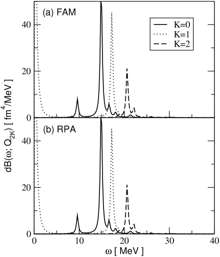
Figure 1: IS quadrupole strength distribution for ²⁰Ne. The solid, dotted, dashed lines indicate those with $K=0$, 1, and 2, respectively. Results of two kinds of calculations, (a) the finite amplitude method (FAM) and (b) the conventional RPA, are compared.

In Fig. 1(a), we show results for the IS quadrupole strength distribution. There is a NG mode in the $K=1$ sector, corresponding to the nuclear rotation. This is clearly seen in the response of the $K=1$ mode, having a large peak near $\omega=0$. The RPA correlation brings the lowest one-particle-one-hole (1p1h) excitation at $E_{x}=4.5$ MeV down to zero. The response function for the $K=1$ mode was not obtained by the small-amplitude TDHF method in Ref. Nakatsukasa and Yabana (2005), because the nucleus actually rotates in real time, that violates the small-amplitude approximation. This is an advantage of the present method over the time-dependent approach. The lowest intrinsic (physical) excitation corresponds to the $K=2$ mode at $\omega=8$ MeV which is close to energy of the 1p1h excitation. This suggests that the correlation effect is weak for this mode, supported by a small $K=2$ quadrupole strength at $\omega=8$ MeV. In contrast, the next lowest mode at $E_{x}=9.6$ MeV with $K=0$ is somewhat lowered by the correlation and exhibit a larger strength. Ref. Shinohara et al. (2006) shows results of configuration mixing calculation with the BKN interaction, indicating $J^{\pi}=0^{+}$ around $E_{x}=7$ MeV and $J^{\pi}=2^{+}$ state near 8 MeV. Large peaks at $\omega=15\sim 22$ MeV should correspond to the IS giant quadrupole resonance. It clearly shows deformation splitting; the $K=0$ peak at lowest, the $K=1$ in the middle, and the $K=2$ at the highest energy.

Now, let us demonstrate accuracy of the present finite amplitude method. In Fig. 1, results of the conventional RPA, which explicitly estimates the residual interactions $\delta h/\delta\rho$, are also presented in the panel (b). These two kinds of calculations, (a) and (b), provide identical results in the accuracy of three to four digits.

III.3.2 Isoscalar dipole and octupole response: Removal of NG modes

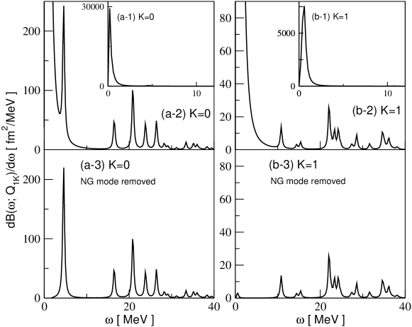
Figure 2: IS compressional dipole strength distribution for ²⁰Ne. Strengths associated with the $K=0$ modes are shown in the left (a) and those with $K=1$ in the right (b). The upper panels show strengths calculated with $\delta\rho_{\rm cal}(\omega)$, while the lower panels, (a-3) and (b-3), show those calculated with $\delta\rho_{\rm phy}(\omega)$ in Eq. (44). See text for details.

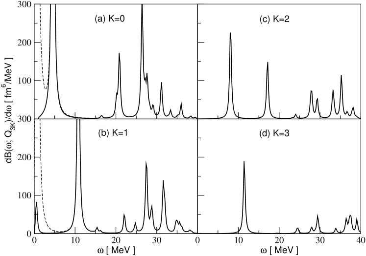
Figure 3: IS octupole strength distribution for ²⁰Ne. Strengths associated with the $K=0$, 1, 2, and 3 octupole modes are shown in the panels (a), (b), (c), and (d), respectively. In the panels (a) and (b), the strengths calculated with $\delta\rho_{\rm cal}(\omega)$ are presented by dotted lines, while those with $\delta\rho_{\rm phy}(\omega)$ are by solid lines.

Next, we show the strength distribution for the isoscalar compressional dipole mode. This mode has been of significant interest because its energy is related to the compressibility of nuclear matter, providing information independent from the monopole resonance. The compressional modes in spherical nuclei have been extensively studied with the continuum RPA calculations van Giai and Sagawa (1981); Hamamoto et al. (1998); Shlomo and Sanzhur (2002). However, these calculations are not fully self-consistent, thus, need to remove mixture of the NG (translational) components by modifying the dipole operator. This produces some ambiguity in their results. In fact, the importance of the full self-consistency has been stressed for the compressional modes Agrawal et al. (2003); Agrawal and Shlomo (2004). So far, our understanding of the compressional dipole mode is still obscure and further studies are needed. In this section, we show a fully self-consistent calculations for deformed nuclei.

In Fig. 2, the compressional dipole strength is shown, $K=0$ mode at the left (a) and $K=1$ at the right (b). There are the NG modes associated with the translational symmetry breaking near $\omega=0$, seen in Figs. 2 (a-1) and (b-1). These NG peaks are so huge that other peaks are invisible in these insets. The vertical axis is magnified in the panels (a-2) and (b-2). The giant resonance peaks are spread over $\omega=16\sim 30$ MeV for $K=0$ and $20-40$ MeV for $K=1$. There is a sharp peak at $\omega=4.5$ MeV, which is embedded in the tail of the NG mode. In order to estimate the strength carried by this state, we need to separate out the contribution from the NG mode. This is done by using the prescription described in Sec. II.4, adopting the center-of-mass coordinates and the total linear momenta (3 NG modes). Strength associated with the “physical” transition density $\delta\rho_{\rm phy}(\omega)$ is shown in Fig. 2 (a-3) and (b-3). The large strength of translational modes near $\omega=0$ is properly removed. The other physical peaks with finite $\omega$ are unchanged, which indicates that there is very little mixture of the NG modes because our calculation is fully self-consistent. Now, we may identify the $K=0$ peak at $\omega=4.5$ MeV as an isolated peak.

Finally, we show IS octupole strength distribution with $K=0$, 1, 2, and 3 in Fig. 3. The lowest octupole state is at $\omega=4.5$ MeV with $K=0$, and the second lowest is at $\omega=8.1$ MeV with $K=2$. These results are similar to that of the variation-after-parity-projection calculation Takami et al. (1996) and that of the configuration-mixing calculation Shinohara et al. (2006). Experimentally, the band head of the $K=2$ band ($J^{\pi}=2^{-}$) is observed at $E_{x}=5.0$ MeV and that of $K=0$ ($J^{\pi}=1^{-}$) is at $E_{x}=5.8$ MeV. The BKN interaction, that does not contain the spin-orbit force, is able to reproduce the $K=0$ state in a reasonable accuracy, however, fails to provide a quantitative description for the $K=2$ state. This suggests that the spin-orbit force does not play an important role for the $K=0$ state. In fact, the parity-projected HF calculation with the Skyrme interaction has confirmed very small contribution of the spin-orbit force in this $K^{\pi}=0^{-}$ state Ohta et al. (2004).

Since the nucleus is deformed, the dipole modes are coupled to the octupole modes. We may identify peaks at the same positions in Figs. 2 and 3 for the $K=0$ and $K=1$. We see a small spurious $K=1$ peak near $\omega=0$, even after removing the NG components (solid line in Fig. 3(b)). However, the peak height of the NG mode is about 5,000 fm${}^{6}/$MeV. Thus, more than 98 % of the NG strength is actually removed. We can say that the method in Sec. II.4 also works for octupole modes.

IV Conclusion and discussion

We have presented a new numerical approach to the RPA calculation, “finite amplitude method”. The finite amplitude method does not require complicated programming for complex residual interactions. Instead, it resorts to the numerical derivation of the residual interaction (induced field), $\delta h/\delta\rho\cdot\delta\rho$. The most advantageous feature of the present method is its feasibility of programming a computer code. The RPA calculation can be accomplished with a minor extension of the static HF computer code, to construct the HF Hamiltonian with independent bra and ket single-particle states.

Here, we would like to make a remark on the meaning of different bra and ket states. This does not mean matrix elements between different Slater determinants which are rather complicated. These “off-diagonal” elements are necessary for configuration-mixing calculations, such as the generator-coordinate method. The finite amplitude method does not require these. All we need is “diagonal” matrix elements of a certain one-body operator, $\hat{o}$, in the linear order with respect to variation of the single-particle states,

$$\sum_{i=1}^{A}\langle{\psi_{i}}|\hat{o}|{\psi_{i}}\rangle\approx\sum_{i=1}^{A}\langle{\phi_{i}}|\hat{o}|{\phi_{i}}\rangle+\sum_{i=1}^{A}\langle{\delta\psi_{i}}|\hat{o}|{\phi_{i}}\rangle+\sum_{i=1}^{A}\langle{\phi_{i}}|\hat{o}|{\delta\psi_{i}}\rangle.$$ (61)

In order to calculate the second and the third terms in the r.h.s. separately, we need to input independent bra and ket single-particle states. This can be achieved by a minor extension of the static HF code.

The method has been applied to calculations of the isoscalar dipole, quadrupole, and octupole response functions. Since the adopted interaction is rather schematic, we do not discuss here calculated properties of these modes. Instead, we would like to emphasize characteristic features of the finite amplitude method. First of all, the transition density coupled to the NG modes can be calculated without any special treatment. As is seen in the quadrupole ($K=1$) and octupole modes ($K=0$ and 1) in Figs. 1 and 3, the NG modes appear in responses to a variety of external fields, especially for deformed nuclei. This causes a serious problem in the time-dependent calculation of the small-amplitude TDHF Nakatsukasa and Yabana (2005). If we want to remove the strength associated with the NG modes, we can use the prescription presented in Sec. II.4. This has been demonstrated in the dipole and octupole strength distributions. Second, since we do not calculate the residual interaction explicitly, it is easy to carry out the fully self-consistent RPA calculation for realistic interactions including spin-orbit, derivative, and Coulomb terms. The implementation of the present method does not depend on the complexity of the interactions. For instance, the compressional dipole mode has been a long-standing problem in microscopic calculations van Giai et al. (2001). The problem is related to difficulties in the fully self-consistent treatment and the coupling to the translational modes. Our new approach may provide a tool to clarify this point. Last but not least, the finite amplitude method is an efficient method to calculate the strength distribution. We may control the necessary energy resolution by the smoothing parameter $\Gamma$. The numerical application to the BKN functional shows that its efficiency is next to the time-dependent method, better than the other methods including the Green’s function method Nakatsukasa and Yabana (2005) and the diagonalization method Muta et al. (2002). The diagonalization of the RPA matrix is very efficient if we are interested in only a few lowest states, however, it becomes more and more difficult for higher excitation energies.

For future developments, it is interesting to combine the present method with the absorbing-boundary-condition approach in Ref. Nakatsukasa and Yabana (2005). This enables us to calculate response in the continuum, overcoming difficulties in the time-dependent method. It is also very interesting to extend the method in the HF scheme to the one in the Hartree-Fock-Bogoliubov framework. In this paper, we adopt a simple interaction to check the method, but the finite amplitude method shows its real power for a complex density functional. Applications of the method to the realistic Skyrme functionals are under progress at present and will be published in near future.