Electro-disintegration following beta-decay

Abstract

I show that the disintegration of weakly-bound nuclei and the ionization of weakly-bound atomic electrons due to their interaction with leptons from beta decay is a negligible effect.

The disintegration of weakly bound nuclei with small neutron separation energy in stars can impose limits to the stellar scenario where these nuclei exist. Beta-decay already sets stringent limits on the existence of nuclei very far from the line of stability (see, e.g. Ri02 ). Here I discuss an additional effect, namely the restrictions imposed by final state interactions of the beta-particle with the daughter nucleus. Electrons observed in beta-decay can have enough kinetic energy to induce the dissociation of the daughter nucleus with small separation energy. If this process is proven to be relevant, it would lead to the existence of voids in the elemental abundance close to the drip-line.

The basic assumptions adopted here are that the excitation (dissociation) of a nucleus following beta-decay is sequential and that it can be described as a two-step process, so that the transition rate is given by

$$W_{i\rightarrow m\rightarrow f}=W_{i\rightarrow m}^{\left(\beta\right)}\cdot P_{m\rightarrow f}^{(e)}$$

where $W_{i\rightarrow m}^{\left(\beta\right)}$ is the usual beta-decay transition rate from an initial nuclear state $i$ to an intermediary state $m$, and $P_{m\rightarrow f}^{(e)}$ is the probability for the nuclear excitation from $m$ to a final state $f$ by the interaction of the nucleus with the outgoing electron (positron).

The beta-particle is described by a spherically symmetric outgoing wave, that favors monopole transitions in the daughter nucleus. We neglect retardation and assume that the electron (positron) energy is much larger than the excitation energy. The outgoing electron wave will generate a time-dependent monopole wake field whose interaction with the nucleus has the usual form $V_{e}=e_{eff}/r$, where $e_{eff}$ is the effective charge for the transition. The effective charge arises due to the modification of the charge radius of the nucleus after nucleon emission. An accurate value of the effective charge depends strongly on the nuclear properties Ta72 . For simplicity, I will assume $e_{eff}\sim e$.

Because of the assumed spherical symmetry, the Coulomb field of the electron (positron) only exists outside the outgoing electron wavefront. Therefore, in first-order time-dependent perturbation theory, the excitation amplitude $A_{m\rightarrow f}^{(e)}$ is given by

$$A_{m\rightarrow f}^{(e)} =\frac{1}{i\hbar}e^{2}\int dt\exp\left[i\left(E_{f}-E_{m}\right)t/\hbar)\right]$$

$$\int_{r>r_{e}(t)}d^{3}r\ \frac{1}{r}\Psi_{f}^{\ast}\left(\mathbf{r}\right)\Psi_{m}\left(\mathbf{r}\right),$$ (1)

where we set up the spin angular part of the matrix element equal to 1. $\Psi_{j}\left(\mathbf{r}\right)$ denotes the nuclear wavefunction, $E_{j}$ the nuclear energy of state $j$, $r_{e}$ is the electron and $r$ the internal nuclear coordinate.

We use a simplified nuclear model for the nuclear wavefunction $\Psi\left(\mathbf{r}\right)$ which captures the essence of the process. The wavefunction for the state $m$ is taken as an $s$-wave Hulthén   wave function HS57

$$\Psi_{m}\left(\mathbf{r}\right)=N\frac{u_{m}(r)}{r}=N\frac{\left(e^{-\alpha r}-e^{-\beta r}\right)}{r}.$$ (2)

The term $e^{-\beta r}$ modifies the asymptotic form $e^{-\alpha r}$ at small distances in such a way that $u_{m}(0)=0$, and more specifically $u_{m}\sim r$, as is reasonable for $s$ waves. Moreover, the parameter $\alpha$ is given in terms of the separation energy of the nucleon from the nucleus by the equation $S_{n}=\hbar^{2}\alpha^{2}/2m_{n}$, where $m_{n}$ is the reduced nucleon-nucleus mass and $\beta$ can be determined from the effective range parameter, $r_{0}$, as approximately HS57 ; Adl70

$$\beta=\frac{3-\alpha r_{0}+\left(\alpha^{2}r_{0}^{2}-10\alpha r_{0}+9\right)^{1/2}}{2r_{0}},$$ (3)

and in general $\beta\gg 1$. Similarly, the normalization constant can be expressed in terms of the effective range as $N^{2}=\alpha\left[2\pi(1-\alpha r_{0})\right]^{-1}$. In the following numerical calculations we will use $r_{0}=3$ fm, a typical value for nuclear systems.

The final wavefunction is an outgoing spherical wave,

$$\Psi_{f}\left(\mathbf{r}\right)=\frac{1}{2ikr}\exp\left(ikr\right)$$ (4)

where $k$ is related to the relative kinetic energy of the final state by $\varepsilon=\hbar^{2}k^{2}/2m_{n}$.

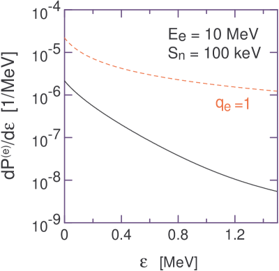
Figure 1: (Color online) Energy spectrum of continuum states produced by electro-dissociation following a beta-decay with electron (positron) energy $E_{e}=10$ MeV. The initial state is bound by 100 keV. The dashed curve is obtained with the approximation of eq. 7.

If $v_{e}$ denotes the electron velocity, assumed to remain undisturbed by the energy transfer to the excitation, the time dependence of the electron position is $r_{e}=v_{e}t$. The first integral in eq. 1 can be expressed in terms of the exponential integral function, $\operatorname{Ei}\left(x\right)$, as

$$A_{m\rightarrow f}^{(e)}\left(E_{e},S_{n},\epsilon\right) =\frac{2\pi e^{2}N}{\hbar kv_{e}}\int_{0}^{\infty}dr\ q_{e}\left(\lambdabar_{e},r\right)\ \exp\left(i\frac{\omega r}{v_{e}}\right)$$

$$\left[\operatorname{Ei}\left(-ar\right)-\operatorname{Ei}\left(-br\right)\right],$$ (5)

where $E_{e}$ is the electron (positron) energy, $a=\alpha+ik$ and $b=\beta+ik$ and we use the short notation $\omega=\left(E_{f}-E_{m}\right)/\hbar,$ such that $\hbar\omega=S_{n}+\varepsilon$. Note that we have introduced an electron-charge distribution $\ q\left(\lambdabar_{e},r\right)$ which has the following meaning. When the electron (positron) is produced in beta-decay its charge is homogeneously distributed within a sphere of the size of its Compton wavelength $\lambdabar_{e}=\hbar/\gamma m_{e}c$, where $\gamma=\left(1-v_{e}^{2}/c^{2}\right)^{-1/2}.$ This is based on the uncertainty principle, which introduces a smearing out of the electron coordinate within a region equal to its wavelength. This condition implies that

$$q_{e}\left(\lambdabar_{e},r\right)=\left\{\begin{array}[c]{c}r^{3}/\lambdabar_{e}^{3},\text{ \ \ \ \ for \ \ }r<\lambdabar_{e}\\ 1\text{, \ \ \ \ for \ \ }r\geqslant\lambdabar_{e}\end{array}\right..$$ (6)

If $q_{e}=1$ is used, the integral in eq. 5 can be performed analytically. One gets

$$\frac{v_{e}}{2\omega}\left\{2\arctan\left(\frac{\omega}{v_{e}a}\right)-2\arctan\left(\frac{\omega}{v_{e}b}\right)\right.$$

$$\left.-i\left[\ln\left(1+\frac{\omega^{2}}{v_{e}^{2}a^{2}}\right)-\ln\left(1+\frac{\omega^{2}}{v_{e}^{2}b^{2}}\right)\right]\right\}.$$ (7)

Finally, the dissociation probability is given by

$$P_{m\rightarrow f}^{(e)}\left(E_{e},S_{n}\right) =\int d\varepsilon\rho\left(\varepsilon\right)\left|A_{m\rightarrow f}^{(e)}\right|^{2}$$

$$=\frac{\left(2m_{n}\right)^{3/2}}{(2\pi\hbar)^{3}}\int_{0}^{\infty}\left|A\left(E_{e},S,\varepsilon\right)\right|^{2}\sqrt{\varepsilon}d\varepsilon,$$ (8)

where $\rho\left(\varepsilon\right)=\left(2m_{n}\right)^{3/2}\sqrt{\varepsilon}d\varepsilon/(2\pi\hbar)^{3}$ is the density of final states of the nucleon-nucleus system.

Figure 1 shows the energy spectrum, $dP^{(e)}/d\varepsilon$, of continuum states produced by electro-dissociation following a beta-decay with electron (positron) energy $E_{e}=10$ MeV. The initial state is bound by 100 keV. The dashed curve is obtained with the approximation of eq. 7. One sees that, as expected, neglecting the wave character of the electron (i.e., using eq. 7) leads to a large overestimation of the excitation probabilities. Using the value of $q_{e}$ as given by eq. 6 leads to a steeper decrease of states with larger energy. Obviously, for too large excitation energies of the nucleus the total energy is not conserved and the formalism described above is not appropriate.

$S_{n}\$[keV]	$P^{(e)}$
10	$9.3\times 10^{-7}$
70	$4.8\times 10^{-7}$
160	$1.9\times 10^{-7}$
310	$7.3\times 10^{-8}$

Table 1: Dissociation probability of a loosely-bound nucleus as a function of the neutron separation energy $S_{n}$ in keV for an electron with energy $E_{e}=10$ MeV.

Table 1 shows the dissociation probability of a loosely-bound nucleus as a function of the neutron separation energy $S_{n}$ in keV for an electron (positron) with energy $E_{e}=10$ MeV. The probabilities are very small, even for 10 keV separation energy. This rules out nuclear dissociation following beta-decay as a relevant effect in beta-decay processes close to the drip line. A full quantum mechanical calculation will not change this conclusion as the main ingredients of the effect have been taken into account above. Also, for charged particle (e.g., emission of a proton) this effect is further suppressed due to the Coulomb barrier.

Naïvely, this calculation can be used to estimate the probability that the beta-particle ionizes the atom by ejecting one of its outer electrons. One can use the equations above and just replace the nucleon mass by the electron mass (using $r_{0}=0$). While the Hulthén wavefunction, eq. 2, is a good approximation for a loosely bound electron, the scattering wave, eq. 4, is obviously wrong as it does not account for the (screened) charge of the residual atom. An estimate of the Coulomb effect follows by adding a Coulomb phase, $(e^{2}/\hbar v_{e})\ln\left(2k_{e}r\right)$, to the exponent in eq. 4. It has been checked numerically that this changes the results by only few percent. Moreover, an exact treatment of Coulomb distortion tends to decrease the magnitude of the ionization probabilities in projectile impact processes BS77 .

Results for atomic ionization following beta decay are shown in Table 2 as a function of the beta-particle energy assuming a loosely bound electron with separation energy of $S_{e}=1$ eV. One sees, as expected, that the ionization probability decreases with the beta-decay electron energy. The obvious reason is the increase of the wavelength mismatch between the emitted electron and that of the beta-particle as the energy of the later increases. The ionization probability remains small even when the beta-particle has small energy.

$E_{e}$	$P^{(e)}$
10 eV	$4.7\times 10^{-8}$
50 keV	$6.3\times 10^{-10}$
1 MeV	$1.09\times 10^{-10}$
5 MeV	$1.97\times 10^{-11}$

Table 2: Ionization probability of a loosely-bound atom ($S_{e}=1$ eV) as a function of the beta-particle energy $E_{e}$.

We conclude that the excitation, or dissociation, of nuclei as well as the atomic ionization by the electron (or positron) emitted in beta-decay processes are negligible effects. A calculation using Feynman diagram techniques with proper account of relativistic effects and energy conservation is very unlikely to change these conclusions. The same line of thought applies to the consideration of higher multipole interactions.

Acknowledgements

I thank Alex Brown for bringing this problem to my attention and to Akram Mukhamezhanov for useful discussions. This research was supported by the U.S. Department of Energy under contract No. DE-AC05-00OR22725 (Oak Ridge National Laboratory) with UT-Battelle, LLC., and by DE-FC02-07ER41457 with the University of Washington (UNEDF, SciDAC-2).

References

- (1) K. Riisager, Eur. Phys. J. A 15, 75 (2002).
- (2) L. Hulthén and M. Sugawara, in Handbuch der Physik, edited by S. Flugge (Springer-Verlag, Berlin, 1957), vol. 39, p. 14.
- (3) R.J. Adler, B.T. Chertok, and H.C. Miller, Phys. Rev. C 2, 69 (1970).
- (4) J. W. Tape, E. G. Adelberger, D. Burch and L. Zamick, Phys. Rev. Lett. 29, 878 (1972).
- (5) H. Bethe and E.E. Salpeter, Quantum Mechanics of One- and Two-electron Atoms (Plenum, New York, 1977).