Virtues and Flaws of the Pauli Potential

Abstract

Quantum simulations of complex fermionic systems suffer from a variety of challenging problems. In an effort to circumvent these challenges, simpler “semi-classical” approaches have been used to mimic fermionic correlations through a fictitious “Pauli potential”. In this contribution we examine two issues. First, we address some of the inherent difficulties in a widely used version of the Pauli potential. Second, we refine such a potential in a manner consistent with the most basic properties of a cold Fermi gas, such as its momentum distribution and its two-body correlation function.

I Introduction

Insights into the complex and fascinating dynamics of Coulomb frustrated systems across a variety of disciplines are just starting to emerge (see, for example, Ref. Jamei et al. (2005) and references therein). In the particular case of neutron stars, one is interested in describing the equation of state of neutron-rich matter across an enormous density range using a single underlying theoretical model. In recent simulations we have resorted to a classical model that, while exceedingly simple, captures the essential physics of Coulomb frustration and nuclear saturation Horowitz et al. (2004a, b); Horowitz et al. (2005). The model includes competing interactions consisting of a short-range nuclear attraction (adjusted to reproduce nuclear saturation) plus a long-range Coulomb repulsion. The charge-neutral system consists of electrons, protons, and neutrons, with the electrons (which at these densities are no longer bound) modeled as a degenerate free Fermi gas.

So far, the only quantum effect that has been incorporated into this “semi-classical” model is the use of an effective temperature to simulate quantum zero-point motion. The main justification behind the classical character of the simulations is the heavy nature of the nuclear clusters. Indeed, at the low densities of the neutron-star crust, the de Broglie wavelength of the heavy clusters is significantly smaller than their average separation. However, this behavior ceases to be true in the transition region from the inner crust to the outer core. At the higher densities of the outer core, the heavy clusters are expected to “melt” into a collection of isolated nucleons with a de Broglie wavelength that becomes comparable to their average separation. Thus, fermionic correlations are expected to become important in the crust-to-core transition region. Unfortunately, in contrast to classical simulations that routinely include thousands — and even millions — of particles, full quantum-mechanical simulations of many-fermion systems suffer from innumerable challenges (see Ref. Grotendorst et al. (2002) and references therein). In an effort to “circumvent” — although not solve — some of these formidable challenges, classical simulations of heavy-ion collisions and of the neutron-star crust have resorted to a fictitious “Pauli potential”. Within the realm of nuclear collisions, the first such simulations were those of Wilets and collaborators Wilets et al. (1977). Other simulations with a more refined Pauli potential have followed Dorso et al. (1987); Boal and Glosli (1988); Peilert et al. (1992); Maruyama et al. (1998); Watanabe et al. (2003), but the spirit has remain the same: introduce a momentum dependent, two-body Pauli potential that penalizes the system whenever two identical nucleons get too close to each other in phase space.

A goal of the present contribution is to show that the demands imposed by such a Pauli potential are too weak to reproduce some of the most basic properties of a zero-temperature (or cold) Fermi gas. Thus, we aim at refining such a potential in a manner that three fundamental properties of a cold Fermi gas be reproduced. These are: ($i$) the kinetic energy (as others have done before us), ($ii$) the momentum distribution, and ($iii$) the two-nucleon correlation function.

The manuscript has been organized as follows. In Sec. II, some of the basic properties of a free Fermi gas are discussed. As our classical simulations must by necessity be carried out at finite temperature, a Sommerfeld expansion is used to compute low-temperature corrections to these observables. The section concludes with a review of the “standard” form of the Pauli potential, its flaws, and the measures that we take to overcome these flaws. In Sec. III, results for the kinetic energy, momentum distribution, and two-body correlation function are presented and contrasted against exact analytic results. Conclusions and possible future directions are presented in Sec. IV.

II Formalism

The present section starts with a brief overview of some fundamental properties of a low-temperature Fermi gas Pathria (1996). Next, a fictitious Pauli potential is introduced and constrained to reproduce these properties via a purely classical simulation. In particular, special emphasis is placed on the necessary modifications to the “standard” Pauli potential that are required to reproduce such fundamental properties.

II.1 Free Fermi Gas

The zero temperature Fermi gas is the simplest many-fermion system. Such a system displays no correlations beyond those imposed by the Pauli exclusion principle and is described by the following free Hamiltonian:

$$H=\sum_{i=1}^{N}\frac{{\bf p}_{i}^{2}}{2m}\;.$$ (1)

Here $m$ is the mass of the fermion and $N$ denotes the (large) number of particles in the system. As no interaction of any sort exists among the particles, the eigenstates of the system are given by a product of (single-particle) momentum eigenstates, suitably antisymmetrized to fulfill the constraints imposed by the Pauli principle. For simplicity, we assume that the fermions reside in a very large box of volume $V\!=\!L^{3}$ and that the momentum eigenstates satisfy periodic boundary conditions. We will be interested in the thermodynamic limit of $N\!\rightarrow\infty$ and $V\!\rightarrow\infty$, but with their ratio fixed at a specific value of the number density $\rho\!\equiv\!N/V$.

The (“box”) normalized momentum eigenstates are simple plane waves. That is,

$$\varphi_{\bf p}({\bf r})=\frac{1}{\sqrt{V}}\,e^{i{\bf p}\cdot{\bf r}}\;.$$ (2)

Given that the eigenvalue problem is solved in a finite box using periodic boundary conditions, the resulting single-particle momenta are quantized as follows:

$${\bf p}({\bf n})=\frac{2\pi}{L}{\bf n}=\frac{2\pi}{L}(n_{x},n_{y},n_{z})\;,\;\;{\rm with}\;n_{i}=0,\pm 1,\pm 2,\ldots$$ (3)

with the corresponding single-particle energies given by $\epsilon({\bf p})={\bf p}^{2}/2m$.

Up to this point the spin/statistics of the particles has not come into play. We are now interested in describing the ground state of a system of $N$ non-interacting, identical fermions and the resulting many-body correlations. Such a zero-temperature state is obtained by placing all particles in the lowest available momentum state, consistent with the Pauli exclusion principle. Using fermionic creation and annihilation operators satisfying the following anti-commutation relations Fetter and Walecka (1971),

$$\Big{\{}A_{\bf p},A_{{\bf p}^{\prime}}^{\dagger}\Big{\}}=\delta_{{\bf p},{\bf p}^{\prime}}\;\;{\rm and}\;\Big{\{}A_{\bf p},A_{{\bf p}^{\prime}}\Big{\}}=\Big{\{}A_{\bf p}^{\dagger},A_{{\bf p}^{\prime}}^{\dagger}\Big{\}}=0\;,$$ (4)

the ground state of the system may be written as follows:

$$|\Phi_{\rm FG}\rangle=\prod_{{\bf p}=0}^{{\bf p}_{\rm F}}A_{\bf p}^{\dagger}|\Phi_{\rm vac}\rangle\;,$$ (5)

where $|\Phi_{\rm vac}\rangle$ represents the (non-interacting) vacuum state and the Fermi momentum ${\bf p}_{\rm F}$ denotes the momentum of the last occupied single-particle state. Note that henceforth, no intrinsic quantum number (such as spin and/or isospin) will be considered. In essence, one assumes that all intrinsic degrees of freedom have been “frozen”, thereby concentrating on a single fermionic species (such as neutrons with spin up). In what follows, we compute expectation values of various quantities in the Fermi gas ground state ($|\Phi_{\rm vac}\rangle$).

We start by computing the Fermi momentum ${\bf p}_{\rm F}$ in terms of the number density of the system $\rho\!=\!N/V$. That is,

$$N=\sum_{{\bf n}}n_{\rm FD}({\bf n})\mathop{\longrightarrow}_{V\rightarrow\infty}V\int\frac{d^{3}p}{(2\pi)^{3}}n_{\rm FD}({\bf p})\mathop{=}_{T=0}V\frac{p_{\rm F}^{3}}{6\pi^{2}}\;,$$ (6)

or equivalently,

$$p_{\rm F}=\left(6\pi^{2}\rho\right)^{1/3}\;.$$ (7)

Note that in Eq. (6) $n_{\rm FD}({\bf p})$ denotes the Fermi-Dirac occupancy of the single-particle state denoted by ${\bf p}$ (or ${\bf n}$) and the thermodynamic limit has been assumed. As all ground-state observables will be computed over a spherically-symmetric Fermi sphere, we define the Fermi-Dirac momentum distribution $f(q)$ as follows:

$$f(q)=3q^{2}n_{\rm FD}(q)\;,\;\;{\rm with}\;\int_{0}^{\infty}f(q)dq=1\;,$$ (8)

where the dimensionless quantity $q\!\equiv\!p/p_{\rm F}$ is the momentum of the particle in units of the Fermi momentum.

All classical simulations performed and reported in the next sections must be carried out by necessity at finite temperature. Thus, we now incorporate finite temperature corrections to the various observables of interest. For temperatures $T$ that are small relative to the Fermi temperature $T_{\rm F}$ (with $T_{\rm F}\!\equiv\!\epsilon_{\rm F}$), finite-temperature corrections may be implemented by means of a Sommerfeld expansion Pathria (1996). For example, to lowest order in $\tau\!\equiv\!T/T_{\rm F}$ the momentum distribution becomes

$$f(q,\tau)=\frac{3q^{2}}{\exp{\displaystyle\left[{\left(q^{2}-1+\frac{\pi^{2}}{12}\tau^{2}\right)\Big{/}\tau}\right]+1}}\,\mathop{\longrightarrow}_{\tau\rightarrow 0}\ 3q^{2}\Theta(1-q)\;.$$ (9)

Here $\Theta(x)$ is the “Heaviside step function” appropriate for a zero-temperature Fermi gas. Similarly, the energy-per-particle of a “cold” Fermi gas may be readily computed. One obtains Pathria (1996)

$$E/N=\epsilon_{\rm F}\int_{0}^{\infty}q^{2}f(q)dq=\frac{3}{5}\epsilon_{\rm F}\left[1+\frac{5\pi^{2}}{12}\tau^{2}+{\cal O}(\tau^{4})\right]\;,$$ (10)

where the Fermi energy is defined by $\epsilon_{\rm F}\!=\!p_{\rm F}^{2}/2m$.

The last Fermi-gas observable that we focus on is the “two-body correlation function” $g(r)$. This observable measures the probability of finding two particles at a fixed distance $r$ from each other. Moreover, the two-body correlation function is a fundamental quantity whose Fourier transform yields the static structure factor, an observable that may be directly extracted from experiment. As such, the two-body correlation function is the natural meeting place of theory, experiment, and computer simulations Vesely (2001). The two-body correlation function may be derived from the density-density correlation function Fetter and Walecka (1971). That is,

$$g(r)=\frac{1}{\rho^{2}}\rho_{2}({\bf x},{\bf y})=\frac{1}{\rho^{2}}\Big{\langle}\hat{\psi}^{\dagger}({\bf x})\hat{\psi}^{\dagger}({\bf y})\hat{\psi}({\bf y})\hat{\psi}({\bf x})\Big{\rangle}\;,$$ (11)

where $\hat{\psi}({\bf x})$ is a fermionic field operator and the Dirac brackets denote a thermal expectation value. As the two-body correlation function for a non-interacting Fermi gas may be readily evaluated at zero temperature Fetter and Walecka (1971), we only provide its extension to finite temperatures. To lowest order in $\tau\!\equiv\!T/T_{\rm F}$ (and for a single fermionic species) one obtains

$$g(r)=1-\left(3\,\frac{j_{1}(z)}{z}\right)^{2}\left[1-\frac{\pi^{2}}{12}z^{2}\tau^{2}\right]\;,$$ (12)

where $z\!\equiv\!p_{\rm F}r$ and $j_{1}(z)$ is the spherical Bessel function of order $n\!=\!1$, namely,

$$j_{1}(z)=\frac{\sin(z)}{z^{2}}-\frac{\cos(z)}{z}\;.$$ (13)

Equations (9), (10), and (12) display the three fundamental observables of a cold Fermi gas that we aim to reproduce in this work via a momentum-dependent, two-body Pauli potential. Note that in most (if not all) earlier studies of this kind, only the kinetic energy of the Fermi gas [Eq. (10)] was used to constrain the parameters of the Pauli potential Wilets et al. (1977); Dorso et al. (1987); Boal and Glosli (1988); Peilert et al. (1992); Maruyama et al. (1998); Watanabe et al. (2003). We are unaware of any earlier effort at including more sensitive Fermi-gas observables to constrain the parameters of the model. Clearly, it should be possible to reproduce the second moment of the distribution (i.e., the kinetic energy) even with an incorrect momentum distribution. Thus, while we build on earlier approaches, we also highlight some of their shortcomings.

II.2 Pauli Potential: A New Functional Form

In the previous section the wave function of a zero-temperature Fermi gas was introduced as follows:

$$|\Phi_{\rm FG}\rangle=\prod_{{\bf p}=0}^{{\bf p}_{\rm F}}A_{\bf p}^{\dagger}|\Phi_{\rm vac}\rangle\;.$$ (14)

Essential to the dynamical behavior of the system are the anti-commutation relations [Eq. (4)] that enforce the Pauli exclusion principle (i.e., $(A_{\bf p}^{\dagger})^{2}\!\equiv\!0$). As it is often done, one may project the above “second-quantized” form of the many-fermion wave-function into configuration space to obtain the well-known Slater determinant. That is,

$$\Phi_{FG}({\bf p}_{1},\dots,{\bf p}_{N};{\bf r}_{1},\dots,{\bf r}_{N})=\frac{1}{\sqrt{N!}}\left|\begin{matrix}\varphi_{{\bf p}_{1}}({\bf r}_{1})&\ldots&\varphi_{{\bf p}_{1}}({\bf r}_{N})\\ \vspace{-0.1cm}.&\ldots&.\\ \vspace{-0.1cm}.&\ldots&.\\ \vspace{-0.1cm}.&\ldots&.\\ \vspace{+0.1cm}\varphi_{{\bf p}_{N}}({\bf r}_{1})&\ldots&\varphi_{{\bf p}_{N}}({\bf r}_{N})\end{matrix}\right|\;,$$ (15)

where the single-particle wave-functions $\varphi_{\bf p}({\bf r})$ are the (“box”) normalized plane waves defined in Eq. (2). The Slater determinant embodies important correlations that were discussed in the previous section and that we aim to incorporate into our classical simulations. These are:

(a) At zero temperature, only momentum states having a magnitude $|{\bf p}|$ less than the Fermi momentum $p_{\rm F}$ are occupied; the rest are empty.

(b) As a consequence of the Pauli exclusion principle [$(A_{\bf p}^{\dagger})^{2}\!\equiv\!0$], the probability that two fermions share the same identical momentum is equal to zero. Mathematically, this result follows from the fact that the wave-function vanishes whenever two rows of the Slater determinant are equal to each other.

(c) Similarly, the wave-function also vanishes whenever two columns of the Slater determinant are identical. This fact precludes two fermions from occupying the same exact location in space.

The first two properties are embedded in the momentum distribution of Eq. (9), namely, a quadratic momentum distribution sharply peaked at the Fermi momentum $p_{\rm F}$ (recall that such a momentum distribution emerges after folding the Heaviside step function with the phase space factor). The third property induces spatial correlations that are captured by the two-body correlation function $g(r)$ of Eq. (12). Indeed, the two-body correlation function is related to the integral of the Slater determinant over all but two of the coordinates of the particles (e.g., ${\bf r}_{1}$ and ${\bf r}_{2}$). Clearly, the Slater determinant vanishes whenever ${\bf r}_{1}={\bf r}_{2}$, and so does the two-body correlation function at $r\!=\!|{\bf r}_{1}-{\bf r}_{2}|\!\equiv\!0$. It is the aim of this contribution to build a Pauli potential that incorporates these three fundamental properties of a free Fermi gas.

However, before doing so, we briefly review the Pauli potential introduced by Wilets and collaborators — and used by others with minor modifications — to simulate the collisions of heavy ions and the properties of neutron rich matter at sub-saturation densities. Such a Pauli potential is given by a sum of momentum-dependent, two-body terms of the following form:

$$V_{\rm Pauli}({\bf p}_{1},\dots,{\bf p}_{N};{\bf r}_{1},\dots,{\bf r}_{N})=\sum_{i<j=1}^{N}V_{0}\exp(-s_{ij}^{2}/2)\;,$$ (16)

where $V_{0}\!>\!0$ and the dimensionless phase-space “distance” between points $({\bf p}_{i},{\bf r}_{i})$ and $({\bf p}_{j},{\bf r}_{j})$ is given by

$$s_{ij}^{2}\equiv\frac{|{\bf p}_{i}-{\bf p}_{j}|^{2}}{p_{0}^{2}}+\frac{|{\bf r}_{i}-{\bf r}_{j}|^{2}}{r_{0}^{2}}\;.$$ (17)

Here $p_{0}$ and $r_{0}$ are momentum and length scales related to the excluded phase-space volume that is used to mimic fermionic correlations. That is, whenever the phase-space distance between two particles is such that $s_{ij}^{2}\!\lesssim\!1$, then a penalty is levied on the system in an effort to mimic the Pauli exclusion principle. Although the parameters of this Pauli potential ($V_{0}$, $p_{0}$, and $r_{0}$) can — and have — been adjusted to reproduce the kinetic energy of a free Fermi gas, it fails (as we show later) in reproducing more sensitive Fermi-gas observables, particularly, the momentum distribution $f(p)$ and the two-body correlation function $g(r)$.

Upon closer examination, the above flaws should not come as a surprise. In our previous discussion of the Slater determinant it has been established that the probability of finding two identical fermions in the same location in space “or” with the same momenta must be identically equal to zero. Yet the Pauli potential of Eq. (16) fails to incorporate this important dynamical behavior. Indeed, the above Pauli potential imposes a penalty on the system only when both the location “and” momenta of the two particles are close to each other (i.e., $s_{ij}^{2}\!\lesssim\!1$). In particular, no penalty is imposed whenever two fermions occupy the same location in space, provided that their momenta are significantly different from each other, i.e., $|{\bf p}_{i}-{\bf p}_{j}|^{2}\!\gg\!p_{0}^{2}$. Thus, the Pauli potential of Eq. (16) will generate an incorrect two-body correlation function, namely, one with $g(r)\!\neq\!0$ as r tends to zero. By the same token, an incorrect momentum distribution will be generated, although not necessarily its second moment.

To remedy these deficiencies, a Pauli potential is now constructed so that the three properties [(a), (b), and (c)] defined above are explicitly satisfied. To this end, we introduce the following form for the Pauli potential:

$$V_{\rm Pauli}({\bf p}_{1},\dots,{\bf p}_{N};{\bf r}_{1},\dots,{\bf r}_{N}) = \sum_{i<j=1}^{N}\Big{[}V_{A}\exp(-r_{ij}/r_{0})+V_{B}\exp(-p_{ij}/p_{0})\Big{]}$$ (18)

$$+ \sum_{i=1}^{N}V_{C}\,\Theta_{\eta}(q_{i})\;,$$

where $r_{ij}\!=\!|{\bf r}_{i}-{\bf r}_{j}|$, $p_{ij}\!=\!|{\bf p}_{i}-{\bf p}_{j}|$, $q_{i}\!=\!|{\bf p}_{i}|/p_{\rm F}$, and $\Theta_{\eta}$ is a suitably smeared Heaviside-step function of the following form:

$$\Theta_{\eta}(q)\equiv\frac{1}{1+\exp[-\eta(q^{2}-1)]}\mathop{\longrightarrow}_{\eta\rightarrow\infty}\Theta(q)\;.$$ (19)

The parameters of the model $V_{A},V_{B},V_{C}$ and $r_{0},p_{0},\eta$ will be adjusted to reproduce both the momentum distribution and two-body correlation function of a low-temperature Fermi gas. Note that the phase-space dependence of the Pauli potential has been separated into a “sum” of two-body pieces, with the first acting exclusively in configuration space and the second one only in momentum space. The first term in the potential imposes a penalty as the particles get too close (of the order of $r_{0}$) to each other. Similarly, the second term in the potential penalizes particles whenever their relative momenta becomes of the order of $p_{0}$. Finally, the third “one-body” term enforces the low-temperature behavior of the Fermi gas, namely, that the probability of finding any particle with a momentum significantly larger than the Fermi momentum is vanishingly small. Most of the parameters will depend explicitly on the density of the system (see Sec. III). This reflects the complex many-body nature of the Pauli correlations and our inability to simulate them by means of a “simple” (albeit momentum dependent) two-body potential.

III Results

We start this section by listing in Table 1 the parameters of the Pauli potential. For the strength parameters, the following simple density dependence is assumed:

$$V_{i}(\rho)=V_{i}^{0}\Big{(}\rho/\rho_{0}\Big{)}^{\alpha_{i}}\;,\quad i=\{A,B,C\}\;,$$ (20)

where $\rho_{0}\!=\!\rho_{sat}/4\!=\!0.037~{}{\rm fm}^{-3}$ is the density of a single fermionic species (for example, neutrons with spin up) at nuclear-matter saturation density ($\rho_{sat}$ = 0.148 fm^-3). For the range parameters ($r_{0}$ and $p_{0}$) the following scaling relation is adopted:

$$r_{0}=\beta_{A}/p_{\rm F}\;,$$ (21a)

$$p_{0}=\beta_{B}p_{\rm F}\;.$$ (21b)

$V_{A}^{0}$	$V_{B}^{0}$	$V_{C}^{0}$	$\alpha_{A}$	$\alpha_{B}$	$\alpha_{C}$	$\beta_{A}$	$\beta_{B}$	$\eta$
13.517	1.260	3.560	0.629	0.665	0.831	0.845	0.193	30

Table 1: Strength (in MeV) and range parameters (dimensionless) for the various components of the Pauli potential. See Eqs. (18), (20), and (21). These values have been used to simulate a system of $N\!=\!1000$ identical fermions at a temperature of $\tau\!=\!T/T_{\rm F}\!=\!0.05$.

Monte-Carlo simulations for a system of $N\!=\!1000$ identical fermions at the finite (but small) temperature of $\tau\!=\!T/T_{\rm F}\!=\!0.05$ have been performed. Initially, the particles are distributed randomly throughout the box with momenta that are uniformly distributed up to a maximum momentum of the order of the Fermi momentum. After an initial thermalization phase of typically 2000 sweeps (or 2 million Monte Carlo moves for both coordinates and momenta) data is accumulated for an additional 2000 sweeps, with the data divided into 10 groups to avoid correlations among the data. It is from these 10 groups that averages and errors are generated.

III.1 Kinetic Energy

The kinetic energy of a finite-temperature Fermi gas as a function of density is displayed in Fig.1. The (black) solid line represents the analytic behavior of a free Fermi gas correct to second order in $\tau$. The (red) line with circles is the result of the Monte Carlo simulations with the Pauli potential defined in Eq. (18). The agreement (to better than 5%) is as good as the one obtained with earlier parametrizations of the Pauli potential.

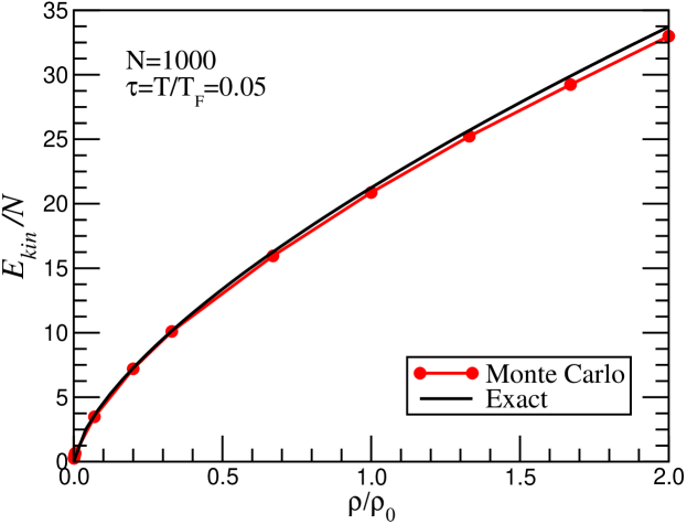
Figure 1: (color online) Average kinetic energy of a system of $N\!=\!1000$ identical fermions at a temperature of $\tau\!=\!T/T_{\rm F}\!=\!0.05$. The line with circles is the result of the Monte Carlo simulations with the Pauli potential of Eq. (18). The solid line is the exact behavior of a non-relativistic Fermi gas, as given by Eq. (10).

To our knowledge, reproducing the kinetic energy of a free Fermi gas is the sole constraint that has been imposed on most of the Pauli potentials available to date. However, while a host of Pauli potentials can reproduce such a behavior, it is unclear if these potentials can also reproduce the full momentum distribution. Thus, we now show how the Pauli potential defined in Eq. (18) is successful at reproducing two highly sensitive Fermi-gas observables, namely, the momentum distribution and the two-body correlation function.

III.2 Momentum Distribution

The momentum distribution obtained from the Monte-Carlo simulations is displayed in Fig. 2 for a variety of densities. Note that the momentum distribution has been normalized to one and that the densities have been expressed in units of $\rho_{0}\!=\!0.037~{}{\rm fm}^{-3}$. As indicated in Eq. (9), the momentum distribution of a cold Fermi gas depends solely on the two dimensionless ratios $q\!=\!p/p_{\rm F}$ and $\tau\!=\!T/T_{\rm F}$. Thus, all curves must collapse into the exact one — displayed by the (black) solid line — independent of density. It is gratifying to see that this is indeed the case. In contrast, we show in the next section that the standard Pauli potential of Eq. (16) fails to reproduce this behavior.

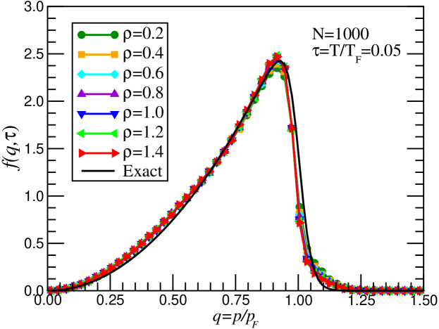
Figure 2: (color online) Momentum distribution of a system of $N\!=\!1000$ identical fermions at a temperature of $\tau\!=\!T/T_{\rm F}\!=\!0.05$ for a variety of densities (expressed in units of $\rho_{0}\!=\!0.037~{}{\rm fm}^{-3}$). The momentum distribution has been normalized to one [see Eq. (8)]. The (black) solid line with no symbols gives the exact behavior of a non-relativistic Fermi gas.

III.3 Two-Body Correlation Function

The two-body correlation function of a free Fermi gas is displayed in Fig. 3. The two-body correlation function $g(r)$ is related to the probability of finding two particles separated by a distance $r$. For a free Fermi gas, the probability of finding two identical fermions at zero separation is identically equal to zero [see Eq. (12)]. As this short-range (anti-)correlation is the sole consequence of the Pauli exclusion principle, the “Pauli hole” disappears for distances of the order of the interparticle separation ($p_{\rm F}^{-1}$). As in the case of the momentum distribution, the correlation function depends only on two dimensionless variables ($z\!=\!p_{\rm F}r$ and $\tau$). It is again gratifying that the simulation curves scale to the exact correlation function, depicted here with a (black) solid line.

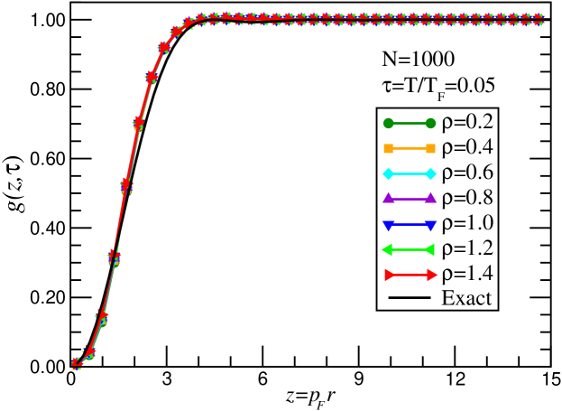
Figure 3: (color online) Two-body correlation function for a system of $N\!=\!1000$ identical fermions at a temperature of $\tau\!=\!T/T_{\rm F}\!=\!0.05$ for a variety of densities (expressed in units of $\rho_{0}\!=\!0.037~{}{\rm fm}^{-3}$). The (black) solid line with no symbols gives the exact behavior of a non-relativistic Fermi gas.

III.4 Comparison to other approaches

In this section we compare the Pauli potential introduced in Eq. (18) to earlier approaches that are based on Eq. (16). Such approaches have been very successful in reproducing the kinetic energy of a free Fermi gas for a wide range of densities. Indeed, the kinetic energy displayed in Fig. 2 of Ref. Maruyama et al. (1998) is as good — if not better — than the one obtained here.

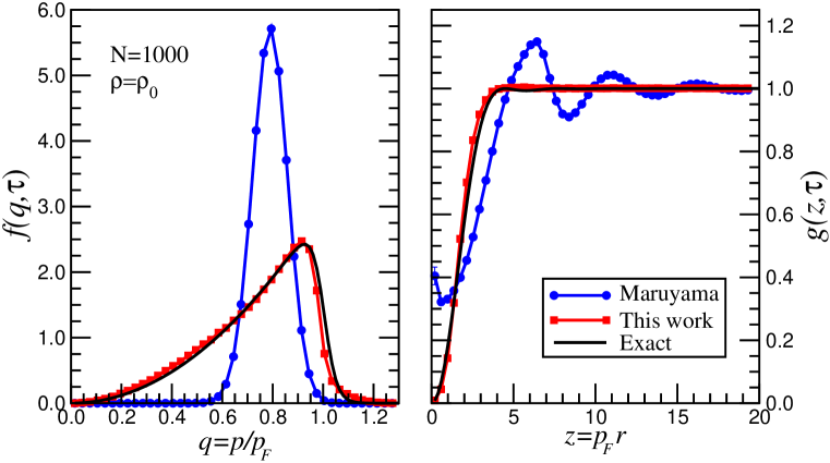
Figure 4: (color online) Comparison between the Pauli potential introduced in this work [Eq. (18)] and earlier approaches based on Eq. (16). The left-hand panel shows the momentum distribution while the right-hand panel the two-body correlation function. The simulations have been carried out for a system of $N\!=\!1000$ identical fermions at a density of $\rho_{0}\!=\!0.037~{}{\rm fm}^{-3}$. The (blue) line with circles is obtained from a Monte Carlo simulation using Eq. (16) with the parameters of Ref. Maruyama et al. (1998). The (red) line with squares displays the results using the Pauli potential introduced in this work; the black line gives the exact behavior of a non-relativistic Fermi gas.

However, a faithful reproduction of the kinetic energy does not guarantee that the system displays the same phase-space correlations as that of a free Fermi gas. To illustrate this point we compare in Fig. 4 the results from the two approaches for the momentum distribution and two-body correlation function at a fixed density of $\rho_{0}\!=\!0.037~{}{\rm fm}^{-3}$. The left-hand panel in the figure displays the momentum distribution and indicates that while earlier approaches (depicted with a blue line with circles) are accurate at reproducing the second moment of the distribution (i.e., the kinetic energy) the momentum distribution itself shows a behavior that differs significantly from that of a cold Fermi gas. The right-hand panel shows deficiencies that are as — or even more — severe. Two points are worth highlighting. First, the two-body correlation function $g(r)$ generated with the standard form of the Pauli potential does not vanish at $r\!=\!0$. Second, for distances of the order of the inter-particle separation and beyond, the two-body correlation function develops artificial oscillations. Failure in reproducing the correct behavior of $g(r)$ at $r\!=\!0$ is relatively simple to understand. Potentials based on Eq. (16) impose a penalty on the system only if both the positions and momenta of the two fermions are close to each other. Yet the correlations embodied in a free Fermi gas are significantly more stringent than that. Indeed, a Slater determinant vanishes if either the positions or the momenta of the two fermions are equal to each other. In contrast, the development of artificial structure in $g(r)$ is a more subtle effect that is intimately related to the momentum dependence of the potential and that we now address.

The artificial oscillations present in $g(r)$ are reminiscent of the structure of liquids and/or crystals. The emergence of crystalline structure in a low-temperature/low-density system would be expected if the energy of localization becomes small relative to the mutual repulsion between the particles. Such, however, is not the behavior of a cold Fermi gas. While spatial anti-correlations would favor the formation of a periodic structure, the large velocities of the particles — resulting from the Pauli exclusion principle — would make their localization extremely costly. What is not evident is the reason for the momentum distribution generated with a standard Pauli potential to lead to crystallization, whereas not that of a real Fermi gas (see left-hand panel in Fig. 4).

To our knowledge, the answer to this question was first provided by Neumann and Fai Neumann and Fai (1994). One must realize that any Hamiltonian that contains momentum-dependent interactions — such as most (if not all) Pauli potentials — generates a “canonical” momentum distribution that may (and does!) differ significantly from the corresponding “kinematical” momentum distribution $\langle{\bm{\pi}}\rangle\!\equiv\!\langle m\dot{{\bf r}}\rangle$. Indeed, in a Hamiltonian formalism where the Hamiltonian depends on the positions and canonical (not kinematical) momenta of all the particles, namely, $H=H({\bf p}_{1},\dots,{\bf p}_{N};{\bf r}_{1},\dots,{\bf r}_{N})$ the kinematical velocities must be obtained from Hamilton’s equations of motion, i.e., $\dot{\bf r}_{i}={\partial H}/\partial{\bf p}_{i}$. For a Hamiltonian that contains momentum-dependent interactions — as in the case of the Pauli potential — then the kinematical momentum ${\bm{\pi}}_{i}\!\equiv\!m\dot{{\bf r}}_{i}$ differs from the corresponding canonical momentum ${\bf p}_{i}$. This suggests that while a given choice of Pauli potential may produce the correct canonical momentum distribution, it may generate kinematical velocities that are too small to prevent crystallization. Such a distinction between canonical and kinematical momenta is an unwelcome, yet unavoidable, consequence of the approach. A cold Fermi gas — a system subjected to no interactions — is the quintessential quantum system were such an artificial distinction is not required.

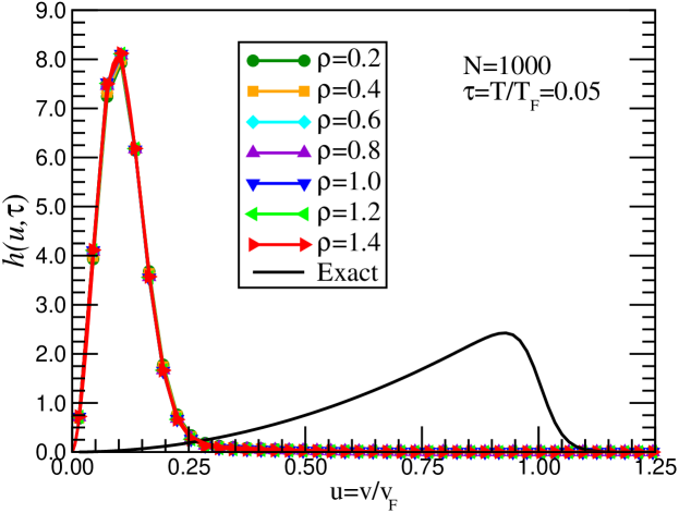
Figure 5: (color online) “Kinematical” velocity distribution of a system of $N\!=\!1000$ identical fermions at a temperature of $\tau\!=\!T/T_{\rm F}\!=\!0.05$ for a variety of densities (expressed in units of $\rho_{0}\!=\!0.037~{}{\rm fm}^{-3}$). The velocity distribution has been normalized to one. The (black) solid line with no symbols gives the exact behavior of a non-relativistic Fermi gas.

It is worth noting that although some earlier choices yield an extremely soft kinematical momentum distribution, the Pauli potential introduced in this work is not immune to such a disease. Indeed, we believe that an unrealistically soft kinematical momentum distribution is likely to be a general result of the Hamiltonian approach. Thus, we close this section by displaying in Fig. 5 the kinematical velocity distribution obtained with the new choice of Pauli potential introduced in Eq. (18). For comparison, the exact distribution of a cold Fermi gas (solid black line) is also included. The dependence of the Pauli potential on the canonical momentum distribution is responsible for generating such a soft velocity distribution, with its peak around 1/10 of the Fermi velocity. And while we were able to avoid crystallization with the present set of parameters (see Figs. 3 and 4), the risk of crystallization looms large (see next section).

III.5 Finite-Size Effects

We have observed that the Pauli potential introduced in Eq. (18), with its parameters suitably adjusted, has been successful in reproducing a variety of Fermi-gas observables, such as its kinetic energy, its (canonical) momentum distribution, and its two-body correlation function. However, the first indication of a potential problem — and one that may be generic to all approaches employing momentum-dependent interactions — is the emergence of an unrealistically soft velocity distribution and with it, the possibility of artificial spatial correlations (i.e., crystallization). Fortunately, with the choice of parameters adopted in this work, the problem of crystallization was avoided (see Fig. 3). Yet, there is no guarantee that crystallization will not become a problem as one examines the sensitivity of our results to finite-size effects.

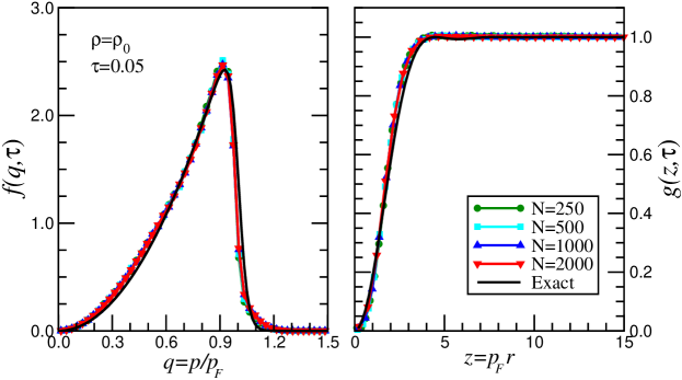
Figure 6: (color online) Finite-size effects on the canonical momentum distribution (left-hand panel) and the two-body correlation function (right-hand panel) for a system of identical fermions at a temperature of $\tau\!=\!T/T_{\rm F}\!=\!0.05$ and a density of $\rho=\!\rho_{0}\!=\!0.037~{}{\rm fm}^{-3}$. Simulations were carried out for systems containing $N\!=\!250,500,1000$ and $2000$ particles. The (black) solid line with no symbols gives the exact behavior of a non-relativistic Fermi gas.

In order to estimate the sensitivity of our results to finite-size effects, Monte Carlo simulations were performed for a system containing $N\!=\!250$, $N\!=\!500$, $N\!=\!1000$, and $N\!=\!2000$, identical fermions (note that the results reported so far have been limited to 1000 particles). The conclusions from this study are mixed. First (and fortunately) no evidence of crystallization or of significant finite-size effects were found. These findings are displayed in Fig. 6 for both the canonical momentum distribution (left-hand panel) and the two-body correlation function (right-hand) panel. Unfortunately, however, in order to preserve the high quality of the results previously obtained with 1000 particles, a parameter of the Pauli potential [$V_{B}^{0}$ in Eq. (18)] had to be fine tuned. Specifically, the following scaling with particle number was used:

$$V_{B}^{0}(N)=V_{B}^{0}(N\!=\!1000)\,\left(\frac{1000}{N}\right)\;,$$ (22)

with $V_{B}^{0}(N\!=\!1000)\!=\!1.26$ MeV being the value listed in Table 1. This unpalatable fact may be a reflection of the highly challenging task at hand: how to simulate fermionic many-body correlations by means of a “simple” two-body Pauli potential.

IV Conclusions

Semi-classical simulations of fermionic systems attempt to circumvent the many challenges posed by bona-fide quantum simulations through the inclusion of a fictitious Pauli potential Wilets et al. (1977); Dorso et al. (1987); Boal and Glosli (1988); Peilert et al. (1992); Maruyama et al. (1998); Watanabe et al. (2003). In the present contribution we conducted a critical study of the features and predictions of a widely used version of the Pauli potential. We concluded that the constraints imposed by such a Pauli potential, namely, the suppression of phase-space configurations having two fermions with both positions and momenta similar to each other, are too weak to faithfully reproduce some basic properties of a free Fermi gas. Instead, by examining the well-known behavior of the Slater determinant we suggest that phase-space configurations should be suppressed when either the positions or the momenta of the fermions are close to each other. By incorporating these features into a new form of the Pauli potential — and by carefully tuning the parameters of the model — the momentum distribution and the two-body correlation function of a free Fermi gas were accurately reproduced.

In the course of this study a pathology that is generic to all Pauli potential was uncovered. As pointed out by Neumann and Fai Neumann and Fai (1994) (to our knowledge for the first time), the “canonical” momentum distribution generated via Monte Carlo (or other) methods may differ significantly from the resulting “kinematical” momentum distribution. This suggests that while the kinetic energy of the free Fermi gas (computed from the canonical momenta) may be accurately reproduced, the distribution of velocities may be grossly distorted. Indeed, we found a distribution of velocities that significantly under-estimates — by a factor of 10 — that of a free Fermi gas. Such “sluggishness” among the particles could have disastrous consequences by inducing artificial ordering in the system (e.g., “crystallization”). The possible appearance of artificial long-range order in the system must be examined on a case by case basis. For example, with the standard version of the Pauli potential Maruyama et al. (1998) the system displays an anomalous two-body correlation function suggestive of crystallization. On the other hand, the Pauli potential introduced in this work faithfully reproduces the two-body correlation function of a free Fermi gas.

In conclusion a systematic study of the standard version of the Pauli potential has been conducted. While simple and widely used, such a version fails to reproduce some of the most basic properties of a free Fermi gas. Moreover, an analysis of the two-body correlation function generated by such a model reveals artificial long-range order. To correct these flaws a refined version of the Pauli potential was introduced. This new version — inspired by the properties of a Slater determinant — generated accurate (canonical) momentum distribution and two-body correlation functions, while avoiding crystallization. Yet the “kinematical” momentum distribution generated from such a Pauli potential was grossly underestimated. We believe this to be a generic feature of any momentum-dependent Pauli potential that is used in conjunction with a Hamiltonian approach Neumann and Fai (1994). Thus, the possibility for generating artificial correlations in the system (e.g., crystallization) looms large.

V ACKNOWLEDGMENTS

This work was supported in part by the United States Department of Energy grant DE- FG05-92ER40750 and by the Spanish Ministry of education under project DGI-FIS2006- 05319. One of the authors, M.A.P.G. would like to dedicate this work to the memory of J.M.L.G.

References

- Jamei et al. (2005) R. Jamei, S. Kivelson, and B. Spivak, Physical Review Letters 94, 056805 (2005).
- Horowitz et al. (2004a) C. J. Horowitz, M. A. Perez-Garcia, and J. Piekarewicz, Phys. Rev. C69, 045804 (2004a), eprint astro-ph/0401079.
- Horowitz et al. (2004b) C. J. Horowitz, M. A. Perez-Garcia, J. Carriere, D. K. Berry, and J. Piekarewicz, Phys. Rev. C70, 065806 (2004b), eprint astro-ph/0409296.
- Horowitz et al. (2005) C. J. Horowitz, M. A. Perez-Garcia, D. K. Berry, and J. Piekarewicz, Phys. Rev. C72, 035801 (2005), eprint nucl-th/0508044.
- Grotendorst et al. (2002) J. Grotendorst, D. Marx, and A. Muramatsu, eds., Quantum Simulations of Complex Many-Body Systems: From Theory to Algorithms, Lecture Notes (John von Neumann-Institut für Computing (NIC), The Netherlands, 2002).
- Wilets et al. (1977) L. Wilets, E. M. Henley, M. Kraft, and A. D. MacKellar, Nucl. Phys. A282, 341 (1977).
- Dorso et al. (1987) C. Dorso, S. Duarte, and J.Randrup, Phys. Lett. B 188, 287 (1987).
- Boal and Glosli (1988) D. H. Boal and J. N. Glosli, Phys. Rev. C 38, 1870 (1988).
- Peilert et al. (1992) G. Peilert, J. Konopka, H. Stöcker, W. Greiner, M. Blann, and M. G. Mustafa, Phys. Rev. C 46, 1457 (1992).
- Maruyama et al. (1998) T. Maruyama et al., Phys. Rev. C57, 655 (1998), eprint nucl-th/9705039.
- Watanabe et al. (2003) G. Watanabe, K. Sato, K. Yasuoka, and T. Ebisuzaki, Phys. Rev. C 68, 035806 (2003).
- Pathria (1996) R. K. Pathria, Statistical Mechanics (Butterworth-Heinemann, Oxford, 1996), 2nd ed.
- Fetter and Walecka (1971) A. L. Fetter and J. D. Walecka, Quantum Theory of Many Particle Systems (McGraw-Hill, New York, 1971).
- Vesely (2001) F. J. Vesely, Computational Physics: An Introduction (Kluwer Academic, New York, 2001).
- Neumann and Fai (1994) J. J. Neumann and G. I. Fai, Phys. Lett. B329, 419 (1994), eprint nucl-th/9404025.