Spectra and Symmetry in Nuclear Pairing

Abstract

We apply the algebraic Bethe ansatz technique to the nuclear pairing problem with orbit dependent coupling constants and degenerate single particle energy levels. We find the exact energies and eigenstates. We show that for a given shell, there are degeneracies between the states corresponding to less and more than half full shell. We also provide a technique to solve the equations of Bethe ansatz.

I Introduction

Pairing is known to play an important role in the quantum many-body problems. In particular, pairing force is a key ingredient of the residual interaction between nucleons in a nucleus. An algebraic approach to pairing was given by Richardson some time ago rich . Richardson’s formalism was rather complex and was not widely used in nuclear physics. For a limited class of seniority-conserving pairing interactions, the quasispin formalism of Kerman kerman1 was used to treat a large number of cases. In this article, we wish to explore an approach related to Richardson’s formalism which can be reduced to the quasispin formalism in the appropriate limit.

In the nuclear shell model, the nucleus is pictured as a system of fermions moving in a central field with well defined single particle energy levels $\epsilon_{j}$, arising from spin-orbit interactions. We consider nucleons at time-reversed states $|j\>m\rangle$ and $(-1)^{(j-m)}|j\>-m\rangle$, interacting with a pairing force described by the Hamiltonian

$$\hat{H}=\sum_{jm}\epsilon_{j}a^{\dagger}_{j\>m}a_{j\>m}-|G|\sum_{jj^{\prime}}c_{jj^{\prime}}\hat{S}^{+}_{j}\hat{S}^{-}_{j^{\prime}}.$$ (1)

Here, $a^{\dagger}_{j\>m}$ and $a_{j\>m}$ are the creation and annihilation operators for nucleons in level $j$, respectively, and $c_{jj^{\prime}}$ is the strength of the pairing interaction between levels $j$ and $j^{\prime}$. The quasispin operators $\hat{S}^{+}_{j}$ and $\hat{S}^{-}_{j}$ are given by

$$\hat{S}^{+}_{j} = \sum_{m>0}(-1)^{(j-m)}a^{\dagger}_{j\>m}a^{\dagger}_{j\>-m},$$ (2)

$$\hat{S}^{-}_{j} = \sum_{m>0}(-1)^{(j-m)}a_{j\>-m}a_{j\>m}.$$

These operators create or destroy a single pair of nucleons in the time reversed states on level $j$. If we also define

$$\hat{S}^{0}_{j}=\frac{1}{2}\sum_{m>0}\left(a^{\dagger}_{j\>m}a_{j\>m}+a^{\dagger}_{j\>-m}a_{j\>-m}-1\right),$$ (3)

together with the operators in Eqs. (2) we have a set of orthogonal $SU(2)$ algebras

$$[\hat{S}^{+}_{j},\hat{S}^{-}_{j^{\prime}}]=2\delta_{jj^{\prime}}\hat{S}^{0}_{j}\ \ \ \ \ \ [\hat{S}^{0}_{j},\hat{S}^{\pm}_{j^{\prime}}]=\pm\delta_{jj^{\prime}}\hat{S}^{\pm}_{j}.$$ (4)

Note that $\hat{S}^{0}_{j}$ can also be written as

$$\hat{S}^{0}_{j}=\hat{N}_{j}-\frac{1}{2}\Omega_{j}.$$ (5)

Here $\Omega_{j}=j+\frac{1}{2}$ is the maximum number of pairs that can occupy level $j$ and $\hat{N}_{j}$ is the pair number operator level $j$ which is given by

$$\hat{N}_{j}=\frac{1}{2}\sum_{m>0}\left(a^{\dagger}_{j\>m}a_{j\>m}+a^{\dagger}_{j\>-m}a_{j\>-m}\right).$$ (6)

$\hat{N}_{j}$ takes values from zero to $\Omega_{j}$ and thus $\hat{S}^{0}_{j}$ takes values from $-\frac{1}{2}\Omega_{j}$ to $\frac{1}{2}\Omega_{j}$. Consequently, the $SU(2)$ spanned by $\hat{S}^{\pm}_{j}$ and $\hat{S}^{0}_{j}$ live in the spin $\frac{1}{2}\Omega_{j}$ representation.

When the pairing strength is separable ($c_{jj^{\prime}}=c^{*}_{j}c_{j^{\prime}}$), the Hamiltonian given in Eq. (1) takes the form

$$\hat{H}=\sum_{jm}\epsilon_{j}a^{\dagger}_{j\>m}a_{j\>m}-|G|\sum_{jj^{\prime}}c^{*}_{j}c_{j^{\prime}}\hat{S}^{+}_{j}\hat{S}^{-}_{j^{\prime}}.$$ (7)

Furthermore, if we assume that the energy levels are degenerate, the first term is a constant for a given number of pairs because the Hamiltonian is number conserving. Ignoring this term, we obtain

$$\hat{H}=-|G|\sum_{jj^{\prime}}c^{*}_{j}c_{j^{\prime}}\hat{S}^{+}_{j}\hat{S}^{-}_{j^{\prime}}.$$ (8)

Defining the operators

$$\hat{S}^{+}(0)=\sum_{j}c^{*}_{j}\hat{S}^{+}_{j}\ \ \ \ \mbox{and}\ \ \ \ \ \hat{S}^{-}(0)=\sum_{j}c_{j}\hat{S}^{-}_{j},$$ (9)

the Hamiltonian in Eq. (8) can be written as

$$\hat{H}=-|G|\hat{S}^{+}(0)\hat{S}^{-}(0).$$ (10)

The reason that we choose to label the operators in Eq. (9) as $\hat{S}^{\pm}(0)$ will become clear in what follows. Physically, the operator $\hat{S}^{+}(0)$ creates a single fermion pair and $c^{*}_{j}$ can be viewed as the probability amplitude that this pair is created at level $j$. This interpretation implies, however, that these constants are normalized:

$$\sum_{j}|c_{j}|^{2}=1.$$ (11)

Note that a state with no pairs, here denoted by $|0\rangle$, is the lowest weight state for all the $SU(2)$ algebras corresponding to different levels. In other words, it obeys

$$\hat{S}^{-}_{j}|0\rangle=0\ \ \ \mbox{and}\ \ \ \hat{S}^{0}_{j}|0\rangle=-\frac{\Omega_{j}}{2}|0\rangle\ \ \ \ \mbox{for every $j$}.$$ (12)

Therefore, this state is annihilated by the Hamiltonian in Eq. (8)

$$\hat{H}|0\rangle=0.$$ (13)

The state which represents the full shell, denoted by $|\bar{0}\rangle$ in this paper, is the highest weight state of all $SU(2)$ algebras corresponding to different levels. It obeys

$$\hat{S}^{+}_{j}|\bar{0}\rangle=0\ \ \ \mbox{and}\ \ \ \hat{S}^{0}_{j}|\bar{0}\rangle=\frac{\Omega_{j}}{2}|\bar{0}\rangle\ \ \ \ \mbox{for every $j$}.$$ (14)

The state $|\bar{0}\rangle$ is also an eigenstate of the Hamiltonian

$$\hat{H}|\bar{0}\rangle=E_{1}|\bar{0}\rangle.$$ (15)

Its energy is given by

$$E_{1}=-|G|\sum_{j}\Omega_{j}|c_{j}|^{2}.$$ (16)

Unlike the fully occupied or empty shell, it is considerably more difficult to calculate the eigenstates and the energies when the shell is partially occupied. In a study of states with generalized seniority zero, Talmi talmi considered states of two particles coupled to angular momentum zero. He showed that under certain assumptions, a state of the form

$$\hat{S}^{+}(0)|0\rangle=\sum_{j}c^{*}_{j}\hat{S}^{+}_{j}|0\rangle$$ (17)

is an eigenstate of a class of Hamiltonians including that in Eq. (8). It is fairly straightforward to show that the Hamiltonian in Eq. (8) satisfies

$$\hat{H}\hat{S}^{+}(0)|0\rangle=E_{1}\hat{S}^{+}(0)|0\rangle$$ (18)

where $E_{1}$ is given by Eq. (16). We see that the state in Eq. (17) which has one pair of nucleons has the same energy as the full shell state $|\bar{0}\rangle$. Obviously, the state given in Eq. (17) is not the only eigenstate for one pair of nucleons. For example, for two levels with total angular momenta $j_{1}$ and $j_{2}$, it is straightforward to show that the state

$$\left(\frac{c_{j_{2}}}{\Omega_{j_{1}}}\hat{S}^{+}_{j_{1}}-\frac{c_{j_{1}}}{\Omega_{j_{2}}}\hat{S}^{+}_{j_{2}}\right)|0\rangle,$$ (19)

which is orthogonal to the state (17), is also an eigenstate of the Hamiltonian in Eq. (8).

One may ask if there is a systematic way to derive these states. The authors of Ref. Pan:1997rw came up with an elegant solution to this question. They calculated the energy eigenvalues and eigenstates of the Hamiltonian given in Eq. (8) using the operators

$$\hat{S}^{+}(x)=\sum_{j}\frac{c^{*}_{j}}{1-|c_{j}|^{2}x}\hat{S}^{+}_{j}\ \ \ \ \ \mbox{and}\ \ \ \ \ \hat{S}^{-}(x)=\sum_{j}\frac{c_{j}}{1-|c_{j}|^{2}x}\hat{S}^{-}_{j}.$$ (20)

Here, $x$ is a parameter which can be real or complex. In this technique, one starts from the empty shell $|0\rangle$ and constructs Bethe ansatz states using the operators $S^{+}(x)$. Substitution of these states into the energy equation yields Bethe ansatz equations (BAE) which determine the values of the parameters $x$. Note that the operators given in Eq. (9) are special cases of the operators defined in Eq. (20) for $x=0$. The authors of Ref. Pan:1997rw successfully adopted the procedure outlined above and obtained the energy eigenstates and eigenvalues of the Hamiltonian given in Eq. (8). Their proof, however, relies on a Laurent expansion of the operators $\hat{S}^{\pm}(x)$ around $x=0$. Later, they use an analytic continuation argument to vindicate the validity of their results in the entire complex plane except some singular points.

In this paper, we give an alternative, algebraic proof which does not impose the analyticity condition and valid in general for any complex values of the constants $c_{j}$. We also show that the same technique works for the pairs of holes. In other words, the Bethe ansatz states can be constructed with the operators $S^{-}(x)$ acting the fully occupied shell $|\bar{0}\rangle$. As we will show, one obtains the same Bethe ansatz equations and the same energies for states with $N$ nucleon pairs and $N-1$ hole pairs (which is equivalent to $N_{max}+1-N$ particle pairs). Here $N_{max}$ is the maximum number of pairs that can occupy the shell in question and $N\leq N_{max}/2$. The symmetry between the states $|\bar{0}\rangle$ and $\hat{S}^{+}(0)|0\rangle$ pointed out in Eqs. (15) and (18) is a special case of this symmetry for $N=1$.

Here, we also provide techniques for solving the resulting Bethe ansatz equations. One should point out that it is also possible to solve the pairing problem numerically in the quasispin basis Volya:2000ne . Our approach is complementary to this numerical approach.

This paper is organized as follows: In Section II, we outline the Bethe ansatz formalism and give the eigenstates and eigenvalues of the pairing Hamiltonian. In this section, we also compare our results with the quasispin limit of the problem. In Section III, we consider the special case of a shell with two levels. We show that, the problem of solving the equations of Bethe ansatz with two levels for zero energy eigenstates can be transformed into a problem of finding the roots of an hypergeometric polynomial. In Section IV, we compare our results with the available data in the literature. We present our conclusions in Section V.

II Eigenstates and Eigenvalues of the Nuclear Pairing Hamiltonian

We begin by introducing the operator

$$\hat{K}^{0}(x)=\sum_{j}\frac{1}{1/|c_{j}|^{2}-x}\hat{S}_{j}^{0}$$ (21)

in addition to the operators in Eq. (20). It is straightforward to show that the following commutators are satisfied by $\hat{S}^{+}(x)$, $\hat{S}^{-}(x)$ and $\hat{K}^{0}(x)$:

$$[\hat{S}^{+}(x),\hat{S}^{-}(0)] = [\hat{S}^{+}(0),\hat{S}^{-}(x)]=2K^{0}(x),$$ (22)

$$[\hat{K}^{0}(x),\hat{S}^{\pm}(y)] = \pm\frac{\hat{S}^{\pm}(x)-\hat{S}^{\pm}(y)}{x-y}.$$ (23)

When $x=y$, the limit has to be taken on both sides of Eq. (23) as $y\to x$. The states $|0\rangle$ and $|\bar{0}\rangle$ defined with Eqs. (12) and (14), respectively, are eigenstates of $\hat{K}^{0}(x)$:

$$\hat{K}^{0}(x)|0\rangle=-\left(\sum_{j}\frac{\Omega_{j}/2}{1/|c_{j}|^{2}-x}\right)|0\rangle,\ \ \ \ \ \ \ \hat{K}^{0}(x)|\bar{0}\rangle=\left(\sum_{j}\frac{\Omega_{j}/2}{1/|c_{j}|^{2}-x}\right)|\bar{0}\rangle.$$ (24)

Below, we construct the eigenstates of the Hamiltonian $\hat{H}$ using the algebraic Bethe ansatz formalism. We first consider the eigenstates with one pair of nucleons in order to demonstrate the technique. Then we discuss the general case with more than one pair.

II.1 Eigenstates With One Pair of Nucleons

Let us first form a Bethe ansatz state as follows:

$$\hat{S}^{+}(x^{(1)})|0\rangle.$$ (25)

We denoted our variable by $x^{(1)}$ in order to emphasize that this state has one pair of nucleons. Using the form of the Hamiltonian given in Eq. (10), together with Eq. (13) and Eqs. (22)-(24), we can show that the Hamiltonian acting on this state gives

$$\hat{H}\hat{S}^{+}(x^{(1)})|0\rangle=-2|G|\left(\sum_{j}\frac{\Omega_{j}/2}{1/|c_{j}|^{2}-x^{(1)}}\right)\hat{S}^{+}(0)|0\rangle.$$ (26)

Setting $x^{(1)}=0$ in the state (25), one obtains the state in Eq. (17). One can see from Eq. (26) that the corresponding energy is as in Eq. (16).

Alternatively, we can choose $x^{(1)}$ as a solution of

$$\sum_{j}\frac{-\Omega_{j}/2}{1/|c_{j}|^{2}-x^{(1)}}=0.$$ (27)

Then Eq. (26) becomes

$$\hat{H}\hat{S}^{+}(x^{(1)})|0\rangle=0.$$ (28)

In other words, for the values of $x^{(1)}$ satisfying Eq. (27), the state given in Eq. (25) is an eigenstate of $\hat{H}$ with zero energy. Here Eq. (27) is our one-pair Bethe ansatz equation because it determines the value of $x^{(1)}$.

The eigenstates with one pair of nucleons discussed here can also be seen in Table 1. We see that when there is only one pair of nucleons occupying the shell, the Hamiltonian $\hat{H}$ of Eq. (8) has only one eigenstate with nonzero energy which is $\hat{S}^{+}(0)|0\rangle$. All other eigenstates are orthogonal to this state and have zero energy. In fact, the BAE (27) can be seen as this orthogonality relation. In many cases, the BAE in Eq. (27) has more than one solution and each solution gives us an eigenstate in the form of Eq. (25) with zero energy. As discussed in Section III, in the presence of two levels, Eq. (27) has only one solution and this solution gives the state (19). In the presence of, for example, three levels, Eq. (27) has two distinct solutions and therefore we have two zero energy states. These states can be seen in Table 5.

II.2 Eigenstates With More Than One Pair of Nucleons

The eigenstates of the Hamiltonian in Eq. (8) with more than one nucleon pair can also be written in the Bethe ansatz. Some of these states have zero energy, like the state in Eq. (25), and some of them have nonzero energy, like the state in Eq. (17). We examine these states below and the results of this section are summarized in Table 1.

# of pairs	Bethe Ansatz Equations	State	Energy$/\left(-|G|\right)$
Less than half full or half full shell
$1$	$\displaystyle\sum_{j}\frac{-\Omega_{j}/2}{1/|c_{j}|^{2}-x^{(1)}}=0$	$\displaystyle\hat{S}^{+}(x^{(1)})|0\rangle$	0
	No BAE	$\displaystyle\hat{S}^{+}(0)|0\rangle$	$\displaystyle\sum_{j}\Omega_{j}|c_{j}|^{2}$
$N$	$\displaystyle\sum_{j}\frac{-\Omega_{j}/2}{1/c_{j}^{2}-x^{(N)}_{m}}=\sum_{k=1(k\neq m)}^{N}\frac{1}{x^{(N)}_{m}-x^{(N)}_{k}}$	$\displaystyle\hat{S}^{+}(x^{(N)}_{1})\hat{S}^{+}(x^{(N)}_{2})\dots\hat{S}^{+}(x^{(N)}_{N})|0\rangle$	0
	For $m=1,2,\dots,N$
	$\displaystyle\sum_{j}\frac{-\Omega_{j}/2}{1/|c_{j}|^{2}-z^{(N)}_{m}}=\frac{1}{z^{(N)}_{m}}+\sum_{k=1(k\neq m)}^{N-1}\frac{1}{z^{(N)}_{m}-z^{(N)}_{k}}$	$\displaystyle\hat{S}^{+}(0)\hat{S}^{+}(z^{(N)}_{1})\dots\hat{S}^{+}(z^{(N)}_{N-1})|0\rangle$	$\displaystyle\sum_{j}\Omega_{j}|c_{j}|^{2}-\sum_{k=1}^{N-1}\frac{2}{z^{(N)}_{k}}$
	For $m=1,2,\dots,N-1$
More than half full shell
$\displaystyle N_{max}+1-N$	$\displaystyle\sum_{j}\frac{-\Omega_{j}/2}{1/|c_{j}|^{2}-z^{(N)}_{m}}=\frac{1}{z^{(N)}_{m}}+\sum_{k=1(k\neq m)}^{N-1}\frac{1}{z^{(N)}_{m}-z^{(N)}_{k}}$	$\displaystyle\hat{S}^{-}(z_{1}^{(N)})\hat{S}^{-}(z_{2}^{(N)})\dots\hat{S}^{-}(z_{N-1}^{(N)})|\bar{0}\rangle$	$\displaystyle\sum_{j}\Omega_{j}|c_{j}|^{2}-\sum_{k=1}^{N-1}\frac{2}{z^{(N)}_{k}}$
	For $m=1,2,\dots,N-1$
$\displaystyle N_{max}$	No BAE	$\displaystyle|\bar{0}\rangle$	$\displaystyle\sum_{j}\Omega_{j}|c_{j}|^{2}$

Table 1: Summary of the energy eigenvalues and the eigenstates of the pairing Hamiltonian. Here, $N_{max}$ denotes the maximum number of pairs which can occupy the shell and $\displaystyle 2\leq N\leq N_{max}/2$. For shells which are at most half full, $N$ corresponds to the number of pairs as can be seen in the upper part of the first column. For shells which are more than half full, $N$ is related to the number of pairs as indicated in the lower part of the first column. Note that for more than half full shells there are no zero energy states.

II.2.1 The Eigenstates With Non-zero Energy

Using the form of the Hamiltonian given in Eq. (10), together with Eq. (13) and (22)-(24), it is possible to show that the state

$$\hat{S}^{+}(0)\hat{S}^{+}(z^{(N)}_{1})\dots\hat{S}^{+}(z^{(N)}_{N-1})|0\rangle$$ (29)

is an eigenstate of the Hamiltonian if the parameters $z^{(N)}_{k}$ obey the following Bethe ansatz equations (see the Appendix)

$$\sum_{j}\frac{-\Omega_{j}/2}{1/|c_{j}|^{2}-z^{(N)}_{m}}=\frac{1}{z^{(N)}_{m}}+\sum_{k=1(k\neq m)}^{N-1}\frac{1}{z^{(N)}_{m}-z^{(N)}_{k}},\ \ \ \ \ \ \mbox{for every}\ \ m=1,2,\dots N-1.$$ (30)

The state in Eq. (29) has $N$ pairs of nucleons and this is the reason we use the superscript $(N)$. Here, we are assuming that $2\leq N\leq N_{max}/2$. The case for one nucleon is already examined in Section II.A and if the shell is more than half full, we choose to work with hole pairs instead of particle pairs. Therefore the state (30) represents a shell which is at most half full. The details of this calculation can be found in the Appendix. Here, we would like to emphasize that the BAE’s (30) are a set of $N-1$ coupled equations in $N-1$ variables. The parameters $z^{(N)}_{m}$ are all different from one another and they are also different from zero.

Using the same parameters $z^{(N)}_{m}$ that appear in Eq. (29), we now form the state

$$\hat{S}^{-}(z_{1}^{(N)})\hat{S}^{-}(z_{2}^{(N)})\dots\hat{S}^{-}(z_{N-1}^{(N)})|\bar{0}\rangle.$$ (31)

This state has $N_{max}+1-N$ pairs of nucleons because it starts from the full shell with $N_{max}$ pairs of nucleons, represented by $|\bar{0}\rangle$ and then destroys $N-1$ pairs. Since we assumed that $2\leq N\leq N_{max}/2$, this state represents a shell which is more than half full. In the Appendix, we show that if the parameters $z^{(N)}_{k}$ obey the equations of Bethe ansatz given in Eqs. (30), then the state (31) is also an eigenstate of the Hamiltonian like the state (29). We can also show that the states (29) and (31) have the same energy which is given in terms of the variables $z^{(N)}_{k}$ as follows:

$$E_{N}=-|G|\left(\sum_{j}\Omega_{j}|c_{j}|^{2}-\sum_{k=1}^{N-1}\frac{2}{z^{(N)}_{k}}\right).$$ (32)

At this point, we would like to remark that the solutions of the BAE given in Eqs. (30) may be complex. Nevertheless, since the complex solutions always come in conjugate pairs, the energy in Eq. (32) is always real.

In principle, Eqs. (30) may have more than one solution in which case each solution gives us two eigenstates. One should substitute each solution in Eqs. (29) and (31) in order to find corresponding eigenstates and then in Eq. (32) in order to find their energy.

The state in Eq. (29) can be thought as the generalization of the state in Eq. (17) found by Talmi talmi . For $N=2$, the state (29) becomes

$$\hat{S}^{+}(0)\hat{S}^{+}(z^{(2)}_{1})|0\rangle$$ (33)

and the state (31) becomes

$$\hat{S}^{-}(z^{(2)}_{1})|\bar{0}\rangle.$$ (34)

The state in Eq. (33) has $2$ nucleon pairs whereas the state in Eq. (34) has $N_{max}-1$ nucleon pairs. We have only one unknown variable, $z^{(2)}_{1}$, and the BAE we must solve to determine it can be found by substituting $N=2$ in Eqs. (30). Note that the sum in the last term of Eqs. (30) does not contain any terms for $N=2$ so that the Bethe ansatz equation is

$$\sum_{j}\frac{-\Omega_{j}/2}{1/|c_{j}|^{2}-z^{(2)}_{1}}=\frac{1}{z^{(2)}_{1}}.$$ (35)

From Eq. (32), we find the energy of the states in Eqs. (33) and (34) to be

$$E_{2}=-|G|\left(\sum_{j}\Omega_{j}|c_{j}|^{2}-\frac{2}{z^{(2)}_{1}}\right).$$ (36)

By solving Eq. (35), one determines the values of $z^{(2)}_{1}$ and then substitutes each solution in the states in Eqs. (33) and (34) in order to find the corresponding eigenstates and then in Eq. (36) in order to find the energies of these states.

We would like to note that although we call the states in Eqs. (29) and (31) nonzero energy states, in principle, the energy calculated from Eq. (32) may turn out to be zero for some specific values of the parameters $\Omega_{j}$ and $c_{j}$. Nevertheless, for generic values of the parameters of the problem, the energies of the states described here are different from zero as opposed to the states we examine below which are annihilated by the Hamiltonian and therefore have identically zero energy.

II.2.2 The Eigenstates with Zero Energy

In the Appendix, we show that a state of the form

$$\hat{S}^{+}(x^{(N)}_{1})\hat{S}^{+}(x^{(N)}_{2})\dots\hat{S}^{+}(x^{(N)}_{N})|0\rangle$$ (37)

is annihilated by the Hamiltonian $\hat{H}$ of Eq. (8), if the parameters $x^{(N)}_{k}$ satisfy the following Bethe ansatz equations:

$$\sum_{j}\frac{-\Omega_{j}/2}{1/|c_{j}|^{2}-x^{(N)}_{m}}=\sum_{k=1(k\neq m)}^{N}\frac{1}{x^{(N)}_{m}-x^{(N)}_{k}},\ \ \ \ \ \ \mbox{for every}\ \ \ m=1,2,\dots,N.$$ (38)

The state in Eq. (37) has $N$ nucleon pairs where $2\leq N\leq N_{max}/2$. Here, the parameters $x^{(N)}_{k}$ may be real or complex, but they are all different from one another.

We would like to emphasize that the Bethe ansatz equations (38) may have more than one solution. In this case, each solution gives us an eigenstate in the form of Eq. (37) with zero energy. It may also be the case that the BAE in Eqs. (38) do not admit any solutions for some $N$. This is not surprising given the fact that it may not always be possible to find a zero energy configuration for any number of pairs.

II.3 Quasispin Limit

The results obtained in Sections II.A and II.B reveal a symmetry between the nonzero energy spectra of the pairing Hamiltonian with $N$ pairs and $N_{max}+1-N$ pairs of nucleons. Here $N_{max}$ is the total number of pairs that can occupy the shell and $N\leq N_{max}/2$. This means that for a given shell, there are degeneracies between the eigenstates of the nuclei corresponding to less and more than half full shell. Here we examine the quasispin limit of the problem to gain insight about this symmetry. We also show that zero energy states do not obey this symmetry because there are no zero energy states for the nuclei corresponding to more than half full shell.

Let us consider a shell consisting of $d$ levels $j_{1}$, $j_{2}$, $\dots$, $j_{d}$ with maximum occupancies $\Omega_{j_{1}}$, $\Omega_{j_{2}}$, $\dots$, $\Omega_{j_{d}}$. If we assume that the occupation amplitudes for these levels are all equal to one another, i.e., $c_{j_{1}}=c_{j_{2}}=\dots=c_{j_{d}}$, then the pairing Hamiltonian of Eq. (8) is proportional to

$$Q^{+}Q^{-}=\overrightarrow{Q}\cdot\overrightarrow{Q}-Q^{0}\left(Q^{0}-1\right)$$ (39)

where

$$\overrightarrow{Q}=\overrightarrow{S}_{j_{1}}+\overrightarrow{S}_{j_{2}}+\dots+\overrightarrow{S}_{j_{d}}$$ (40)

is the sum of the quasispins corresponding to different levels. Since the quasispin quantum number corresponding to level $j$ is $\Omega_{j}$, Eq. (40) corresponds to the addition of the angular momenta $\Omega_{j_{1}}/2$, $\Omega_{j_{2}}/2$, $\dots$, $\Omega_{j_{d}}/2$. In this limit, the eigenstates of the pairing Hamiltonian are $|J\>M\rangle$, where $J$ is the total angular momentum. The energies are given by

$$Q^{+}Q^{-}|J\>M\rangle=\left[J(J+1)-M(M-1)\right]|J\>M\rangle.$$ (41)

Clearly, the lowest weight states $|J\>-J\rangle$ have zero energy. These are the quasispin limit of the zero energy states given in Eq. (37). The other states which have nonzero energies can be written as $|J\>\tilde{M}\rangle$ and $|J\>1-\tilde{M}\rangle$ if we define $-J+1\leq\tilde{M}\leq 0$. These states are the quasispin limit of the states given in Eqs. (29) and (31), respectively. To see this, first note that from Eq. (5) we find

$$Q^{0}=\sum_{j}\hat{S}^{0}_{j}=\hat{N}_{tot}-\frac{N_{max}}{2}$$ (42)

where $\hat{N}_{tot}$ is the total pair number operator. We can use this equation to find the number of pairs in a state $|J\>M\rangle$ as

$$\hat{N}_{tot}|J\>M\rangle=\left(M+\frac{N_{max}}{2}\right)|J\>M\rangle.$$ (43)

This equation tells us that if the state $|J\>\tilde{M}\rangle$ has $N$ pairs of nucleons, then the state $|J\>1-\tilde{M}\rangle$ has $N_{max}+1-N$ pairs of nucleons where $N\leq N_{max}/2$. We also see from Eq. (41) that the states $|J\>\tilde{M}\rangle$ and $|J\>1-\tilde{M}\rangle$ have the same energy. This is consistent with the results found above, i.e., that the nonzero energy eigenstates of the pairing Hamiltonian with $N$ pairs and $N_{max}+1-N$ pairs have the same energy. Although this symmetry is trivial in the quasispin limit, we have proved that it is valid for generic values of occupation amplitudes $c_{j}$ as well.

The quasispin limit of the problem also tells us about the zero energy states of the pairing Hamiltonian for a given number of pairs. In general, it is difficult to tell if a zero energy configuration exists for a given number of pairs just by looking at the equations of Bethe ansatz (38). These equations are not always guaranteed to have solutions leading to nontrivial states. Nevertheless, Eq. (10) tells us that the zero energy states of the pairing Hamiltonian are the states annihilated by $\hat{S}^{-}(0)$ defined in Eq. (9). In the quasispin limit, $\hat{S}^{-}(0)$ is proportional to $Q^{-}$ and the zero energy states become the lowest weight states $|J\>-J\rangle$. Therefore, we can restrict ourselves to the quasispin limit as long as the discussion is limited to the existence of zero energy states of the pairing Hamiltonian with a given number of pairs. In this case, Eq. (43) tells us that the number of pairs in a zero energy state $|J\>-J\rangle$ is $N_{max}/2-J$. Since $J\geq 0$, we conclude that zero energy states do not exist for a more than half full shell.

In many cases, we can come to an even stronger conclusion on the existence of the zero energy states by examining the quasispin limit. For example, in the presence of two levels $j_{1}$ and $j_{2}$, quasispin limit corresponds to the addition of the two angular momenta $\Omega_{j_{1}}/2$ and $\Omega_{j_{2}}/2$. Assuming that $\Omega_{j_{2}}>\Omega_{j_{1}}$, the sum of the two angular momenta yields the following set of orthogonal representations:

$$J=\frac{\Omega_{j_{2}}+\Omega_{j_{1}}}{2},\frac{\Omega_{j_{1}}+\Omega_{j_{2}}}{2}-1,\frac{\Omega_{j_{1}}+\Omega_{j_{2}}}{2}-2\dots,\frac{\Omega_{j_{2}}-\Omega_{j_{1}}}{2}.$$ (44)

We have a zero energy state $|J\>-J\rangle$ for each one of them. From Eq. (43) we see that the lowest weight state $|J\>-J\rangle$ has $N_{max}/2-J$ nucleon pairs. In this special case $N_{max}=\Omega_{j_{2}}+\Omega_{j_{1}}$. Using this, we find that the zero energy states exists only for $N=0,1,2,\dots,\Omega_{j_{1}}$. Since we set $\Omega_{1}$ as the smaller of $\Omega_{1}$ and $\Omega_{2}$ and since there is no degeneracy in Eq. (44), we conclude that, in the presence of two levels, one and only one zero energy state exists for each number of pairs until there are enough pairs to fill one of the levels. After that, no zero energy state exists.

III Exact Solution for Two Nuclear Energy Levels

In the previous section, we showed that in a system of two nuclear levels, zero energy states of the pairing Hamiltonian exist only for small number of pairs, i.e., when the number of pairs is not more than enough to fill any one of the levels. Here, we consider the Bethe ansatz equations which are to be solved in order to find the states annihilated by the pairing Hamiltonian (i.e. Eqs. (27) and (38)) for two levels and for arbitrary values of the occupation probabilities $|c_{j_{1}}|^{2}$ and $|c_{j_{1}}|^{2}$. We give analytical solutions of these equations in the form of the roots of some hypergeometric polynomials. The method we use here is adopted from Ref. Balantekin:2004yf .

The Bethe ansatz equations for states annihilated by $\hat{H}$ were given by Eq. (27) for pair of nucleons and by Eqs. (38) for more than one pair of nucleons. When there are only two levels, these equations can be written as

$$\frac{-\Omega_{j_{1}}/2}{1/|c_{j_{1}}|^{2}-x_{i}^{(N)}}+\frac{-\Omega_{j_{2}}/2}{1/|c_{j_{2}}|^{2}-x_{i}^{(N)}}=\sum_{k=1(k\neq i)}^{N}\frac{1}{x_{i}^{(N)}-x_{k}^{(N)}},$$ (45)

for $i=1,2,\dots,N$. These equations are to be satisfied for every $x_{i}^{(N)}$ so that we have a system of $N$ coupled nonlinear equations. If $N=1$, then the sum on the right hand side of Eq. (45) is identically zero and this covers the one pair case described by Eq. (27). The $N$ variables $\{x_{1}^{(N)},x_{2}^{(N)},\dots,x_{N}^{(N)}\}$ which satisfy these equations give us the state with $N$ pairs when we substitute them in Eq. (37) whose special case for $N=1$ is Eq. (27).

Let us begin by introducing the variables $\eta_{i}^{(N)}$ which are related to $x_{i}^{(N)}$ with the linear transformation

$$x_{i}^{(N)}=\frac{1}{|c_{j_{2}}|^{2}}+\eta_{i}^{(N)}\left(\frac{1}{|c_{j_{1}}|^{2}}-\frac{1}{|c_{j_{2}}|^{2}}\right).$$ (46)

Here, we assumed that $|c_{j_{1}}|^{2}\neq|c_{j_{2}}|^{2}$ (if the occupation probabilities $|c_{j_{1}}|^{2}$ and $|c_{j_{2}}|^{2}$ are equal to each other, then the problem is reduced to the quasispin limit as described in the previous section and can easily be solved). When we write the BAE (45) in terms of the new variables introduced in Eq. (46), we find

$$\sum_{k=1(k\neq i)}^{N}\frac{1}{\eta_{i}^{(N)}-\eta_{k}^{(N)}}-\frac{\Omega_{j_{2}}/2}{\eta_{i}^{(N)}}+\frac{\Omega_{j_{1}}/2}{1-\eta_{i}^{(N)}}=0,$$ (47)

for $i=1,2,\dots,N$. This way, the dependence of the BAE on the occupation probabilities $|c_{j_{1}}|^{2}$ and $|c_{j_{2}}|^{2}$ disappears.

In Ref. stiel , Stieltjes had shown that the $N^{th}$ order polynomial

$$p_{N}(z)=\prod_{i=1}^{N}(z-\eta_{i}^{(N)})$$ (48)

whose roots obey Eqs. (47), satisfies the hypergeometric differential equation

$$z(1-z)p_{N}^{\prime\prime}(z)+\left[-\Omega_{j_{2}}+\left(\Omega_{j_{1}}+\Omega_{j_{2}}\right)z\right]p_{N}^{\prime}(z)+N\left(N-\Omega_{j_{1}}-\Omega_{j_{2}}-1\right)p_{N}(z)=0.$$ (49)

Therefore, finding the $N^{th}$ order polynomial solution of this differential equation and then finding the roots of this polynomial gives us the solution of the BAE. Since the differential equation is of second order, it has two solutions. One solution is an hypergeometric polynomial of order $N$ and the other is another hypergeometric polynomial of order $\Omega_{1}+\Omega_{2}+1-N$. We are only interested in the $N^{th}$ order polynomial solution because of Eq. (48). As before, we can choose $\Omega_{j_{1}}<\Omega_{j_{2}}$, without loss of generality. We also set $N\leq\Omega_{j_{1}}$ since we have shown that states annihilated by $\hat{H}$ does not exist otherwise. Under these conditions, the $N^{th}$ order polynomial solution of the differential equation in Eq. (49) is the following hypergeometric function Erdelyi :

$$p_{N}(z)=F(-N,N-\Omega_{j_{1}}-\Omega_{j_{2}}-1;-\Omega_{j_{2}};z)=\sum_{k=0}^{N}\frac{(-N)_{k}\left(N-\Omega_{j_{1}}-\Omega_{j_{2}}-1\right)_{k}}{\left(-\Omega_{j_{2}}\right)_{k}(k!)}z^{k}.$$ (50)

Here, $(a)_{k}$ is the Pochhammer number which is defined as

$$(a)_{k}=\frac{\Gamma(a+k)}{\Gamma(a)}=a\left(a+1\right)\left(a+2\right)\dots\left(a+k-1\right)$$ (51)

for $k>1$. If $k=0$, then $(a)_{0}=1$. Pochhammer numbers have the property that $(-k)_{k+1}=0$. But since $N<\Omega_{j_{2}}$, the Pochhammer number $\left(-\Omega_{j_{2}}\right)_{k}$ in the denominator of Eq. (50) never vanishes.

This procedure reduces the problem of solving the BAE’s (45) for $N$ pairs to a problem of finding the roots of an $N^{th}$ order hypergeometric polynomial. Once the roots of the polynomial (50) are found, then Eq. (46) can be used to find the variables $x_{i}^{(N)}$. We then substitute $x_{i}^{(N)}$ in the state (37) in order to find corresponding zero energy eigenstates. We illustrate the technique for $N=1$ and $N=2$ below.

For $N=1$, the hypergeometric function given in Eq. (50) is

$$F(-1,-\Omega_{j_{1}}-\Omega_{j_{2}};-\Omega_{j_{2}};z)=1-\frac{\Omega_{j_{1}}+\Omega_{j_{2}}}{\Omega_{j_{2}}}z.$$ (52)

This is a first order polynomial and its root is

$$\eta_{1}^{(1)}=\frac{\Omega_{j_{2}}}{\Omega_{j_{1}}+\Omega_{j_{2}}}.$$ (53)

When substituted in Eq. (46), we obtain

$$x^{(1)}=\frac{1}{|c_{j_{2}}|^{2}}+\frac{\Omega_{j_{2}}}{\Omega_{j_{1}}+\Omega_{j_{2}}}\left(\frac{1}{|c_{j_{1}}|^{2}}-\frac{1}{|c_{j_{2}}|^{2}}\right).$$ (54)

This gives us the state given in Table 2 with $E=0$ where we omitted a normalization constant. In Table 2, we also give the eigenstate of the Hamiltonian $\hat{H}$ with nonzero energy for completeness which is the state (17).

Energy/$\left(-|G|\right)$	State
$0$	$\left(-\frac{c_{j_{2}}}{\Omega_{j_{1}}}\hat{S}_{j_{1}}^{+}+\frac{c_{j_{1}}}{\Omega_{j_{2}}}\hat{S}_{j_{2}}^{+}\right)|0\rangle$
$\Omega_{j_{1}}|c_{j_{1}}|^{2}+\Omega_{j_{2}}|c_{j_{2}}|^{2}$	$\left(c^{*}_{j_{1}}\hat{S}^{+}_{j_{1}}+c^{*}_{j_{2}}\hat{S}^{+}_{j_{2}}\right)|0\rangle$

Table 2: Energies and eigenstates for two levels and one pair of nucleons.

Energy/$\left(-|G|\right)$	State
$0$	$\left(\frac{c^{2}_{j_{2}}}{\Omega_{j_{1}}\left(\Omega_{j_{1}}-1\right)}\hat{S}_{j_{1}}^{+}\hat{S}_{j_{1}}^{+}-\frac{2c_{j_{1}}c_{j_{2}}}{\Omega_{j_{1}}\Omega_{j_{2}}}\hat{S}_{j_{1}}^{+}\hat{S}_{j_{2}}^{+}+\frac{c^{2}_{j_{1}}}{\Omega_{j_{2}}\left(\Omega_{j_{2}}-1\right)}\hat{S}_{j_{2}}^{+}\hat{S}_{j_{2}}^{+}\right)|0\rangle$
$\begin{array}[]{l}\frac{1}{2}\left(3\Omega_{j_{1}}-2\right)|c_{j_{1}}|^{2}+\\ \frac{1}{2}\left(3\Omega_{j_{2}}-2\right)|c_{j_{2}}|^{2}-\frac{1}{2}\Lambda\end{array}$	$\left(c_{j_{1}}^{\ast}\hat{S}_{j_{1}}^{+}+c_{j_{2}}^{\ast}\hat{S}_{j_{2}}^{+}\right)\left[\begin{array}[]{l}-\frac{c_{j_{1}}^{\ast}}{2\Omega_{j_{1}}}\left(\left(\Omega_{j_{1}}+\Omega_{j_{2}}\right)|c_{j_{2}}|^{2}+\left(\Omega_{j_{1}}-2\right)\left(|c_{j_{2}}|^{2}-|c_{j_{1}}|^{2}\right)+\Lambda\right)\hat{S}_{j_{1}}^{+}\\ +\frac{c_{j_{2}}^{\ast}}{2\Omega_{j_{2}}}\left(\left(\Omega_{j_{1}}+\Omega_{j_{2}}\right)|c_{j_{1}}|^{2}+\left(\Omega_{j_{2}}-2\right)\left(|c_{j_{1}}|^{2}-|c_{j_{2}}|^{2}\right)+\Lambda\right)\hat{S}_{j_{2}}^{+}\end{array}\right]|0\rangle$
$\begin{array}[]{l}\frac{1}{2}\left(3\Omega_{j_{1}}-2\right)|c_{j_{1}}|^{2}+\\ \frac{1}{2}\left(3\Omega_{j_{2}}-2\right)|c_{j_{2}}|^{2}+\frac{1}{2}\Lambda\end{array}$	$\left(c_{j_{1}}^{\ast}\hat{S}_{j_{1}}^{+}+c_{j_{2}}^{\ast}\hat{S}_{j_{2}}^{+}\right)\left[\begin{array}[]{l}-\frac{c_{j_{1}}^{\ast}}{2\Omega_{j_{1}}}\left(\left(\Omega_{j_{1}}+\Omega_{j_{2}}\right)|c_{j_{2}}|^{2}+\left(\Omega_{j_{1}}-2\right)\left(|c_{j_{2}}|^{2}-|c_{j_{1}}|^{2}\right)-\Lambda\right)\hat{S}_{j_{1}}^{+}\\ +\frac{c_{j_{2}}^{\ast}}{2\Omega_{j_{2}}}\left(\left(\Omega_{j_{1}}+\Omega_{j_{2}}\right)|c_{j_{1}}|^{2}+\left(\Omega_{j_{2}}-2\right)\left(|c_{j_{1}}|^{2}-|c_{j_{2}}|^{2}\right)-\Lambda\right)\hat{S}_{j_{2}}^{+}\end{array}\right]|0\rangle$

Table 3: Energies and eigenstates for two levels and two pairs of nucleons. Here, $\Lambda$ is the separation between the two nonzero energies and it is given by Eq. (58).

For $N=2$, the hypergeometric polynomial in Eq. (50) becomes

$$F(-2,1-\Omega_{j_{1}}-\Omega_{j_{2}};-\Omega_{j_{2}};z)=1-\frac{2\left(\Omega_{j_{1}}+\Omega_{j_{2}}-1\right)}{\Omega_{j_{2}}}z+\frac{\left(\Omega_{j_{1}}+\Omega_{j_{2}}-1\right)\left(\Omega_{j_{1}}+\Omega_{j_{2}}-2\right)}{\Omega_{j_{2}}\left(\Omega_{j_{2}}-1\right)}z^{2}.$$ (55)

This is a second order polynomial whose roots are

$$\eta_{1,2}^{(2)}=\frac{1}{\Omega_{j_{1}}+\Omega_{j_{2}}-2}\left(\left(\Omega_{j_{2}}-1\right)\pm\sqrt{1-\frac{\Omega_{j_{1}}\Omega_{j_{2}}}{\Omega_{j_{1}}+\Omega_{j_{2}}-1}}\right).$$ (56)

Substituting these roots in Eq. (46) we obtain the variables

$$x_{1,2}^{(2)}=\frac{1}{|c_{j_{2}}|^{2}}+\frac{1}{\Omega_{j_{1}}+\Omega_{j_{2}}-2}\left(\left(\Omega_{j_{2}}-1\right)\pm\sqrt{1-\frac{\Omega_{j_{1}}\Omega_{j_{2}}}{\Omega_{j_{1}}+\Omega_{j_{2}}-1}}\right)\left(\frac{1}{|c_{j_{1}}|^{2}}-\frac{1}{|c_{j_{2}}|^{2}}\right).$$ (57)

When substituted in Eq. (37), this solution yields the state given in Table 3 with $E=0$. The nonzero energy states of the Hamiltonian $\hat{H}$ are also shown in Table 3. These are found by solving the nonzero energy Bethe ansatz equation (35) for two levels $j_{1}$ and $j_{2}$. There are two solutions of Eq. (35) in the presence of two levels. Each solution gives an eigenstate in the form of Eq. (33). Their energies, calculated using Eq. (36), are also given in Table 3. The two nonzero energies are separated by $\Lambda$ which is given by

$$\Lambda=\sqrt{\left(\left(\Omega_{j_{1}}-2\right)|c_{j_{1}}|^{2}+\left(\Omega_{j_{2}}-2\right)|c_{j_{2}}|^{2}\right)^{2}+8\left(\Omega_{j_{1}}+\Omega_{j_{2}}-2\right)|c_{j_{1}}|^{2}|c_{j_{2}}|^{2}}.$$ (58)

The solutions of Eq. (35) also give us eigenstates with $N_{max}-1$ pairs in the form of Eq. (34) as explained in Section II. These states are given in Table 4 and they have the same energies as those in Table 3.

Energy/$\left(-|G|\right)$	State
$\begin{array}[]{l}\frac{1}{2}\left(3\Omega_{j_{1}}-2\right)|c_{j_{1}}|^{2}+\\ \frac{1}{2}\left(3\Omega_{j_{2}}-2\right)|c_{j_{2}}|^{2}-\frac{1}{2}\Lambda\end{array}$	$\left[\begin{array}[]{l}-\frac{c_{j_{1}}^{\ast}}{2\Omega_{j_{1}}}\left(\left(\Omega_{j_{1}}+\Omega_{j_{2}}\right)|c_{j_{2}}|^{2}+\left(\Omega_{j_{1}}-2\right)\left(|c_{j_{2}}|^{2}-|c_{j_{1}}|^{2}\right)+\Lambda\right)\hat{S}_{j_{1}}^{-}\\ +\frac{c_{j_{2}}^{\ast}}{2\Omega_{j_{2}}}\left(\left(\Omega_{j_{1}}+\Omega_{j_{2}}\right)|c_{j_{1}}|^{2}+\left(\Omega_{j_{2}}-2\right)\left(|c_{j_{1}}|^{2}-|c_{j_{2}}|^{2}\right)+\Lambda\right)\hat{S}_{j_{2}}^{-}\end{array}\right]|\bar{0}\rangle$
$\begin{array}[]{l}\frac{1}{2}\left(3\Omega_{j_{1}}-2\right)|c_{j_{1}}|^{2}+\\ \frac{1}{2}\left(3\Omega_{j_{2}}-2\right)|c_{j_{2}}|^{2}+\frac{1}{2}\Lambda\end{array}$	$\left[\begin{array}[]{l}-\frac{c_{j_{1}}^{\ast}}{2\Omega_{j_{1}}}\left(\left(\Omega_{j_{1}}+\Omega_{j_{2}}\right)|c_{j_{2}}|^{2}+\left(\Omega_{j_{1}}-2\right)\left(|c_{j_{2}}|^{2}-|c_{j_{1}}|^{2}\right)-\Lambda\right)\hat{S}_{j_{1}}^{-}\\ +\frac{c_{j_{2}}^{\ast}}{2\Omega_{j_{2}}}\left(\left(\Omega_{j_{1}}+\Omega_{j_{2}}\right)|c_{j_{1}}|^{2}+\left(\Omega_{j_{2}}-2\right)\left(|c_{j_{1}}|^{2}-|c_{j_{2}}|^{2}\right)-\Lambda\right)\hat{S}_{j_{2}}^{-}\end{array}\right]|\bar{0}\rangle$

Table 4: Energies and eigenstates for two levels and $N_{max}-1$ pairs of nucleons. Here $\Lambda$ is the separation between the energies and it is given by Eq. (58).

IV Results

In the work of Pan et al  Pan:1997rw , an example was provided where the pairing spectra was obtained for one, two and three pairs of nucleons which are allowed to occupy the first nuclear $sd$ shell. With the formalism developed in this paper, we can easily complete that picture by including the spectra for four, five and six pairs of nucleons. We do so, by considering the vacuum consists of six pairs of nucleons fully occupying the sub-shells $0d_{5/2}$, $0d_{3/2}$ and $1s_{1/2}$. Then, we construct a state with one pair of nucleon-holes, which corresponds to the state with five pairs of nucleons and the state with two pairs of nucleon-holes which corresponds to the state with four pairs of nucleons. The result is presented in Fig. 1. The symmetry previously discussed between $N\leftrightarrow N_{max}+1-N$ for non-zero energy eigenstates is obvious from the picture.

Zero energy states do not exist for $4$, $5$ and $6$ pairs as discussed in Section II.C. From an examination of the quasispin limit, however, one can see that the zero energy states for $1$ pair and $2$ pairs are two fold degenerate. Because the quasispin quantum numbers corresponding to the three levels mentioned above are $\Omega_{1/2}/2=1/2$, $\Omega_{3/2}/2=1$ and $\Omega_{5/2}/2=3/2$ and adding these three angular momenta yields the $J=3,2,2,1,1,0$ representations. The two fold degeneracies of $J=1,2$ representations lead to the two fold degeneracies of zero energy states with $1$ pair and $2$ pairs as can be seen from Eq. (43). We give the eigenstates of the pairing Hamiltonian for three levels and one pair of nucleons in Table 5 for generic values of the $\Omega_{j}$ and $c_{j}$ parameters. The definitions of $d_{kl}$, $a_{klm}$ and $\Gamma$ which are used in this table are given as

$$d_{kl}=\frac{1}{|c_{j_{k}}|^{2}}-\frac{1}{|c_{j_{l}}|^{2}}~{}\ \ \ \ \ \ \ s_{kl}=\frac{1}{|c_{j_{k}}|^{2}}+\frac{1}{|c_{j_{l}}|^{2}}$$ (59)

and

$$a_{kml}=\Omega_{j_{k}}\left(d_{km}+d_{kl}\right)+\Omega_{j_{m}}d_{kl}+\Omega_{j_{l}}d_{km}$$ (60)

and

$$\Gamma=\sqrt{\left(\Omega_{j_{1}}s_{23}+\Omega_{j_{2}}s_{13}+\Omega_{j_{3}}s_{12}\right)^{2}-4\left(\Omega_{j_{1}}+\Omega_{j_{2}}+\Omega_{j_{3}}\right)\left(\frac{\Omega_{j_{1}}}{|c_{j_{2}}|^{2}|c_{j_{3}}|^{2}}+\frac{\Omega_{j_{2}}}{|c_{j_{1}}|^{2}|c_{j_{3}}|^{2}}+\frac{\Omega_{j_{3}}}{|c_{j_{1}}|^{2}|c_{j_{2}}|^{2}}\right)}.$$ (61)

We see in Table 5 that for $N=1$, we indeed have two zero energy states. But, in Figure 1, we only show the eigenvalues and not the degeneracies.

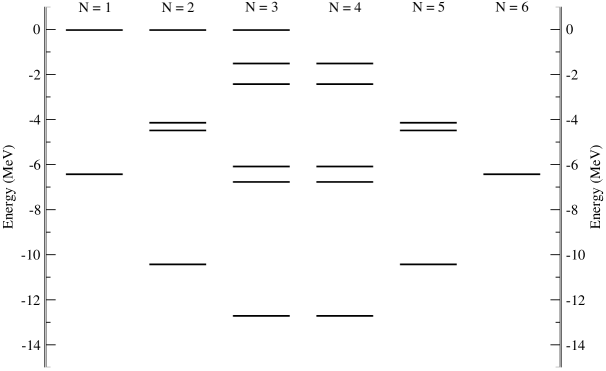
Figure 1: Energy eigenvalues for $N=1-6$ pairs of nucleons in the first nuclear $sd$ shell. The coefficients $c_{j}$ and the pairing strength $|G|$ are those from Pan:1997rw . Note the spectral symmetry discussed in the text and also the absence of the zero energy states for the nuclei corresponding to more than half full shell.

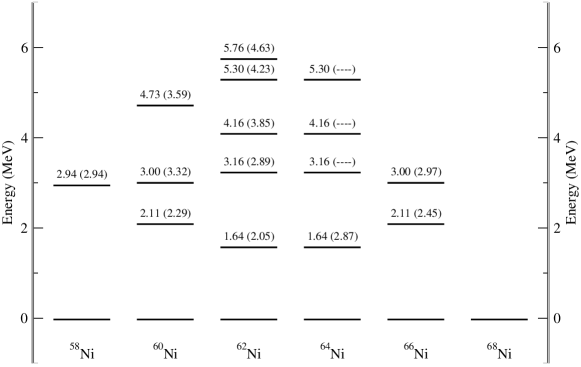
Figure 2: Excitation spectra for Ni isotopes and comparison with experimental results (in brackets) auerbach .

Energy/$-|G|$	State
$0$	$\displaystyle\frac{c_{j_{2}}c_{j_{3}}}{\Omega_{j_{1}}}d_{23}\left(a_{123}+\Gamma\right)S_{1}^{+}|0\rangle+\frac{c_{j_{1}}c_{j_{3}}}{\Omega_{j_{2}}}d_{31}\left(a_{231}+\Gamma\right)S_{2}^{+}|0\rangle+\frac{c_{j_{1}}c_{j_{2}}}{\Omega_{j_{3}}}d_{12}\left(a_{312}+\Gamma\right)S_{3}^{+}|0\rangle$
	$\displaystyle\frac{c_{j_{2}}c_{j_{3}}}{\Omega_{j_{1}}}d_{23}\left(a_{123}-\Gamma\right)S_{1}^{+}|0\rangle+\frac{c_{j_{1}}c_{j_{3}}}{\Omega_{j_{2}}}d_{31}\left(a_{231}-\Gamma\right)S_{2}^{+}|0\rangle+\frac{c_{j_{1}}c_{j_{2}}}{\Omega_{j_{3}}}d_{12}\left(a_{312}-\Gamma\right)S_{3}^{+}|0\rangle$
$\displaystyle\Omega_{j_{1}}|c_{j_{1}}|^{2}+\Omega_{j_{2}}|c_{j_{2}}|^{2}+\Omega_{j_{3}}|c_{j_{3}}|^{2}$	$\displaystyle c^{*}_{j_{1}}\hat{S}^{+}_{j_{1}}|0\rangle+c^{*}_{j_{2}}\hat{S}^{+}_{j_{2}}|0\rangle+c^{*}_{j_{3}}\hat{S}^{+}_{j_{3}}|0\rangle$

Table 5: Energies and eigenstates for three levels and one pair of nucleons. Here, $d_{kl}$, $a_{klm}$ and $\Gamma$ are defined in Eqs. (59), (60) and (61), respectively.

In order to test our formalism, we produce the excitation spectra for six Ni isotopes, ^58-68Ni (see Fig. 2), corresponding to nuclei with one to six pairs of neutrons that occupy the first nuclear $pf$ shell above the ⁵⁶Ni vacuum. We use the occupation numbers from auerbach and fit the pairing strength $G$ to reproduce the experimental first excited $0^{+}$ state of ⁵⁸Ni. The results are in very good agreement with experiment table .

V Conclusions and Outlook

In this paper, we showed that the Bethe ansatz technique can be applied to the nuclear pairing Hamiltonian with separable pairing strengths and degenerate single particle energy levels in a purely algebraic fashion. This algebraic method reveals a symmetry between the energy eigenstates corresponding to at most half full shell and those corresponding to more than half full shell. Namely, the eigenstates with $N$ pairs of nucleons where $N\leq N_{max}/2$ and the eigenstates with $N_{max}+1-N$ pairs of nucleons have the same energy and these states can be found by solving the same equations of Bethe ansatz. This symmetry is shadowed by the effects which are not considered in this paper but nevertheless it is manifest for the pure pairing Hamiltonian. Using this symmetry, we are now able to complete the pairing spectra obtained by Pan et al Pan:1997rw for the first nuclear $sd$ shell. We have also shown that the zero energy states do not obey this symmetry because they do not exist for more than half full shell.

Once the pairing spectra is obtained by solving the relevant equations of Bethe ansatz, one way to account for the effects of the nondegeneracy of single particle energy levels is to consider the one body term as perturbation. If the separations between the single particle energy levels within the shell are small compared to the pairing strength $|G|$, then one obtains small corrections to the pairing spectra. These corrections separate the degenerate zero energy states and shift the other states.

The Bethe ansatz technique presented here is especially powerful if the last shell of the isotope in consideration is almost empty or almost full. Because in this case one can find the eigenstates and the energies by solving only a few BAE’s as seen in Table 1. Even if the number of levels in the shell is large, these equations contain only a few variables and therefore can be solved conveniently.

We also would like to point out that, in the formalism developed here, one can use different occupation probabilities for different isotopes. Although we construct the Bethe ansatz states starting from the empty (or fully occupied) shell and one by one creating (or destroying) nucleon pairs, the pairing Hamiltonian is actually number conserving. As a result, the eigenstates presented in Table 1 with different number of pairs can be treated as eigenstates of different Hamiltonians with different occupation probabilities.

In this paper, we also considered a shell with two levels in detail. Although the two level system is of less physical interest, it helps us to present an alternative method of solving the equations of Bethe ansatz. This method has certain advantages over the conventional brute force approach. We showed that, in this special case, the problem of solving the equations of Bethe ansatz for zero energy eigenstates can be transformed into the problem of finding the roots of a certain hypergeometric polynomial. Here, the order of the polynomial is equal to the number of pairs in consideration. This allows us to find analytical solutions for up to $4$ pairs of nucleons. For higher number of pairs, one can find the roots numerically using well established algorithms. Even in this case, finding the roots of the hypergeometric polynomial numerically is considerably easier than solving the corresponding equations of Bethe ansatz which are coupled and nonlinear. Roots of various hypergeometric polynomials and their properties are studied by many groups (see for example Zeros and the references therein). We would like to add that although the technique presented here works only for a shell with two levels, it nevertheless hints to a potentially beneficial way of approaching the Bethe ansatz equations, in general. The extensions of the technique to shells with higher number of levels or to the BAE’s for nonzero energy states remain to be studied.

Appendix A The Bethe Ansatz Formalism

In this Appendix, we briefly outline the details of the calculations leading to the results of Section II.B. Let us start with a Bethe ansatz state of the form

$$\hat{S}^{+}(y_{1})\hat{S}^{+}(y_{2})\dots\hat{S}^{+}(y_{N})|0\rangle.$$ (62)

This state has $N$ nucleon pairs and we assume that $2\leq N\leq N_{max}/2$. We also assume that the variables $y_{k}$ are all different from each other. Using form of the Hamiltonian given in Eq. (10), together with Eqs. (13) and (22)-(24), it is straightforward show that the action of the pairing Hamiltonian on the state in Eq. (62) is

$$\hat{H}\hat{S}^{+}(y_{1})\hat{S}^{+}(y_{2})\dots\hat{S}^{+}(y_{N})|0\rangle$$

$$= -2|G|\left(K(y_{1})+\sum_{k\neq 1}^{N}\frac{1}{y_{1}-y_{k}}\right)\hat{S}^{+}(0)\hat{S}^{+}(y_{2})\hat{S}^{+}(y_{3})\dots\hat{S}^{+}(y_{N})|0\rangle$$

$$- 2|G|\left(K(y_{2})+\sum_{k\neq 2}^{N}\frac{1}{y_{2}-y_{k}}\right)\hat{S}^{+}(y_{1})\hat{S}^{+}(0)\hat{S}^{+}(y_{3})\dots\hat{S}^{+}(y_{N})|0\rangle$$

$$- \dots$$

$$- 2|G|\left(K(y_{N})+\sum_{k\neq N}^{N}\frac{1}{y_{N}-y_{k}}\right)\hat{S}^{+}(y_{1})\hat{S}^{+}(y_{2})\hat{S}^{+}(y_{3})\dots\hat{S}^{+}(0)|0\rangle.$$

Here, $K(x)$ is given by

$$K(y)=\sum_{j}\frac{\Omega_{j}/2}{1/|c_{j}|^{2}-y}.$$ (64)

Clearly, if we set $y_{k}=x^{(N)}_{k}$, where $x^{(N)}_{k}$ are the solutions of the BAE’s (38), then all the terms on the right hand side of Eq. (A) vanish. This proves that the state given by Eq. (37) is an eigenstate of the pairing Hamiltonian with zero energy.

Alternatively, we can set $y_{1}=0$ and $y_{k}=z^{(N)}_{k-1}$ for $k=2,3,\dots,N$ where $z^{(N)}_{m}$ are solutions of Eqs. (30). Then, using Eqs. (30) and (64), we can show that all the terms in Eq. (A) vanish except the first one. In other words, (A) reduces to

$$\hat{H}\hat{S}^{+}(0)\hat{S}^{+}(z^{(N)}_{1})\dots\hat{S}^{+}(z^{(N)}_{N-1})|0\rangle=-2|G|\left(K(0)-\sum_{k=1}^{N-1}\frac{1}{z^{(N)}_{k}}\right)\hat{S}^{+}(0)\hat{S}^{+}(z^{(N)}_{1})\dots\hat{S}^{+}(z^{(N)}_{N-1})|0\rangle.$$ (65)

This shows us that the state (29) is an eigenstate. Using Eqs. (64) and (65), one can easily show the energy of this state is given by Eq. (32).

Let us now consider a Bethe ansatz state in the following form:

$$\hat{S}^{-}(y_{1})\hat{S}^{-}(y_{2})\dots\hat{S}^{-}(y_{N-1})|\bar{0}\rangle.$$ (66)

Here, $|\bar{0}\rangle$ is the state representing the full shell defined in Eq. (14). The operators $\hat{S}^{-}(y)$ annihilate $N-1$ nucleon pairs so that the state in Eq. (66) has $N_{max}+1-N$ nucleon pairs. Since we assume that $N\leq N_{max}/2$, this state corresponds to a shell which is more than half full. Using the form of the Hamiltonian given in Eq. (10), together with Eqs. (15)-(16) and (22)-(24), it can be shown that the action of the pairing Hamiltonian on the state (66) is

$$\hat{H}\hat{S}^{-}(y_{1})\hat{S}^{-}(y_{2})\dots\hat{S}^{-}(y_{N-1})|\bar{0}\rangle$$

$$= 2|G|\left(-K(0)+\sum_{k=1}^{N-1}\frac{1}{y_{k}}\right)\hat{S}^{-}(y_{1})\hat{S}^{-}(y_{2})\dots\hat{S}^{-}(y_{N-1})|\bar{0}\rangle$$

$$- 2|G|\left(K(y_{1})+\frac{1}{y_{1}}+\sum_{k\neq 1}^{N-1}\frac{1}{y_{1}-y_{k}}\right)\hat{S}^{-}(0)\hat{S}^{-}(y_{2})\dots\hat{S}^{-}(y_{N-1})|\bar{0}\rangle$$

$$- 2|G|\left(K(y_{2})+\frac{1}{y_{2}}+\sum_{k\neq 2}^{N-1}\frac{1}{y_{2}-y_{k}}\right)\hat{S}^{-}(y_{1})\hat{S}^{-}(0)\dots\hat{S}^{-}(y_{N-1})|\bar{0}\rangle$$

$$- \dots$$

$$- 2|G|\left(K(y_{N-1})+\frac{1}{y_{N-1}}+\sum_{k\neq N-1}^{N-1}\frac{1}{y_{N-1}-y_{k}}\right)\hat{S}^{-}(y_{1})\hat{S}^{-}(y_{2})\dots\hat{S}^{-}(0)|\bar{0}\rangle.$$

Here, $K(y)$ is given by Eq. (64). If we set $y_{k}=z^{(N)}_{k}$, where $z^{(N)}_{k}$ are the solutions of the BAE’s (30), then the state (66) becomes the state in Eq. (31). In this case, using Eqs. (30) and (64), we can show that Eq. (A) reduces to

$$\hat{H}\hat{S}^{-}(z_{1}^{(N)})\hat{S}^{-}(z_{2}^{(N)})\dots\hat{S}^{-}(z_{N-1}^{(N)})|\bar{0}\rangle=2|G|\left(-K(0)+\sum_{k=1}^{N-1}\frac{1}{z^{(N)}_{k}}\right)\hat{S}^{-}(z_{1}^{(N)})\hat{S}^{-}(z_{2}^{(N)})\dots\hat{S}^{-}(z_{N-1}^{(N)})|\bar{0}\rangle.$$ (68)

This tells us that the state (31) is also an eigenstate of the pairing Hamiltonian. Its energy can be shown to be as in Eq. (32), using Eqs. (68) and (64).

References

• (1) R.W. Richardson, Phys. Rev. 159, 792 (1967).
• (2) A.K. Kerman, Ann. Phys. (NY) 12, 300 (1961); A.K. Kerman, R.D. Lawson, and M.H. MacFarlane, Phys. Rev. 124, 162 (1961)
• (3) I. Talmi, Nucl. Phys. A172, 1 (1971).
• (4) F. Pan, J. P. Draayer and W. E. Ormand, Phys. Lett. B 422, 1 (1998) [arXiv:nucl-th/9709036].
• (5) A. Volya, B. A. Brown and V. Zelevinsky, Phys. Lett. B 509, 37 (2001) [arXiv:nucl-th/0011079].
• (6) R.W. Richardson, Phys. Lett. B 3, 277 (1963); M. Gaudin, J. Physique 37, 1087 (1976); M. Gaudin, La Fonction d’onde de Bethe, Collection du Commissariat a l’énergie atomique, Masson, Paris, 1983.
• (7) A. B. Balantekin, T. Dereli and Y. Pehlivan, J. Phys. G 30, 1225 (2004) [arXiv:nucl-th/0407006].
• (8) T.J. Stieltjes, 1914 Sur Quelques Theoremess d’Algebre, Oeuvres Completes, V. 11 (Groningen:Noordhoff).
• (9) Higher Transcendental Functions, Volume 1, Ed. A. Erdelyi, McGraw-Hill, 1953.
• (10) N. Auerbach, Nucl. Phys. 76, 321 (1966).
• (11) Table of Isotopes, Volume 1, Ed. V. S. Shirley, John Wiley & Sons, 1996.
• (12) K. Boggs and P.Duren, Computational Methods and Function Theory 1 (2001), 275-287.