the CJT calculation in studying nuclear matter beyond mean field approximation

Abstract

We have introduced a CJT calculation in studying nuclear matter beyond mean field approximation. Based on the CJT formalism and using Walecka model, we have derived a set of coupled Dyson equations of nucleons and mesons. Neglecting the medium effects of the mesons, the usual MFT results could be reproduced. The beyond MFT calculations have been performed by thermodynamic consistently determining the meson effective masses and solving the coupled gap equations for nucleons and mesons. The numerical results for the nucleon and meson effective masses at finite temperature and chemical potential in nuclear matter are discussed.

I Introduction

Mean field theory (MFT) has an important role in the study of nuclear matter. Based on quantum hadrodynamics (QHD) and by mean field approximation, one can obtain the results in good agreement with the properties of the nuclear matter, like saturation density and binding energy, etc ref1 ; ref2 ; ref3 . For Walecka model (QHD-I), mean field approximation could be regarded as replacing the meson fields by their expectation value ref4 . That is to say treating the meson fields as the classical fields while quantum fluctuation ignored. From a Green’s function formalism, the mean field approximation could also be viewed as resumming all the tad-pole graphs in the nucleon self-energy ref5 ; ref6 . If one wants to make calculations beyond MFT, one should systematically calculate the higher loop contributions from a self-consistent resummation scheme. At the same time it is important to preserve the thermodynamic consistency ref6a . By the one particle irreducible effective action formalism, when evaluated to two loops, the calculations become very involved and after taking certain approximations the results are found to be not consistent with the properties of the nuclear matter ref7 . In principle the higher loop contributions should give reasonable results. Therefore one should find systematic and consistent resummation scheme and make proper approximations to obtain soundable results beyond mean field calculation.

For the effective action formalism, the effective action $\Gamma(\phi)$, which is the generating functional of one particle irreducible graphs, could been systematically calculated by summing all the relevant Feynman graphs to a given order of the loop expansion ref8 ; ref9 ; ref10 ; ref11 . However in this scheme it is not convenient to preserve the consistency of the effective action and the full propagators at the same order of the approximation. A generalized effective action for composite operators has been developed by Cornwall, Jackiw and Tomboulis (CJT) ref12 . According to CJT formalism the usually effective action $\Gamma(\phi)$ is generalized to depend not only on $\phi(x)$, a possible expectation value of the quantum field $\Phi(x)$, but also on $G(x,y)$, a possible expectation value of the time-ordered product $T\Phi(x)\Phi(y)$. $G(x,y)$ is also the full propagator of the field. In this case the effective action $\Gamma(\phi,G)$ is the generating functional of the two particle irreducible graphs. An effective potential $V(\phi,G)$ can be defined by removing an overall factor of space-time volume of the effective action. Physical solutions demand minimization of the effective potential with respect to both $\phi$ and $G$ ref12 , which means

$$\frac{\partial V(\phi,G)}{\partial\phi}=0$$ (1)

and

$$\frac{\partial V(\phi,G)}{\partial G}=0.$$ (2)

This formalism was originally written at zero temperature. Then it had been extended at finite temperature by Amelino-Camelia and Pi where it was used for investigations of the effective potential of the $\lambda\phi^{4}$ theory ref13 and gauge theories ref14 . In the study of the spontaneous symmetry breaking system, $\phi$ is also the order parameter of the transition and nonzero; while in the system without spontaneous symmetry breaking, this parameter is zero. For the thermodynamic system the effective potential could be identified as the thermodynamic potential. One can use the CJT formalism to study nuclear matter. In our previous work ref15 , we have already applied the CJT formalism to the study of nuclear matter. At the first step, after the proper approximations we have successfully reproduced the MFT results through the CJT formalism. And we have also illustrated that the thermodynamic consistency is preserved in the CJT formalism. In this paper we will further study how to make thermodynamic consistent calculations beyond MFT in the CJT formalism.

The organization of the present paper is as follows: In section 2, we formulate the CJT formalism in the study of nuclear matter by the Walecka model. The thermodynamic potential and coupled Dyson equations of the full propagators are derived at Hartree-Fock approximation. In section 3, we will make the beyond MFT calculations by including the medium effects of the mesons in a thermodynamic consistent way and give our numerical results. The last section comprises a summary and discussion.

II CJT formalism in nuclear matter

We start from the QHD-I Lagrangian which can be written as

$${\cal L}=\bar{\psi}(i\gamma_{\mu}\partial^{\mu}-m_{N}+g_{\sigma}\sigma-g_{\omega}\gamma_{\mu}\omega^{\mu})\psi+\frac{1}{2}(\partial_{\mu}\sigma\partial^{\mu}\sigma-m_{\sigma}^{2}\sigma^{2})-\frac{1}{4}F_{\mu\nu}F^{\mu\nu}+\frac{1}{2}m_{\omega}^{2}\omega_{\mu}\omega^{\mu},$$ (3)

where $\psi$, $\sigma$ and $\omega$ are the fields of the nucleon, sigma meson and omega meson respectively and $F_{\mu\nu}=\partial_{\mu}\omega_{\nu}-\partial_{\nu}\omega_{\mu}$. According to the Lagrangian we can write down the free propagators of the nucleon, sigma meson and omega meson respectively as

$$G_{0}(p)=\frac{i}{/\!\!\!p-m_{N}},$$ (4)

$$\Delta_{0}(p)=\frac{i}{p^{2}-m_{\sigma}^{2}},$$ (5)

$$D_{0}^{\mu\nu}(p)=\frac{-ig^{\mu\nu}}{p^{2}-m_{\omega}^{2}}.$$ (6)

We will use the imaginary-time formalism to compute quantities at finite temperature ref16 . Our notation is

$$\int_{p}f(p)\equiv\frac{i}{\beta}\sum_{n}\int\frac{d^{3}\bf p}{(2\pi)^{3}}f(p_{0}=i\omega_{n},{\bf p}),$$ (7)

where $\beta$ is the inverse temperature, $\beta=1/T$. We have $\omega_{n}=2n\pi T$ for boson and $\omega_{n}=(2n+1)\pi T$ for fermion, where $n=0,\pm 1,\pm 2,\cdots$. A baryon chemical potential $\mu$ can be introduced by replacing $p_{0}=i\omega_{n}$ with $p_{0}=i\omega_{n}+\mu$ in the nucleon propagator.

According to the CJT formalism ref12 , the expansion of the effective potential or the thermodynamic potential of the nuclear matter can be written as

$$\Omega(G,\Delta,D)=i\int_{p}Tr\ln G_{0}(p)G^{-1}(p) + i\int_{p}Tr\left[G_{0}^{-1}(p)G(p)-1\right]-\frac{i}{2}\int_{p}\ln\Delta_{0}(p)\Delta^{-1}(p)-\frac{i}{2}\int_{p}\left[\Delta_{0}^{-1}(p)\Delta(p)-1\right]$$ (8)

$$- \frac{i}{2}\int_{p}\ln D_{0}(p)D^{-1}(p)-\frac{i}{2}\int_{p}\left[D_{0}^{-1}(p)D(p)-1\right]+\Omega_{2}(G,\Delta,D),$$

where $G$, $\Delta$ and $D$ are the full propagators of nucleon, $\sigma$ meson and $\omega$ meson respectively, which are determined by the stationary condition (2). $\Omega_{2}(G,\Delta,D)$ is given by all the two-particle irreducible vacuum graphs with all the propagators treated as the full propagators. In the CJT formalism at Hartree-Fock approximation $\Omega_{2}(G,\Delta,D)$ can be illustrated by the graphs of figure 1, where the solid lines repent $G(p)$, the dashed line represents $\Delta(p)$ and the wavy line represents $D^{\mu\nu}(p)$. The vertices for $\sigma\psi\bar{\psi}$ and $\omega^{\mu}\psi\bar{\psi}$ are $-g_{\sigma}$ and $g_{\omega}\gamma^{\mu}$ respectively.

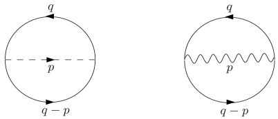
Figure 1: Hartree-Fock approximation to $\Omega_{2}(G,\Delta,D)$. The solid, dash and wavy lines are the nucleon propagator G, the $\sigma$ meson propagator $\Delta$ and the $\omega$ meson propagator $D$ respectively. $q$ and $p$ are the four momenta.

The analytic expression is

$$\Omega_{2}(G,\Delta,D)=\frac{ig_{\sigma}^{2}}{2}\int_{p}\int_{q}Tr\left[G(q)G(q-p)\Delta(p)\right]+\frac{ig_{\omega}^{2}}{2}\int_{p}\int_{q}Tr\left[\gamma^{\mu}G(q)\gamma^{\nu}G(q-p)D_{\mu\nu}(p)\right].$$ (9)

From the stationary condition (2) which demands that $\Omega(G,\Delta,D)$ be stationary against variations of $G$, $\Delta$ and $D$ respectively, we will have the following Dyson equations

$$G(q)^{-1} = G_{0}(q)^{-1}+g_{\sigma}^{2}\int_{p}G(q-p)\Delta(p)+g_{\omega}^{2}\int_{p}\gamma^{\mu}G(q-p)\gamma^{\nu}D_{\mu\nu}(p),$$ (10)

$$\Delta(p)^{-1} = \Delta_{0}(p)^{-1}-g_{\sigma}^{2}\int_{q}Tr\left[G(q)G(q-p)\right],$$ (11)

$$D_{\mu\nu}(p)^{-1} = D_{0,\mu\nu}(p)^{-1}-g_{\omega}^{2}\int_{q}Tr\left[\gamma_{\mu}G(q)\gamma_{\nu}G(q-p)\right].$$ (12)

The above equations can be also represented pictorially in figure 2.

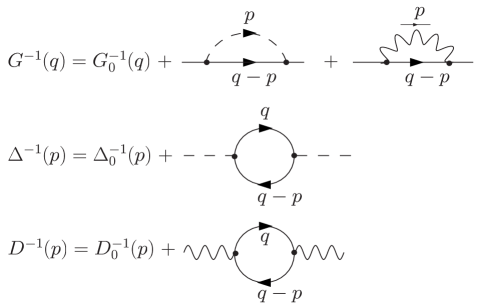
Figure 2: The Dyson equations satisfied by the nucleon, the $\sigma$ meson and the $\omega$ meson propagators at Hartree-Fock approximation. $q$ and $p$ are the four momenta.

These integration equations are nonlinear coupled and momentum dependent. Needless to say they are very difficult for computation. The certain approximations should be adopted.

III the beyond mean field CJT calculation and numerical results

In our previous study ref15 , in order to reproduce the mean field results through the CJT formalism, we have neglected the medium effects of the mesons which means the meson full propagators are replaced by their bare ones. The Dyson equations are decoupled and can be numerically solved. Then we could reproduce the correct saturation properties of nuclear matter as shown in figure 3. The coupling constants thus are fixed at $g_{\sigma}^{2}=155.6$ and $g_{\omega}^{2}=521.5$. The result from MFT is also presented for comparison in figure 3.

Figure 3: The average energy per nucleon minus the nucleon mass $m_{N}$ as functions of baryon density at zero temperature in the CJT formalism (solid line) and MFT (dashed line).

In this paper, we are going to make calculations beyond mean field. We will take the following ansatz of the meson full propagators

$$\Delta(p)=\frac{i}{p^{2}-M_{\sigma}^{2}},$$ (13)

$$D^{\mu\nu}(p)=\frac{-ig^{\mu\nu}}{p^{2}-M_{\omega}^{2}},$$ (14)

where $M_{\sigma}$ and $M_{\omega}$ are the effective masses of the $\sigma$ and $\omega$ mesons, which in principle should be determined by equation (11) and (12). However, as we have mentioned that the momentum dependent coupled Dyson equations are very difficult to be solved. So we have to find other simplified ways to determine the effective masses and meanwhile preserve the thermodynamic consistency.

The full nucleon propagator is taken as the following form

$$G(q)=\frac{i}{\gamma_{\mu}q^{\mu}-m_{N}+\Sigma},$$ (15)

where $\Sigma$ is the proper nucleon self-energy which will be determined by the equation (10). It can be generally written as

$$\Sigma(q)=\Sigma_{s}(q)-\gamma^{0}\Sigma_{0}(q)+{\bm{\gamma}}{\bm{\cdot}}{\bf q}\Sigma_{v}(q).$$ (16)

Thus we can define an effective nucleon mass

$$M_{N}(q)=m_{N}-\Sigma_{s}(q),$$ (17)

which is momentum dependent. As the nuclear matter is a uniform system at rest, the contribution of $\Sigma_{v}$ term in equation (16) is very small and usually neglected ref5 . So only $\Sigma_{s}$ and $\Sigma_{0}$ need to be evaluated.

By the above ansatz of the full propagators, the thermodynamic potential could be written as

$$\Omega(G,\Delta,D)= i \int_{p}Tr\ln G_{0}(p)G^{-1}(p)-\int_{p}Tr\left[G(p)\Sigma(p)\right]-\frac{i}{2}\int_{p}\ln\Delta_{0}(p)\Delta^{-1}(p)-\frac{1}{2}\int_{p}\left(M_{\sigma}^{2}-m_{\sigma}^{2}\right)\Delta(p)$$ (18)

$$- \frac{i}{2}\int_{p}\ln D_{0}(p)D^{-1}(p)+\frac{1}{2}\int_{p}\left(M_{\omega}^{2}-m_{\omega}^{2}\right)g_{\mu\nu}D^{\mu\nu}(p)+\Omega_{2}(G,\Delta,D).$$

From equation (10), (15) and (16), we could derive that

$$\Sigma(q)=ig_{\sigma}^{2}\int_{p}G(q-p)\Delta(p)+ig_{\omega}^{2}\int_{p}\gamma_{\mu}G(q-p)\gamma_{\nu}D^{\mu\nu}(p),$$ (19)

thus we have

$$\Omega_{2}(G,\Delta,D) = \frac{1}{2}Tr\int_{q}G(q)\left\{ig_{\sigma}^{2}\int_{p}G(q-p)\Delta(p)+ig_{\omega}^{2}\int_{p}\gamma_{\mu}G(q-p)\gamma_{\nu}D^{\mu\nu}(p)\right\}$$ (20)

$$= \frac{1}{2}\int_{q}Tr\left[G(q)\Sigma(q)\right].$$

In the next we will mainly calculate $\Sigma$, $M_{\sigma}$, $M_{\omega}$ and $\Omega$ in a thermodynamic consistency way. In the following calculations the vacuum fluctuations will be neglected. The $\Sigma(q)$ could be evaluated from equation (19). The momentum dependence can be eliminated if we define the nucleon effective mass as the pole mass of the full propagator ref16a in the limit ${\bf q}\to 0$ as discussed in ref15 . With the $\Sigma_{v}$ term dropped we have

$$\Sigma = \Sigma_{s}-\gamma^{0}\Sigma_{0},$$ (21)

$$\Sigma_{s} = -g_{\sigma}^{2}\int\frac{d^{3}\bf p}{(2\pi)^{3}}\frac{M_{N}}{2E_{\sigma}E}\frac{2(M_{N}-E)n_{\sigma}-E_{\sigma}(\tilde{n}_{+}+\tilde{n}_{-})}{(M_{N}-E)^{2}-E_{\sigma}^{2}}+g_{\omega}^{2}\int\frac{d^{3}\bf p}{(2\pi)^{3}}\frac{2M_{N}}{E_{\omega}E}\frac{2(M_{N}-E)n_{\omega}-E_{\omega}(\tilde{n}_{+}+\tilde{n}_{-})}{(M_{N}-E)^{2}-E_{\omega}^{2}},$$ (22)

$$\Sigma_{0} = g_{\sigma}^{2}\int\frac{d^{3}\bf p}{(2\pi)^{3}}\frac{-(\tilde{n}_{+}-\tilde{n}_{-})}{2(M_{N}-E)^{2}-2E_{\sigma}^{2}}+g_{\omega}^{2}\int\frac{d^{3}\bf p}{(2\pi)^{3}}\frac{-(\tilde{n}_{+}-\tilde{n}_{-})}{(M_{N}-E)^{2}-E_{\omega}^{2}},$$ (23)

where $E_{\sigma/\omega}=\sqrt{{\bf p^{2}}+m_{\sigma/\omega}^{2}}$ and $E=\sqrt{{\bf p}^{2}+M_{N}^{2}}$; the Bose and Fermion distribution functions are

$$n_{\sigma/\omega}=\frac{1}{e^{\beta E_{\sigma/\omega}}-1},\ \ \ \ \ \ \tilde{n}_{\pm}=\frac{1}{e^{\beta(E\mp\mu^{*})}+1},$$ (24)

where $\mu^{*}=\mu-\Sigma_{0}$ and $\mu$ is the baryon chemical potential.

After performing the frequency sums in equation (18) and neglecting the vacuum fluctuations, the thermodynamic potential could be evaluated as

$$\Omega(\mu,T)= - 4T\int\frac{d^{3}\bf p}{(2\pi)^{3}}\left[\ln(1+e^{-\beta(E-\mu^{*})})+\ln(1+e^{-\beta(E+\mu^{*})})\right]$$ (25)

$$+ 4M_{N}\Sigma_{s}\int\frac{d^{3}\bf p}{(2\pi)^{3}}\frac{1}{E}(\tilde{n}_{+}+\tilde{n}_{-})-4\Sigma_{0}\int\frac{d^{3}\bf p}{(2\pi)^{3}}(\tilde{n}_{+}-\tilde{n}_{-})$$

$$+ T\int\frac{d^{3}\bf p}{(2\pi)^{3}}\ln(1-e^{-\beta E_{\sigma}})-\frac{1}{2}(M_{\sigma}^{2}-m_{\sigma}^{2})\int\frac{d^{3}\bf p}{(2\pi)^{3}}\frac{n_{\sigma}}{E_{\sigma}}$$

$$+ 4T\int\frac{d^{3}\bf p}{(2\pi)^{3}}\ln(1-e^{-\beta E_{\omega}})-2(M_{\omega}^{2}-m_{\omega}^{2})\int\frac{d^{3}\bf p}{(2\pi)^{3}}\frac{n_{\omega}}{E_{\omega}}+\Omega_{2},$$

where

$$\Omega_{2}=-2M_{N}\Sigma_{s}\int\frac{d^{3}\bf p}{(2\pi)^{3}}\frac{1}{E}(\tilde{n}_{+}+\tilde{n}_{-})+2\Sigma_{0}\int\frac{d^{3}\bf p}{(2\pi)^{3}}(\tilde{n}_{+}-\tilde{n}_{-}).$$ (26)

The $\Sigma_{s}$ and $\Sigma_{0}$ in $\Omega_{2}$ will be evaluated in the forms of equations (22) and (23). Now we are in a position to determine the effective masses $M_{\sigma}$ and $M_{\omega}$. In equation (25), $M_{\sigma}$ and $M_{\omega}$ could be viewed as independent variables. As known that a thermodynamic system in equilibrium will minimize its thermodynamic potential to these independent variables, which means

$$\frac{\partial\Omega}{\partial M_{\sigma}}=0,\ \ \ \ \ \frac{\partial\Omega}{\partial M_{\omega}}=0.$$ (27)

$M_{\sigma}$ and $M_{\omega}$ determined in this way are momentum independent and the thermodynamic consistency is certainly preserved. From equation (25), the two equations in (27) could be written as

$$\frac{1}{2}(M_{\sigma}^{2}-m_{\sigma}^{2})\frac{\partial}{\partial M_{\sigma}}\int\frac{d^{3}{\bm{p}}}{(2\pi)^{3}}\frac{n_{\sigma}}{E_{\sigma}}+2M_{N}\int\frac{d^{3}{\bm{p}}}{(2\pi)^{3}}\frac{1}{E}(\tilde{n}_{+}+\tilde{n}_{-})\frac{\partial\Sigma_{s}}{\partial M_{\sigma}}-2\int\frac{d^{3}{\bm{p}}}{(2\pi)^{3}}(\tilde{n}_{+}-\tilde{n}_{-})\frac{\partial\Sigma_{0}}{\partial M_{\sigma}}=0,$$ (28)

$$(M_{\omega}^{2}-m_{\omega}^{2})\frac{\partial}{\partial M_{\omega}}\int\frac{d^{3}{\bm{p}}}{(2\pi)^{3}}\frac{n_{\omega}}{E_{\omega}}+M_{N}\int\frac{d^{3}{\bm{p}}}{(2\pi)^{3}}\frac{1}{E}(\tilde{n}_{+}+\tilde{n}_{-})\frac{\partial\Sigma_{s}}{\partial M_{\omega}}-\int\frac{d^{3}{\bm{p}}}{(2\pi)^{3}}(\tilde{n}_{+}-\tilde{n}_{-})\frac{\partial\Sigma_{0}}{\partial M_{\omega}}=0.$$ (29)

The equations (22), (23), (28) and (29) form a set of closed equations from which $\Sigma_{s}$, $\Sigma_{0}$, $M_{\sigma}$ and $M_{\omega}$ could be numerically solved. At this stage we could make calculations and discussions beyond MFT in studying nuclear matter. As an application we will discuss the temperature and chemical potential dependence of the effective masses of nucleons, $\sigma$ mesons and $\omega$ mesons in the hot and dense nuclear matter.

Figure 4: The effective nucleon masses as functions of temperature at zero chemical potential in the CJT formalism (solid line) and MFT (dashed line).

At zero chemical potential, we could discuss the temperature dependence of the effective masses. In figure 4 the nucleon effective mass of the CJT case decreases with temperature increasing. At low temperature the effective mass decreases very slowly. At certain high temperature the effective mass becomes decreasing fast with temperature increasing. The MFT result is also plotted for comparison. We could see that when temperature is high the effective mass decreases more rapidly in the CJT case than that of the MFT case. In figure 5 the meson effective masses as functions of temperature are plotted. The effective mass of $\sigma$ meson increases with temperature increasing. At high temperature it increases more obviously. While The effective mass of $\omega$ meson will decrease with temperature increasing. It decreases more quickly at high temperature.

Figure 5: The effective masses of $\sigma$ and $\omega$ mesons as functions of temperature at zero chemical potential in the CJT formalism.

At given temperature, we could also study the chemical potential dependence of the effective masses. In figure 6 we could see that the nucleon effective masses decrease with chemical potential increasing at different given temperatures. From low temperature to high temperature the effective masses decrease more and more remarkably with chemical potential increasing. In the CJT case the effective masses decrease more rapidly with chemical potential than that in the MFT case at high temperatures.

Figure 6: The effective nucleon masses as functions of chemical potential at different given temperatures in the CJT formalism (solid line) and MFT (dashed line).

We show in figures 7 and 8 the $\sigma$ and $\omega$ effective masses as functions of chemical potential at different give temperatures. The $\sigma$ effective masses increase with the increase of the chemical potential while the $\omega$ effective masses decrease with the increase of the chemical potential at given temperature. For both $\sigma$ and $\omega$ mesons, the effective masses change slightly with chemical potential at low given temperatures but rapidly at high given temperatures.

Figure 7: The $\sigma$ effective masses as functions of chemical potential at different given temperatures in the CJT formalism .

Figure 8: The $\omega$ effective masses as functions of chemical potential at different given temperatures in the CJT formalism .

IV summary

By the CJT formalism and Walecka model, we have made a beyond MFT calculation in studying nuclear matter. We derive a coupled Dyson equations for the full propagators of nucleons and mesons. After neglecting the vacuum fluctuations and the momentum dependence in the nucleon self-energies, the nucleon self-energies can be evaluated by the Dyson equation of the nucleon full propagator, while the meson effective masses are determined by minimizing the thermodynamic potential to these effective masses instead of directly evaluating the meson Dyson equations. This kind of treatment simplifies the calculation meanwhile preserves the thermodynamic consistency. The effective masses and thermodynamic potential can be numerical evaluated at given chemical potential and temperature. The numerical results show that the nucleon effective mass decreases with the increase of temperature or chemical potential, and it decreases more rapidly in the CJT case than that of the MFT case. For the mesons, the effective mass of $\omega$ meson decreases with temperature or chemical potential increasing, while the effective mass of $\sigma$ meson increases with temperature or chemical potential increasing. Both nucleon and meson effective masses change more quickly at high temperature or chemical potential than that at low temperature or chemical potential.

References

• (1) R.J. Furnstahl, B.D. Serot, Comments Nucl.Part.Phys. 2 (2000) A23.
• (2) B.D. Serot, J.D. Walecka, Int.J.Mod.Phys. E6 (1997) 515.
• (3) B.D. Serot, Rep.Prog.Phys. 55 (1992) 1855.
• (4) J.D. Walecka, Theoretical Nuclear and Subnuclear Physics, Oxford Univ. Press, 1995.
• (5) B.D. Serot, J.D. Walecka, Adv.Nucl.Phys. 16 (1986) 1.
• (6) S.A. Chin, Ann.Phys. 108 (1977) 301.
• (7) H. Uechi, Phys. Rev. C41 (1990) 744.
• (8) R.J. Furnstahl, R.J. Perry, B.D. Serot, Phys.Rev. C40 (1989) 321.
• (9) R. Jackiw, Phys.Rev. D9 (1974) 1689.
• (10) L. Dolan, R. Jackiw, Phys.Rev. D9 (1974) 3320.
• (11) S. Coleman, E. Weinberg, Phys.Rev. D7 (1973) 1888.
• (12) A. Linde, Rep.Prog.Phys. 42 (1979) 390.
• (13) J. Cornwall, R. Jackiw, E. Tomboulis, Phys.Rev. D10 (1974) 2428.
• (14) G. Amelino-Camelia, So-Young Pi, Phys.Rev. D47 (1993) 2356.
• (15) G. Amelino-Camelia, Phys.Rev. D49 (1994) 2740.
• (16) Song Shu, Jia-Rong Li, Nucl.Phys. A760 (2005) 369.
• (17) J. Kapusta, Finite-Temperature Field Theory, Cambridge Univ. Press, 1989.
• (18) S. Gao, Y.-J. Zhang, R.-K. S, Phys.Rev. C52 (1995) 380.