Influence of Meson’s Widths on
Yukawa-like Potentials and Lattice Correlation Functions

Abstract

Euclidean point-to-point propagators or wall-to-wall correlators related to exchange by an unstable particle ($\sigma,\rho,\omega$-mesons) are modified by presence of particle width. In particular, the usual method of deriving particle masses from logarithmic derivatives need to be modified. Similarly Yukawa-like potentials of nuclear physics due to exchange of those mesons are significantly modified since the coupling to the decay products is strong. For example, the large distance asymptotic changes, $\sim\exp(-M_{min}r)$, where $M_{min}$ is the sum of the decay product masses ($2m_{\pi},2m_{e},2m_{\nu}$). In the area $M_{min}r<1$ the potential has a long-range tail $\sim 1/r^{3}$. Similar effects appear due to the virtual decays in the elecroweak sector of the Standard model. The $Z-\gamma$ mixing via electron loop gives the parity violation potential with the range $1/2m_{e}$, i.e. the range of the weak interaction increases $10^{5}$ times.

I Introduction

This paper addresses the following general question: what is the role, if any, of a width $\Gamma$ of an unstable particle in situations in which this particle is a $virtual$ intermediate state so that its physical decay $cannot$ take place. We will discuss three applications of such kind:
(i) Euclidean $point-to-point$ correlation functions in which particles in question are emitted and absorbed by two operators acting at 4-d points;
(ii) Euclidean $wall-to-wall$ correlators, widely used on the lattice for determination of particle masses; in this case a signal is emitted and absorbed from 3-d planes separated by some time interval $\tau$;
(iii) Yukawa-like potentials due to meson exchanges widely used in nuclear physics, this case can be called $line-to-line$ correlators.

The cases (ii) and (iii) are schematically illustrated in Fig.1: although those have direct applications, the corresponding results simply follow from those of the generic case (i), the point-to-point Euclidean propagator. There are of course other similar situations in which the same ideas apply but not discussed below: t-channel meson exchange in scattering amplitudes is another example. There would be no difficulty to generalize what is done below to these case as well. Also let us add that although we call unstable particle a meson, it can equally well be any other unstable particle with non-negligible width (e.g. the $Z$ boson of weak interaction).

Figure 1: The setting for (a) wall-to-wall and (b) line-to-like Euclidean correlators, describing Euclidean lattice correlators and exchange potentials, respectively. The unstable article propagation is indicated by a dashed line.

To set up a problem, let us first explain why naive Euclidean continuation of the real-time amplitudes does $not$ work. Usual real-time amplitudes describing resonances behave as damped oscillators

$$A(t)\sim exp(-iMt-\Gamma t/2)$$ (1)

Their naive Euclidean rotation, by simple substitution $t\rightarrow-i\tau$ which leads to an oscillating function $\sim exp(-M\tau+i\Gamma\tau/2)$ which certainly cannot be true Euclidean propagators or amplitudes. In fact those are defined via real exponent of the Hamiltonian $\sim exp(-\hat{H}\tau)$ and standard spectral decomposition plus Hermitian Hamiltonian of course demands all energy to be real and thus the correlator to decrease monotonously with $\tau$.

Why should one seek an answer to such questions? Apart of being the basis of applications of statistical mechanics, Euclidean correlation functions with real exponentials of $\hat{H}$ are the main tool of lattice gauge theory community, which studies the non-perturbative dynamics of non-Abelian gauge fields by numerical simulations, see multiple reviews e.g. lat_revew . Rotation to Euclidean time is also a crucial ingredient of the semiclassical approach based on instantons, see e.g.reviewinst_rev . These correlators are widely used to extract the particle masses and their couplings to certain currents, but it was not yet used to extract the widths of resonances. We will see below that it is indeed not a simple task.

The present-day lattice calculations have practical limitations stemming from available computer resources. As a result, quark used are still rather heavy, so that in most calculations the pions are so heavy that no decays of $\sigma$ and $\rho$ are possible. Another kinematical effects is a consequence of small size of the present-day lattices $L\sim 2$ fm. Indeed, momentum quantization of the decay products due to the periodic boundary conditions to $p_{n}=2\pi n/L$ also prevents decay in many cases, especially with the the initial “plane-to-plane” projection to $\vec{p}=0$.

This paper is not addressing these lattice limitations, considering ideal case with quark masses at its physical value and $L$ large enough to cause no problem. The issue we address is how a propagator of unstable particle look like, when it is virtual and is propagating either in space direction (related to Yukawa potentials below) or in imaginary (Euclidean) time. As we will see, the widths can modify the shape of these propagators , sometimes beyond recognition. Although masses and widths can still be extracted from those correlators, it would require very complicated fitting procedure. For the same reason, using lattice simulations for the evaluation of the transport properties via Kubo-like formulae from Euclidean correlators is practically impossible, as discussed e.g. in PetTeaney .

Our approach is based on standard dispersion relations, which connect real part of the amplitudes in momentum representation to their imaginary part, also known as spectral densities, in which resonances appear as Breit-Wigner-like peaks. If the resonance width is very small, those can be approximated by delta functions and the width ignored. If so, the usual exponential behavior of the wall-to-wall Euclidean correlators $K(\tau)\sim exp(-M\tau)$ or standard Yukawa-like potentials $V(r)\sim exp(-Mr)/r$ are obtained. If the width is small, one can perform a saddle point integration and find analytically the first corrections to delta function, in form of some “shifted mass” depending on the width $\Gamma$. If the width is not small, the form of the correlators or potentials is strongly modified, as it will be detailed below.

Another related issue is modification of hadronic resonances at finite temperatures. We will not discuss here multiple physical effects which are important in resonance emission from “heat baths” created e.g. in heavy ion collisions, but just comment on the simplest “kinematical” effect BrownShu which appear even in high energy elementary $pp$ collisions. When the spectral density is convoluted with the thermal Boltzmann exponent, the finite width of a resonance leads to different weighting of the left and right side of the peak and thus an apparent resonance mass shift. For small width and/or high temperature it is very easy to estimate the effect: approximating the resonance as

$${exp(-M/T)\over 1+(4/\Gamma^{2})(M-m_{res})^{2}}\approx$$ (2)

$$exp[-({4\over\Gamma^{2}})(M^{2}-2Mm_{res}-M^{2}+{2M\Gamma^{2}\over 8T}]$$

one gets the mass shift to be

$$\delta m_{max}\approx m_{0}-{\Gamma^{2}\over 8T}$$ (3)

This simple analytic expression however does not work well in practice and real shift depends much on the resonance shape (see BrownShu for details).

II Point-to-point correlators, dispersion relations and the spectral density

We start with the point-to-point correlation functions because other cases can easily be obtained from them, by integration. In fact point-to-point correlators in Euclidean space-time are not just methodical object, they are important tools widely used in studies of structure of the QCD vacuum. They can be deduced phenomenologically, using vast set of data accumulated in hadronic physics. Second, they can be directly calculated ab initio using quantum field theory methods, such as lattice gauge theory, or semiclassical methods. Significant amount of work has also been done in order to understand their small-distance behavior, based on the Operator Product Expansion, see SVZ_79 and vast subsequent literature.

These correlation functions are vacuum expectation value of the product of two (or more) of operators

$$K(x-y)=<0|O(x)O(y)|0>$$ (4)

which can have any gauge invariant combination of fields, for example mesonic operators we will consider have local quark-antiquark combination

$$O_{mes}(x)=\bar{\psi}_{i}M_{ij}\psi_{j}$$ (5)

where a matrix M can include various flavor and Dirac structures, and a convolution over quark color indices. Since the vacuum is homogeneous, the correlators depend on the relative distance only. If two points are inside the light cone, a lot of things may happen: e.g. a meson may decay in between. We will not consider such case below, always assuming that the distance between the points (x-y) is space-like. It may really be a space distance or “Euclidean time” interval: in both cases there are no real decays and one deals with monotonously decreasing functions of the distance.

The Fourier transform of $K(x)$, $K_{mom}(q^{2})$, depends on the momentum transfer $q$ flowing from one operator to another. In its language, the situation we consider corresponds only to virtual space-like 4-momenta $q$ $Q^{2}=-q^{2}>0$, like in scattering experiments in which the resonance is in $t$ and not $s$ channels.

Due to causality, standard dispersion relations follow: they relate real and imaginary parts

$$K_{mom}(q^{2})=\int{ds\over\pi}{ImK_{mom}(s)\over(s-q^{2})}$$ (6)

where the r.h.s. is the physical spectral density $ImK_{mom}(s)$. It certainly is non-zero only for positive $s$ above certain threshold (twice the pion mass in the case of $\rho,\sigma$ resonances to be considered.

Dispersion relation is the basis of various sum rules. Their general idea is as follows; suppose one knows the l.h.s. $K_{mom}(q^{2})$ somewhere; thus some integral in the r.h.s. of the physical spectral density is known as well. (For example, for mesonic operators the correlators at small x are just given by free quark propagation $K\sim 1/x^{6}$, with calculable corrections.) The simplest of them use directly momentum space: those are known as finite energy sum rules. Unfortunately, those are not very useful because most of the dispersion integrals are divergent and to usable sum rules appear only after some “subtractions”, which introduces extra parameters and undermine their prediction power.

Improved sum rules appear if one takes a sufficient number of derivatives of the dispersion relation at $Q=0$, defining the so called moments of the spectral density

$$M_{n}=\int{ds\over\pi}{ImK_{mom}(s)\over s^{n+1}}$$ (7)

Following Shifman,Vainshtein and Zakharov SVZ_79 , this method is traditionally used in the discussion of “charmonium sum rules” related to correlators of $\bar{c}c$ currents. Another idea also suggested by these authors SVZ_79 is to introduce the so called Borel transform of the function $K_{mom}(Q)$ defined as follows

$$K_{bor}(m)=lim_{n,Q^{2}\rightarrow\infty,m^{2}=Q^{2}/n^{2}=fixed}$$

$${Q^{2n}\over(n-1)!}(-{d\over dQ^{2}})^{n}K_{mom}(Q^{2})$$ (8)

leading to “Borel-transformed” sum rules

$$K_{bor}(m)=\int{ds\over\pi}ImK_{mom}(s)exp(-{s\over m^{2}})$$ (9)

in which the integral is cut off at large $s$ exponentially. Such form of the sum rules have been widely used in multiple papers based on the QCD sum rules.

Another natural option, advocated by one of us in Shu_cor , is to use the sum rules directly in the (Euclidean) coordinate representation. By applying Fourier transformation to (6) one obtains the following nearly self-explanatory form

$$K(x)=\int{ds\over\pi}ImK_{mom}(s)D(s^{1/2},x)$$ (10)

The former function in the r.h.s. describes the amplitude of production of all intermediate states of mass $\sqrt{s}$, while the latter

$$D(m,x)=(m/4\pi^{2}x)K_{1}(mx)$$ (11)

is nothing else but the Euclidean propagator of a mass-$s$ state to the distance $x$. At large $x$ the propagator goes as $exp(-mx)$, thus it is also exponentially cut off and, in practice, there is little difference between this expression and Borel sum rules . However the coordinate form can be much easier evaluated numerically, on the lattice or in semiclassical models, unlike the Borel-transformed version. As discussed in Shu_cor and subsequent literature, for vector and axial correlators one can directly use experimental data and calculate the l.h.s. with rather small error bars. This can provide a very good test of lattice calculations. The inverse transformation – from correlators to spectral densities – is a badly defined problem, quite difficult in practice, except in some simplest situations.

Now, let us think about a situation in which the lowest state in the corresponding channel is an $unstable$ particle – for example $\rho,\omega$ mesons for vector operators or $\sigma$ for scalar isoscalar operator $\bar{q}q$. In the simplest case of very narrow resonance in which the width of the resonance is neglected, one simply gets the propagator of a state with the resonance mass $M$ $K(x)\sim D(M,x)$. If the width is small, one can use the same idea as for the thermal case, leading to analog of the formula (3) with the temperature $T$ replaced by $1/x$. If the width is substantial, the integral in (10) should be calculated more accurately, with the appropriate shape of the resonance. We will show how this procedure works in the next section.

III Wall-to-wall correlators and lattice measurements of hadronic masses

Although there is quite substantial literature on lattice point-to-point correlators, most of studies rely on wall-to-wall correlation functions, obtained from K(x) by additional integration over the 3-dimensional spacial plane. This puts the momentum of all intermediate states to be zero, so dispersion relation in this case can be considered to be related not to the mass of the state but simply to its energy. The resulting function is related to the physical spectral density by

$$K_{wall-to-wall}(\tau)=\int{dm\over\pi}ImK_{mom}(m)exp(-\tau m)$$ (12)

where 4-d propagator $D$ is substituted by its 1-d version.

The mass of the lowest hadrons is traditionally obtained from the logarithmic derivative of such correlators

$$E(\tau)=-\frac{dlogK}{d\tau}\rightarrow_{\tau\rightarrow\infty}M$$ (13)

Indeed, multiple lattice calculations have been able to show that the logarithmic derivative of wall-to-wall correlators do have “plateaus” independent of $\tau$, being the standard source of the meson masses.

Such procedure works well in present-day calculations in which kinematical effects mentioned above prevent decays. However, as the algorithms and supercomputers gets more powerful, the widths eventually would become an issue.

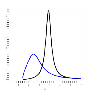
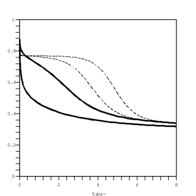
Figure 2: (a) The shape of $\rho$ (right) and $\sigma$ resonance, as a function of its mass m ($fm^{-1}$). (b) The corresponding logarithmic derivative of the wall-to-wall correlator $E(\tau)\,(GeV)$ vs Euclidean time $\tau(fm)$. The solid curves are for $\rho$ (higher) and $\sigma$ resonances (both mass and width are 450, MeV), two dashed curves are for $\rho$ with the width reduced to $\Gamma_{0}=15,1.5\,MeV$, (lower and upper, respectively).

Let us demonstrate what should happen with “mass plateaus” by calculating them for different resonance shape. The simplest case in which an analytic formula is easily obtained is a Gaussian resonance $\sim exp[-4*(m-m0)^{2}/\Gamma^{2}]$ for which the mass integral can be taken from minus to plus infinity and

$$E(\tau)=m-\tau\Gamma^{2}/8$$ (14)

But this dependence does not reproduce what happens for realistic shapes of the resonances, with a particular dependence of the width on energy, especially near the threshold. The best way is to calculate numerically the behavior of $E(\tau)$ for realistic spectral densities, and see what should its true shape for vector and scalar currents be. The most studied vector currents have two lowest resonances, I=1 $\rho$ meson and I=0 $\omega$. In principle, the spectral densities describe continuum of states, all the way from the lowest physical states (2 and 3 pions at rest) respectively. So, one may only argue that the logarithmic derivatives is limited by $2m_{\pi}$ or $3m_{\pi}$ from below.

A reasonably good parameterization of the spectral density $ImK_{mom}$ for binary channels is Breit-Wigner

$$\rho(M)={\Gamma(M)\over(M-m_{res})^{2}+\Gamma(M)^{2}/4}$$ (15)

where the width is not constant and depends on the current running mass $M$ and angular momentum of the resulting pions. Due to P-wave nature of $\rho\rightarrow\pi\pi$ decay, its $\Gamma_{\rho}(M)=\Gamma_{\rho}^{0}(1-4m_{\pi}^{2}/M^{2})^{3/2}$, while for $s$-wave $\sigma$ resonance one should use the power $1/2$ instead. The corresponding shape of the resonances is shown in Fig.2(a): we do not show here fitting of the real data, although we have checked that these shapes do indeed agree with them.

The resulting “realistic” logarithmic derivative of the meson contribution is shown in Fig.2(b). Let us start its discussion with two dashed curves, which are for $\rho$ meson with the width artificially reduced by the factor 100 (upper dashed) and 10 (lower dashed curve) compared to real-world $\Gamma_{0}=.14\,GeV$. These two curves nicely show “plateaus” at the rho mass $M_{\rho}=.77\,GeV$ at not-too-large $\tau$, with a “slide” toward the threshold ($2m_{\pi}$) at large $\tau$. However for the realistic width value (the solid curve) the rho meson mass plateau is already gone, with a slide of $E(\tau)$ even at small $\tau$. The situation is even more dramatic for the sigma meson, for which the mass-to-width ratio is 1:1. Presumably by fitting such curves, if they come from correlator studues, one would still be able to recover both the mass and the meson width, but we leave this for further studies.

It may be useful to have some analytical estimates for $K(\tau)$. Let us start from large $\tau$. In this case small $m$ dominate in the integral (12) and we can substitute $m=2m_{\pi}(1+x)$ assuming $x<<1$. The result is

$$K(\tau)=const\frac{2m_{\pi}\Gamma_{0}}{(m_{res}-2m_{\pi})^{2}}\frac{exp(-2m_{\pi}\tau)}{(m_{\pi}\tau)^{q+1}},$$ (16)

$$E(\tau)=-\frac{dlogK}{d\tau}=2m_{\pi}+(q+1)/\tau,$$ (17)

where $q=3/2$ for $\rho$ and $q=1/2$ for $\sigma$. This should be compared to the resonance contribution $K^{r}(\tau)=exp(-m_{r}\tau)$. Only if this term dominates, we have $E^{r}(\tau)\approx m_{r}$. However, for $\rho$ and $\sigma$ the coefficient $2m_{\pi}\Gamma_{0}/(m_{res}-2m_{\pi})^{2}$ is not small, therefore, the asymptotic regime starts very early. The transitional area corresponds to $2m_{\pi}<1/\tau<m_{r}$. Here an essential contribution comes from the integration interval $2m_{\pi}<m<m_{r}$: $K^{tr}(\tau)\sim\Gamma_{0}/(\pi(m_{res}-2m_{\pi})^{2}\tau)$. If this contribution dominates we have $E^{tr}(\tau)\approx 1/\tau$. Note that the value of the width actually determines the position of the transition point between the areas of the resonance and non-resonance domination in $K(\tau)$ or $E(\tau)$. Therefore, both the meson mass and width can, in principle, be found from the fit of lattice calculations.

IV Yukawa-like potential due to exchange by an unstable particle

Let us consider the potential between two nucleons produced by a meson (e.g. $\sigma,\rho,\omega$) exchange. For brevity we omit all isotopic and kinematic structures which are different for different particles and may be easily restored in the final answers. This potential in the coordinate representation may be presented as an integral of its imaginary part in the momentum representation

$$U(r)=\frac{1}{4\pi^{2}r}\int^{\infty}_{2m}{\rm Im}U(M)\exp(-rM)2MdM\ ,$$ (18)

One can either consider this expression as simply a line-to-line variant of the Euclidean correlators, with 3-d Green function $exp(-Mr)/r$ substituting 4-d one in (10), or follow the usual derivation of the Uehling potential in textbooks (such as berestetskii ). The lower limit of the integration is determined by the minimal mass $2m$ of the decay products ($\pi$-mesons) of the intermediate particle and

$${\rm Im}U(M)=-{\rm Im}\frac{4\pi g_{1}g_{2}}{M^{2}-M_{0}^{2}-P(M)}=$$ (19)

$$\frac{4\pi g_{1}g_{2}m_{r}\Gamma(M)}{(M^{2}-M_{m}^{2})^{2}+m_{r}^{2}\Gamma^{2}(M)}\ .$$ (20)

Here $g_{1},g_{2}$ are the meson-nucleon interaction constants, $P(M)$ is the polarization operator,$M_{0}$ is the bare meson mass, $M_{m}=M_{m}(M)=\sqrt{M_{0}^{2}+{\rm Re}P(M)}$ is the running meson mass, $m_{r}=M_{m}(m_{r})=\sqrt{M_{0}^{2}+{\rm Re}P(m_{r})}$ is the meson mass at the resonance, and ${\rm Im}P(M)\equiv-m_{r}\Gamma(M)$ where $\Gamma(M)$ is the running meson width.

Substituting Eq. (19) into Eq.(18) we obtain

$$U(r)=\frac{g_{1}g_{2}m_{r}}{\pi r}\int^{\infty}_{2m}\frac{\Gamma(M)\exp(-rM)}{(M^{2}-M_{m}^{2})^{2}+m_{r}^{2}\Gamma^{2}(M)}dM^{2}.$$ (21)

The explanation of this formula, like other Euclidean correlators above, is simple: the mass $M$ of the unstable particle is not fixed and therefore the potential can be seen as an the integral over all possible meson masses given by the spectral density (e.g. a modified Breit-Wigner formula we use).

In the case of vanishingly small $\Gamma(M)$ the Breit-Wigner factor in Eq. (21) is proportional to $\delta$-function and the integration gives the usual Yukawa potential:

$$U(r)=\frac{g_{1}g_{2}}{r}\exp(-rm_{r})$$ (22)

Non-zero width $\Gamma(M)$ produces significant deviations from the simple Yukawa formula. The potential $U(r)$ in Eq. (21) can be easily found using numerical integration. At Fig.3 we presented graphs of two ratios: $\rho$-meson potential divided by the Yukawa potential and $\sigma$-meson potential divided by the Yukawa potential . We see that the deviations from the Yukawa formula may be very large, especially at large distances. Below we perform analytical estimates to explain the nature of different corrections to Yukawa formula. For the analytical estimates we assume $m<<m_{r}$ and $\Gamma_{r}<<m_{r}$ where $\Gamma_{r}=\Gamma(m_{r})$ is the resonance width.

Figure 3: The ratios of $\rho$-meson potential to Yukawa potential (thick solid line) and $\sigma$-meson potential to Yukawa potential (dashed line) as functions of $m_{r}r$. At $m_{r}r<4$ the negative corrections given in Eq.(30) dominate. At $m_{r}r>4$ the positive corrections Eqs.(24-26) change the long-range behavior of the potentials.

The integral has four important intervals of the integration: the first interval is near the threshold, $M\sim 2m$; the second interval is $2m<<M<<m_{r}$; the third interval is near the resonance, $M\sim m_{r}$; and the fourth interval is $\Gamma_{r}<<M-m_{r}<infinity$. Therefore, the potential may be presented as a sum of four terms

$$U(r)=U_{2m}(r)+U_{p}(r)+U_{res}(r)+U_{inf}(r)$$ (23)

Consider first a behavior of the potential (21) at large distance, $rm_{r}>>1$. In this case the threshold interval $M\sim 2m$ gives the dominating contribution. The width $\Gamma(M)$ vanishes near the threshold as $\Gamma(M)=(1-4m^{2}/M^{2})^{q}\cdot\Gamma_{0}$ where $q=1/2$ for $\sigma$-meson (the $\pi$-mesons are in $s$-wave; for $Z$-boson $q=1/2$ too) and $q=3/2$ for $\rho$- meson (the $\pi$-mesons are in $p$-wave). Taking $M=2m(1+x)<<m_{r}$ we obtain

$$U_{2m}(r)=\frac{D_{q}g_{1}g_{2}\exp(-2mr)}{r(mr)^{q+1}}$$ (24)

$$D_{q}=\frac{2^{3/2-q}(2q)!!m_{r}m^{2}\Gamma_{0}}{(M_{m}^{2}(2m)-4m^{2})^{2}}\sim\frac{m^{2}\Gamma_{0}}{m_{r}(m_{r}-2m)^{2}}$$ (25)

In the estimate we assumed $M_{m}(2m)\approx m_{r}$. This contribution has the same nature as the Uehling potential produced by virtual “decay” of photon to electron-positron pair ($q=1/2$).

Consider now the interval of the integration $2m<<M<<m_{r}$ which corresponds to the distances $1/m_{r}<<r<<1/m$. The result of the integration in this area is

$$U_{p}(r)=\frac{2g_{1}g_{2}\Gamma(r^{-1})}{\pi m_{r}^{3}r^{3}}$$ (26)

The potentials $U_{p}\propto 1/r^{3}$ ($1/m_{r}<<r<<1/m$) and $U_{2m}\propto\exp(-2mr)/r^{q+2}$ ($r>>1/m$) cover the area $r>>1/m_{r}$. The potential here is exponentially enhanced in comparison with the Yukawa potential- see Fig.3. In the region $r\sim 1/m_{r}$ the resonance contribution dominates. To estimate the correction to the Yukawa potential we present the integral in Eq. (21) in the following form:

$$U_{res}(r)=\frac{g_{1}g_{2}m_{r}\exp(-rm_{r})}{\pi r}I(r)$$ (27)

$$I(r)=\int^{\infty}_{2m}\frac{\exp[r(m_{r}-M)]\Gamma_{r}2MdM}{[(M^{2}-m_{r}^{2})^{2}+m_{r}^{2}\Gamma_{r}^{2}]}$$ (28)

$$\approx\int^{\infty}_{0}\frac{[1-r(M-m_{r})]\Gamma_{r}2MdM}{[(M^{2}-m_{r}^{2})^{2}+m_{r}^{2}\Gamma_{r}^{2}]}.$$ (29)

This gives an estimate of the corrections to the Yukawa potential

$$U_{res}(r)\approx\frac{g_{1}g_{2}}{r}\exp(-rm_{r})(1-\Gamma_{r}r/\pi-\Gamma_{r}/(\pi m_{r})).$$ (30)

Thus, to use Yukawa potential we must assume $\Gamma_{r}<<\pi m_{r}$ and $\Gamma_{r}r<<\pi$. Then we should add $U_{p}$ or $U_{2m}$ in the area $m_{r}r>1$.

The behaviour of the potential at small distances depends on the convergence of the integral in the area $m<<M<1/r$. For mesons of finite size the integral is convergent at $r=0$ and $U_{inf}(r)$ should be neglected. The meson exchange theory of strong interaction is not applicable at small distance anyway.

Now we can compare our analytical estimates with numerical calculations presented at Fig.3. To calculate the integral in Eq.(21) we take
$\Gamma(M)=[(1-4m^{2}/M^{2})/(1-4m^{2}/m_{r}^{2})]^{q}\cdot\Gamma_{r}$;
$\Gamma_{r}/m_{r}=0.19$, $2m/m_{r}=0.36$ and $q=3/2$ for $\rho$-meson; $\Gamma_{r}/m_{r}=1$, $2m/m_{r}=0.5$ and $q=1/2$ for $\sigma$-meson. The condition $\Gamma_{r}<<m_{r}$ is not satisfied for $\sigma$-meson. Nevertheless, the negative corrections $1-\Gamma_{r}r/\pi-\Gamma_{r}/(\pi m_{r})$ given in Eq.(30) correctly explain behavior of both potentials at $m_{r}r<1$ (including the negative slope for $m_{r}r<0.5$, see Fig.4 ). For $m_{r}r<3$ the $\rho$-meson potential in Eq.(21) is about 10% smaller than the Yukawa potenatial, the $\sigma$-meson potential is about 40% smaller. At $m_{r}r>5$ the positive corrections Eqs.(24-26) give dominating contribution and change the long-range behavior of the potentials.

Finally, let us consider potential $U(r)$ in the short-range approximation,

$$U(r)\approx B\frac{4\pi g_{1}g_{2}}{m_{r}^{2}}\delta(r),$$ (31)

$$B=\frac{m_{r}^{2}}{4\pi g_{1}g_{2}}\int U(r)d^{3}r=$$ (32)

$$\frac{2}{\pi}\int^{\infty}_{2m/m_{r}}\frac{\gamma(x)dx}{x[(x^{2}-1)^{2}+\gamma^{2}(x)]},$$ (33)

where $x=M/m_{r}$ and $\gamma(x)=\Gamma(M)/m_{r}$. This short-range approximation may also be useful in the calculation of the nuclear mean field. The numerical integration gives $B=0.93$ for $\rho$-meson and $B=0.62$ for $\sigma$-meson.

It may also be useful to have some analytical estimates for $B$. In the logarithmic approximation

$$B\approx[1+\frac{\Gamma_{0}}{\pi m_{r}}(\ln{\frac{m^{2}_{r}}{4m^{2}}}-const)].$$ (34)

It is interesting that the logarithmic correction diverges at $m=0$. This happens because of the long-range character of the potential in the area $1/m_{r}<<r<<1/m$. Indeed, the integration of $U_{p}(r)\propto 1/r^{3}$ from Eq.(26) immediately gives this logarithmic correction to $B$ . However, for real mesons $\ln[(m_{r}/(2m)]\sim 1$ and the negative correction factor $1-\Gamma_{r}/(\pi m_{r})$ to the resonance contribution ( see Eq.(30)) is more important. In fact, numerical results for $B$ are surprisingly close to this correction. Indeed, $1-\Gamma_{r}/(\pi m_{r})=0.94$ and $B=0.93$ for $\rho$-meson; $1-\Gamma_{r}/(\pi m_{r})=0.68$ and $B=0.62$ for $\sigma$-meson. This gives a very simple rough estimate for the effect of large width for the mesons: multiply the Yukawa potential by the factor $1-\Gamma_{r}/(\pi m_{r})$. The results of this prescription in comparison with real potentials are shown at Fig.4.

Figure 4: The ratios of $\rho$-meson potential to Yukawa potential (thick solid line) and $\sigma$-meson potential to Yukawa potential (thick dashed line) as functions of $m_{r}r$. Thin dashed lines show factors $1-\Gamma_{r}/(\pi m_{r})$.

V Long-range parity violating potential

The $Z$-boson exchange creates a parity violating potential. A possibility of a longer range of such potential could have interesting applications, for example, in atomic tests of the Standard Model (see e.g. review of atomic parity violation in ginges and a different mechanism for a long-range parity violating potential in F ). Note that the case of $Z$-boson differs from the meson case. The imaginary part of the polarization operator for point-like particles like photon and $Z$-boson rapidly increases with $M$. For example, the electron contribution to the photon vacuum polarization is berestetskii

$${\rm Im}P(M)=-\frac{\alpha}{3}(1-\frac{4m^{2}}{M^{2}})^{1/2}(2m^{2}+M^{2})$$ (35)

For the $Z$-boson we need to sum over all decay channels, however, it does not change the conclusions. First consequence of ${\rm Im}P(M)\propto M^{2}$ is that the high-energy contribution to the integral (21) gives famous running coupling constants (correction $U_{inf}(r)\propto\ln{mr}/r$). The second consequence is the strong dependence of the running width $\Gamma(r^{-1})$ on $r^{-1}$ in Eq. (26) since in this case $\Gamma(r^{-1})\sim\alpha(m^{2}+r^{-2})/m_{r}$. Therefore, the dominating contribution in the area $1/m_{r}<<r<<1/m$ is actually $U_{p}(r)\propto 1/M_{Z}^{4}r^{5}$. As a result, the correction to the short-range approximation, $U(r)=\frac{4\pi g_{1}g_{2}}{m_{r}^{2}}\delta(r)$, remains finite for $m=0$ (for example, for zero neutrino mass). However, the $Z-\gamma$ mixing via electron loop gives a long-range contribution (the second term below) to the parity violating electron-nucleus interaction

$$W=\frac{G}{2\sqrt{2}}\gamma_{5}[-Q_{w}\rho(r)+Z\frac{2\alpha(1-4sin^{2}\theta_{w})m_{e}^{2}}{3\pi^{2}r}I(r)]$$ (36)

$$I(r)=\int^{\infty}_{1}\exp(-2xm_{e}r)\sqrt{x^{2}-1}(1+\frac{1}{2x^{2}})dx\,\,$$ (37)

Here the first term is the usual parity violating electron-nucleus interaction (see e.g. ginges ); $G$ is the Fermi constant, $\gamma_{5}$ is the Dirac matrix, $Q_{w}\approx-N+Z(1-4sin^{2}\theta_{w})$ is the weak charge, $Z$ and $N$ are numbers of protons and neutrons, $\theta_{w}$ is the Weinberg angle, $\rho(r)$ is the nuclear density normalised to 1 ($\rho(r)\approx\delta(r)$), $m_{e}$ is the electron mass. To obtain this potential we used the imaginary part of the polarization operator from Eq.(35) and the Standard model values of the interaction constants . The integral has the following asymptotics: for $m_{e}r\ll 1$

$$I(r)=\frac{1}{(2m_{e}r)^{2}}.$$ (38)

This gives $W\propto 1/r^{3}$. For $m_{e}r\gg 1$

$$I(r)=\frac{\sqrt{\pi}\exp(-2m_{e}r)}{4(m_{e}r)^{3/2}}.$$ (39)

This gives $W\propto\exp(-2m_{e}r)/r^{5/2}$. Thus, we have the parity violating potential with the range $1/(2m_{e})$. A similar effect appears for the nuclear-spin-dependent part of the parity violating interaction.

Acknowledgments.   This work was partially supported by the US-DOE grants DE-FG02-88ER40388 and DE-FG03-97ER4014, Australian Research Council and Gordon Godfrey fund.

References

- (1) M. Creutz, L. Jacobs and C. Rebbi, Phys. Rept. 95, 201 (1983).
- (2) T. Schafer and E. V. Shuryak, Rev. Mod. Phys. 70, 323 (1998) [arXiv:hep-ph/9610451].
- (3) E. V. Shuryak and G. E. Brown, Nucl. Phys. A 717, 322 (2003) [arXiv:hep-ph/0211119].
- (4) G. Aarts and J.M. Martinez Resco, JHEP 0204:053,2002, hep-ph/0203177. P. Petreczky and D. Teaney, Phys. Rev. D 73, 014508 (2006) [arXiv:hep-ph/0507318].
- (5) M. A. Shifman, A. I. Vainshtein and V. I. Zakharov, Nucl.Phys. B147, 385 (1979).
- (6) E. V. Shuryak, Rev. Mod. Phys. 65, 1 (1993).
- (7) V.B. Berestetskii, E.M. Lifshitz, and L.P. Pitaevskii, Relativistic Quantum Theory (Pergamon Press, Oxford, 1982).
- (8) M. Cristoforetti, P. Faccioli and M. Traini, arXiv:hep-ph/0701223.
- (9) J.S.M. Ginges, V.V. Flambaum. Phys. Rep. 397, 63 (2004) [arXiv:physics/0309054].
- (10) V.V.Flambaum. Phys. Rev. A 45, 6174 (1992).
- (11) N. Mathur et al., arXiv:hep-ph/0607110.