USTC-ICTS-06-05
Nucleon-antinucleon Interaction from the Modified Skyrme Model

Abstract

We calculate the static nucleon-antinucleon interaction potential from the modified Skyrme model with additional $B^{\mu}B_{\mu}$ term using the product ansatz. The static properties of single baryon are improved in the modified Skyrme model. State mixing is taken into account by perturbation theory, which substantially increases the strength of the central attraction. We obtain a long and mid range potential which is in qualitative agreement with some phenomenological potentials.

PACS numbers:13.75.Cs, 12.39.Dc, 11.10.Lm

I introduction

The Skyrme model is considered as the low energy limit of the quantum chromodynamics(QCD), it models QCD in the classical or large number of colors ($N_{C}$) limit and baryon is regarded as the soliton in the pion field skyrme1 ; skyrme2 ; adkins1 ; adkins2 . Upon quantizing a slowly rotating Skyrmion, static property of nucleons and $\Delta$ have been calculated with the results in agreement with experimental data within 30% adkins1 ; adkins2 . Recently it has been widely used to discuss the exotic hadrons exotic ; YLWM ; DY05 . The minimal version of the model consists of the following Lagrangian terms: the non-linear Sigma term with chiral order $\mathcal{O}(p^{2})$ and the Skyrme term with $\mathcal{O}(p^{4})$. Even though the minimal version of Skyrme model (Min-SKM) can be regarded as a successful phenomenological model in spite of its simplicity, it can not be used to study the problem of quark spin contents of proton or EMC effects yan ; yan1 ; Dia which are important QCD effects in baryon physics. This is a very unsatisfied defect for Min-SKM. In order to cure this disease, additional terms with $\mathcal{O}(p^{6})$ or high orders have to be added into the model’s Lagrangian to construct modified Skyrme Models. Among them, the simplest one is the model with the Min-SKM Lagrangian plus only one additional $B_{\mu}B^{\mu}$ term yan1 , where $B_{\mu}$ is the baryon current ( or Goldstone-Wilczek current ). Hereafter, we shortly call this simplest modified Skyrme model as Mod-SKM. It is expected that the Mod-SKM should be more realistic than Min-SKM. To discuss this issue, and to fix the parameters in Mod-SKM is one of the aims of this paper. Moreover the Mod-SKM can be obtained by considering the infinite $\omega$ mass limit of the vector meson $\omega$ term of the chiral Lagrangian studied in Ref adkins3 .

An interesting application of the Skyrme model is the investigation of the baryon-baryon interaction, especially the nucleon-nucleon($NN$) interaction nucleon1 ; nucleon2 ; nucleon3 ; nucleon4 ; nucleon5 ; nucleon6 . The Skyrme picture gives us a qualitative understanding of the principal features of the $NN$ interaction: it has the correct long-range one pion exchange potential which dominates the tensor force. There is a strong short range repulsion, and finally there is a pronounced central attraction at intermediate range, albeit weakly attractive while comparing with the phenomenological potential. However, the recent development of obtaining the $NN$ interaction from the Skyrme model has shown that the combined effect of the careful treatment of the nonlinear equations and the configuration mixing is to give substantial central midrange attraction for the $NN$ system that is in qualitative agreement with the data nucleon5 .

The $NN$ and $N\overline{N}$ potentials have been investigated by means of the Min-SKM and the algebraic methods in Ref. amado1 ; amado2 ; amado3 . The phenomenon and puzzles in the baryon-antibaryon physics have attracted much attention recently due to the remarkable discovery of baryon-antibaryon enhancements in the $J/\psi$ and $B$ decays Bes1 ; Bes2 ; Bes3 ; belle1 ; belle2 ; belle3 . The $N\overline{N}$ interaction and the possible nucleon-antinucleon bound states have been investigated from the constituent quark model constituent ; DY06 ; rDY06 . In the Skyrme model, the interactions between classical Skyrmion and antiskyrmion, i.e., $S\overline{S}$, were explored in YLWM ; DY05 . In the present paper, we shall study the $N\overline{N}$ potential using the Mod-SKM and following the methods developed in Refs. nucleon5 ; amado1 ; amado2 .

It is well-known that phenomenologically the $N\overline{N}$ potential is not as well established as the $NN$ potential. At distance less than about 1 fermi the interaction is dominated by annihilation. However, at larger distance, a meaningful potential can be defined and studied either by $G$ parity transformation on the $NN$ meson exchange potential or phenomenologically.

We will compare our Mod-SKM’s results to some phenomenological potentials. The $B^{\mu}B_{\mu}$ term in Mod-SKM reflects the effect of $\omega$ meson exchange adkins3 ; jackson ; oka . We will see that at large distance, where the product ansatz makes the best sense, the potentials based on the Skyrme model agree qualitatively and, in most cases, quantitatively with the phenomenological interactions. At intermediate and short distance, we do less well, but at these distances the product ansatz is not valid. However, the results are still suggestive.

In the following section, we give the Mod-SKM’s Lagrangian, then reproduce a number of static properties of single baryon which is both qualitatively appealing and quantitatively satisfactory. In Sec.III we study the skyrmion-antiskyrmion interaction in Mod-SKM, and project them to the nucleon space by the algebraic methods amado1 ; amado2 ; amado3 . We also consider the effects of rotational excitations by including intermediate states $\Delta$ and $\overline{\Delta}$, and evaluate the corrections to the $N\overline{N}$ potential in perturbation theory. Sec.IV closes this paper with some discussions related to the present study.

II the modified skyrme model and the static properties of single baryon

The Skyrme model lagrangian is generalized to include additional $B^{\mu}B_{\mu}$ term which simulates the effects of $\omega$ meson, and this modified Skyrme model lagrangian provides a better description of both the single baryon static properties and the low energy $NN$ interaction jackson ; oka . This lagrangian has the following form

$${\cal L}=\frac{F^{2}_{\pi}}{16}{\rm{Tr}}(\partial_{\mu}U\partial^{\mu}U^{{\dagger}})+\frac{1}{32e^{2}}{\rm{Tr}}([U^{\dagger}\partial_{\mu}U,U^{\dagger}\partial_{\nu}U]^{2})+\frac{1}{8}m^{2}_{\pi}F^{2}_{\pi}{\rm{Tr}}(U-1)-\frac{3\pi^{2}N_{C}}{5m^{2}}B^{\mu}B_{\mu}$$ (1)

where $U$ is a $SU(2)$ valued field $U=\exp[2i\tau_{a}\pi_{a}/F_{\pi}]$, $B^{\mu}$ is the topological current $B^{\mu}=\frac{1}{24\pi^{2}}\varepsilon^{\mu\nu\alpha\beta}{\rm{Tr}}[(U^{\dagger}\partial_{\nu}U)(U^{\dagger}\partial_{\alpha}U)(U^{\dagger}\partial_{\beta}U)]$, and $e,\;F_{\pi},\;m$ are parameters to be determined. The first term is the lagrangian of meson fields in the nonlinear sigma model and the second term is the so called Skyrme term which stabilizes the soliton. The third term is the pion mass term and the fourth term is the additional $B^{\mu}B_{\mu}$ term. $U$ transforms as $U\rightarrow U^{\prime}=LUR^{\dagger}$ under the chiral group $SU(2)_{L}\times SU(2)_{R}$, where both $L$ and $R$ are $SU(2)$ matrices.

The chiral soliton model adkins3 where, as an alternative to the Skyrme term, the vector meson $\omega$ term $\beta\omega^{\mu}B_{\mu}$ stabilizes the soliton, provides a support for the interpretation of the $B_{\mu}B^{\mu}$ term which emerges in the limit $m_{\omega}\rightarrow\infty$. In traditional nuclear interaction theories within the potential framework which are based on the single meson exchange mainly, it is shown that $N\overline{N}$ system is more attractive than the $NN$ system due to the fact that in the theories there is a strong $\omega$ exchange, so inclusion of this term which models the effect of the $\omega$ meson could help in a better description of the $N\bar{N}$ system. Furthermore, the study of the quark spin content also support that we should add this six derivative term in order to yield a spin content consistent with the present experiment yan ; spin . Generally terms in ${\cal L}$ with more than two time derivatives can lead to pathological runaway solutions when the adiabatic approximation is relaxed and present obvious difficulties in quantizing the theory. But the Lagrangian of Mod-SKM have, at most, two time derivatives, hence there is no such difficulty.

For the case with single static Skyrmion, we use the so called hedgehog ansatz:

$$U_{0}(\mathbf{r})=\exp[i\tau_{a}\hat{r}_{a}F(r)]$$ (2)

where $F(r)$ is the chiral angle which minimizes the static soliton energy subject to the boundary condition $F(0)=\pi$ and  $F(\infty)=0$. From Eq. (1)and Eq. (2), we get the mass of classical soliton:

$$M_{s}=\frac{\pi}{2}\frac{F_{\pi}}{e}\int_{0}^{\infty}\{x^{2}F^{\prime 2}+2S^{2}+4S^{2}(2F^{\prime 2}+\frac{S^{2}}{x^{2}})+2\mu^{2}x^{2}(1-C)+\nu^{2}\frac{S^{4}}{x^{2}}F^{\prime 2}\}$$ (3)

with

$$x=eF_{\pi}r,~{}~{}~{}\mu^{2}=\frac{m^{2}_{\pi}}{e^{2}F^{2}_{\pi}}\;,~{}~{}~{}F^{\prime}=\frac{dF}{dx}\;,$$

$$\nu^{2}=\frac{18e^{4}F^{2}_{\pi}}{5\pi^{2}m^{2}}\;,~{}~{}~{}S={\sin}F\;,~{}~{}~{}C={\cos}F.$$ (4)

In Eq. (3), the term proportional to $\nu^{2}$ comes from the $B^{\mu}B_{\mu}$ term and is absent in the conventional Skyrme model. Minimizing $M_{s}$ with respect to $F$, $\delta M_{s}=0$, we have the following equation for $F$,

$$(\frac{x^{2}}{4}+2S^{2}+\frac{\nu^{2}}{4}\frac{S^{4}}{x^{2}})F^{\prime\prime}+(\frac{\nu^{2}}{2}\frac{S^{3}C}{x^{2}}+2SC)F^{\prime 2}+(\frac{x}{2}-\frac{\nu^{2}}{2}\frac{S^{4}}{x^{3}})F^{\prime}-(\frac{1}{2}SC+\frac{2S^{3}C}{x^{2}}+\frac{1}{4}\mu^{2}x^{2}S)=0$$ (5)

From the above equation, we can see that the chiral angle $F$ asymptotically tends to the following expression when $r$ goes to infinity,

$$F(r)\rightarrow\mathcal{A}(\frac{1}{m_{\pi}eF_{\pi}r^{2}}+\frac{1}{eF_{\pi}r})\;e^{-m_{\pi}r}~{}~{}~{}(r\rightarrow\infty)$$ (6)

The coefficient $A$ is related to the pion-nucleon coupling constant $g_{{\pi}NN}$ through adkins1 ,

$$g_{{\pi}NN}=\frac{4{\pi}M_{N}\mathcal{A}}{3em_{\pi}}$$ (7)

Associated with the chiral symmetry, the vector current $J^{{\mu}a}_{V}$ and axial vector current $J^{{\mu}a}_{A}$ can be obtained from the Skyrme lagrangian Eq. (1) following the standard procedure,

$$J^{{\mu}a}_{V}=\frac{iF^{2}_{\pi}}{8}{\rm{Tr}}[\frac{\tau_{a}}{2}\;(\partial^{\mu}UU^{{\dagger}}+\partial^{\mu}U^{{\dagger}}U)]-\frac{i}{8e^{2}}{\rm{Tr}}\{[\frac{\tau_{a}}{2},\partial_{\nu}UU^{\dagger}][\partial^{\mu}UU^{\dagger},\partial^{\nu}UU^{\dagger}]$$

$$+[\frac{\tau_{a}}{2},\partial_{\nu}U^{\dagger}U][\partial^{\mu}U^{\dagger}U,\partial^{\nu}U^{\dagger}U]\}-\frac{3N_{C}i}{20m^{2}}\;\varepsilon^{\mu\nu\alpha\beta}B_{\nu}{\rm{Tr}}[\frac{\tau_{a}}{2}(\partial_{\alpha}UU^{{\dagger}}\partial_{\beta}UU^{{\dagger}}-\partial_{\alpha}U^{{\dagger}}U\partial_{\beta}U^{{\dagger}}U)],$$ (8)

$$J^{{\mu}a}_{A}=\frac{iF^{2}_{\pi}}{8}{\rm{Tr}}[\frac{\tau_{a}}{2}\;(\partial^{\mu}UU^{{\dagger}}-\partial^{\mu}U^{{\dagger}}U)]-\frac{i}{8e^{2}}{\rm{Tr}}\{[\frac{\tau_{a}}{2},\partial_{\nu}UU^{\dagger}][\partial^{\mu}UU^{\dagger},\partial^{\nu}UU^{\dagger}]$$

$$-[\frac{\tau_{a}}{2},\partial_{\nu}U^{\dagger}U][\partial^{\mu}U^{\dagger}U,\partial^{\nu}U^{\dagger}U]\}-\frac{3N_{C}i}{20m^{2}}\;\varepsilon^{\mu\nu\alpha\beta}B_{\nu}{\rm{Tr}}[\frac{\tau_{a}}{2}(\partial_{\alpha}UU^{{\dagger}}\partial_{\beta}UU^{{\dagger}}+\partial_{\alpha}U^{{\dagger}}U\partial_{\beta}U^{{\dagger}}U)]$$ (9)

The classical field configuration of the hedgehog form does not have definite spin and isospin. However, nucleons carry both spin and isospin, and in any reasonable model of nucleons the appropriate spin and isospin states must appear. Following the conventional way, we perform the collective coordinate quantization. We make a time dependent $SU(2)$ rotation of our static soliton solution,

$$U(x)=A(t)U_{0}(x)A^{{\dagger}}(t)$$ (10)

then

$$L=-M_{s}+I\;\rm{Tr}(\partial_{0}A^{\dagger}(t)\partial_{0}A(t))$$ (11)

where $A(t)\in SU(2)$-matrix is the collective coordinate, and $I$ is the moment of inertia, which is given by

$$I=\frac{1}{F_{\pi}e^{3}}\frac{2\pi}{3}\int^{\infty}_{0}dx\{S^{2}[x^{2}+4(x^{2}F^{\prime 2}+S^{2})]+\nu^{2}S^{4}F^{\prime 2}\}$$ (12)

If the $SU(2)$ matrix $A(t)$ is parameterized by $A(t)=a_{0}+i\tau_{n}a_{n}$, with $a^{2}_{0}+\sum^{3}_{n=1}a^{2}_{n}=1$, the Hamiltonian is

$$H=M_{s}-\frac{1}{8I}\sum^{3}_{n=0}(\frac{\partial}{{\partial}a_{n}})^{2}=M_{s}+\frac{\mathbf{S}^{2}}{2I}=M_{s}+\frac{\mathbf{I}^{2}}{2I}$$ (13)

Noting that the $I$ in the denominator is the moment of inertia, $\mathbf{S}$ and $\mathbf{I}$ are the spin and isospin operators respectively. As in Ref. adkins1 , we can calculate the static properties of single baryon. In going from the classical results to the quantum results for rotation operators we must symmetrize them spin , i.e., we perform the Weyl order of these operators.

From Eq. (13) the masses of nucleon and $\Delta$ respectively are

$$M_{N}=M_{s}+\frac{3}{8I}\;,~{}~{}~{}~{}~{}M_{\Delta}=M_{s}+\frac{15}{8I}$$ (14)

The isoscalar and isovector mean square electric radii are

$$\langle r^{2}\rangle_{E,I=0}=\frac{1}{(eF_{\pi})^{2}}\int^{\infty}_{0}dx\frac{-2}{\pi}x^{2}S^{2}F^{\prime}$$ (15)

$$\langle r^{2}\rangle_{E,I=1}=\frac{1}{(eF_{\pi})^{2}}\frac{1}{Ie^{3}F_{\pi}}\int^{\infty}_{0}dx\{\frac{2\pi}{3}x^{4}S^{2}[1+4(F^{\prime 2}+\frac{S^{2}}{x^{2}})]+\frac{2\pi}{3}\nu^{2}x^{2}S^{4}F^{\prime 2}\}$$ (16)

The corresponding proton and neutron mean square charge radii are

$$\langle r^{2}\rangle_{E,p}=\frac{1}{2}(\langle r^{2}\rangle_{E,I=0}+\langle r^{2}\rangle_{E,I=1})\;,$$

$$\langle r^{2}\rangle_{E,n}=\frac{1}{2}(\langle r^{2}\rangle_{E,I=0}-\langle r^{2}\rangle_{E,I=1})$$ (17)

After some somewhat tedious but straightforward calculations, we can obtain the proton and neutron’s magnetic moment which are respectively,

$$\mu_{p}=2M_{N}(\frac{1}{12I}\langle r^{2}\rangle_{E,I=0}+\frac{I}{6})\;,$$

$$\mu_{n}=2M_{N}(\frac{1}{12I}\langle r^{2}\rangle_{E,I=0}-\frac{I}{6})$$ (18)

In the above, we have symmetrized the rotation operators, and the proton and neutron’s magnetic momentum are defined through

$$\langle p,1/2|\mu^{3}|p,1/2\rangle=\frac{1}{2M_{N}}\mu_{p}\;,$$

$$\langle n,1/2|\mu^{3}|n,1/2\rangle=\frac{1}{2M_{N}}\mu_{n}$$ (19)

After some lengthy calculations, we can also get the axial coupling constantadkins1 :

$$g_{A} = -\frac{2\pi}{9e^{2}}\int^{\infty}_{0}dxx^{2}\{\frac{2CS}{x}[1+4(F^{\prime 2}+\frac{S^{2}}{x^{2}})]+F^{\prime}(1+\frac{8S^{2}}{x^{2}})\}-\frac{12}{5\pi m^{2}}\int^{\infty}_{0}dxS^{2}F^{\prime}\{(eF_{\pi})^{2}(\frac{2CS}{3x}F^{\prime}$$ (20)

$$+\frac{S^{2}}{3x^{2}})-(4xCSF^{\prime}+S^{2})\frac{1}{18I^{2}}\}$$

There are three parameters in the modified Skyrme model, i.e., $e$, $F_{\pi}$, $m$, the pion mass is $m_{\pi}=138\rm{MeV}$, and the number of color $N_{C}=3$. In the conventional Skyrme model, there is always a conflict between $e$- and $F_{\pi}$-datum input setting for giving correct nucleon and $\Delta$ masses or giving correct strength of the pion tail nucleon3 ; nucleon5 ; amado2 . But a satisfactorily simultaneous description of the nucleon, $\Delta$ mass and the strength of the pion tail is possible by properly choosing the parameters $e$,$F_{\pi}$, $m$ in Mod-SKM. Throughout our calculation we choose the three parameters as $e=19.48,\;\;F_{\pi}=129.11\rm{MeV},\;\;m=420\rm{MeV}$, this parameter setting gives $g_{{\pi}NN}\approx 13.5$ through Eq. (7), which leads to the correct one-pion exchange potential of $N\overline{N}$ interaction as the distance tends to infinity. The connection between the Mod-SKM and the chiral soliton model including $\omega$ meson adkins3 , allows us relate the parameter $m$ to the coupling $\beta$, i.e., $m=\sqrt{\frac{2}{5}}\frac{3\pi m_{\omega}}{\beta}$, and the best fit of the parameters in Ref. adkins3 gives $m\approx 298.8$MeV, which is not too far from the value of $m$ in this work. The static properties of single baryon are summarized in the Table I, and the results of conventional Skyrme model adkins2 as well as the experimental values are also given in Table I.

Table 1: Static properties of single baryon in the modified Skyrme model compared to those in the conventional one adkins2 and to the experimental results.

Physical Quantity	Modified Skyrme Model	Conventional Skyrme Model	Experiment Results
$M_{N}$	938.9 MeV(input)	938.9 MeV(input)	938.9 MeV
$M_{\Delta}$	1232 MeV(input)	1232 rmMeV(input)	1232 MeV
$M_{\pi}$	138 MeV(input)	138 MeV(input)	138 MeV
$e$	19.48	4.84	—
$F_{\pi}$	129.11 MeV	108 MeV	186 MeV
$\langle r^{2}\rangle^{1/2}_{E,I=0}$	0.71 fm	0.68 fm	0.72 fm
$\langle r^{2}\rangle^{1/2}_{E,I=1}$	1.04 fm	1.04 fm	0.88 fm
$\mu_{p}$	2.01	1.97	2.79
$\mu_{n}$	-1.20	-1.23	-1.91
$g_{A}$	0.82	0.65	1.24

In Table I we can see that the prediction of the Mod-SKM are closer to the experimental values than those of the conventional Skyrme model adkins2 , so we expect that Mod-SKM provides a better description to other static properties of baryons including the low energy $N\overline{N}$ interaction.

III adiabatic $N\overline{N}$ interaction

III.1 FORMULATION

We now study, in the product ansatz, the interaction energy of the Skyrmion-antiSkyrmion($S\overline{S}$) system, which is a function of separation between $S$ and $\overline{S}$ and the relative orientation. This interaction energy can be calculated numerically. We rotate the two solitons independently in $SU(2)$ space,

$$U_{0}(\mathbf{r}-\mathbf{R}/2)\rightarrow AU_{0}(\mathbf{r}-\mathbf{R}/2)A^{\dagger}\;,$$

$$U^{\dagger}_{0}(\mathbf{r}+\mathbf{R}/2)\rightarrow BU^{\dagger}_{0}(\mathbf{r}+\mathbf{R}/2)B^{\dagger}$$ (21)

where both $A$ and $B$ are $SU(2)$ matrices. In order to obtain the static $N\overline{N}$ interaction, we describe the $N\overline{N}$ configuration with the product ansatz (exact in the large $R$ limit) as follows,

$$U(\mathbf{r})=AU_{0}(\mathbf{r}-\mathbf{R}/2)A^{\dagger}BU^{\dagger}_{0}(\mathbf{r}+\mathbf{R}/2)B^{\dagger},$$ (22)

where one baryon located at $\mathbf{R}/2$ and the antibaryon at $-\mathbf{R}/2$. Retaining only the potential energy density in the modified Skyrme lagrangian (1), the energy in the field of Eq. (22) is the same as in

$$U(\mathbf{r})=U_{0}(\mathbf{r}-\mathbf{R}/2)CU^{\dagger}_{0}(\mathbf{r}+\mathbf{R}/2)C^{\dagger}$$ (23)

where $C=A^{\dagger}B=c_{4}+i\bm{\tau}\cdot\mathbf{c}$ is a $SU(2)$ matrix too. Discarding non-static terms containing time derivatives, the static $N\overline{N}$ potential is defined by,

$$V(\mathbf{R},C)=-\int d^{3}x{\cal L}[U(\mathbf{r})]-2M_{s}$$ (24)

$V(\mathbf{R},C)$ can be written in the notation of Vinh Mau et al. nucleon2 as

$$V(\mathbf{R},C)=V_{1}(R)+V_{2}(R)c^{2}_{4}+V_{3}(R)(\mathbf{c}\cdot\mathbf{\hat{R}})^{2}+V_{4}(R)c^{4}_{4}+V_{5}(R)c^{2}_{4}(\mathbf{c}\cdot\mathbf{\hat{R}})^{2}+V_{6}(R)(\mathbf{c}\cdot\mathbf{\hat{R}})^{4}$$ (25)

where $V_{i}(i=1-6)$ are functions of $R$. Generally, for $S\overline{S}$, the symmetry $\mathbf{R}\rightarrow-\mathbf{R}$ is broken by the product ansatz, and we need three additional terms for a consistent expansion,

$$V(\mathbf{R},C) = V_{1}(R)+V_{2}(R)c^{2}_{4}+V_{3}(R)(\mathbf{c}\cdot\mathbf{\hat{R}})^{2}+V_{4}(R)c^{4}_{4}+V_{5}(R)c^{2}_{4}(\mathbf{c}\cdot\mathbf{\hat{R}})^{2}+V_{6}(R)(\mathbf{c}\cdot\mathbf{\hat{R}})^{4}$$ (26)

$$+V_{7}(R)c_{4}(\mathbf{c}\cdot\mathbf{\hat{R}})+V_{8}(R)c^{3}_{4}(\mathbf{c}\cdot\mathbf{\hat{R}})+V_{9}(R)c_{4}(\mathbf{c}\cdot\mathbf{\hat{R}})^{3}$$

These terms odd in $\mathbf{R}$ are artifacts of the symmetry of the product ansatz and should be discarded. One can use the symmetrized energy $\frac{V(\mathbf{R},C)+V(-\mathbf{R},C)}{2}$ to extract $V_{1}(R)$ to $V_{6}(R)$, since the $V_{7}(R)$ to $V_{9}(R)$ terms drop out in this combination.

Next, we have to map the Skyrmion-antiSkyrmion($S\overline{S}$) interaction to the nucleon-antinicleon($N\overline{N}$) interaction. This problem has been tackled in various ways by various groups for the $NN$ case nucleon1 ; nucleon2 ; amado1 . Each of the forms used in these works can always be cast in the form of the algebraic model amado1 . So we will also use the algebraic method for mapping the $S\overline{S}$ interaction to the $N\overline{N}$ interaction nucleon5 ; amado1 ; amado2 . This method allows us to study both the large $N_{C}$ limit, as well as to include the finite $N_{C}$ effects explicitly in a systematic way. Most of the formulas given below can be found in Refs. nucleon5 ; amado1 ; amado2 , however for the sake of completeness we remind here the important ones.

The algebraic model consists of two sets of $U(4)$ algebras, one for each Skyrmion (or antiSkyrmion), as well as the radial coordinate $\mathbf{R}$. This method was developed in Ref. nucleon5 ; amado1 for the $NN$ system, and also generalized to the $N\overline{N}$ system amado2 ; amado3 . In large $N_{C}$ limit, the $S\overline{S}$ interaction can be expanded in terms of three operators: the identity, the operator $W$ and the operator $Z$,

$$W=T^{\alpha}_{pi}T^{\beta}_{pi}/N^{2}_{C}\;,$$

$$Z=T^{\alpha}_{pi}T^{\beta}_{pj}[3\hat{R}_{i}\hat{R}_{j}-\delta_{ij}]/N^{2}_{C}.$$ (27)

Here $\alpha$ and $\beta$ label two different sets of bosons, used to realize the $U(4)$ algebra, and $T$ is an one-body operator with spin and isospin $\mathbf{1}$. The semiclassical (large $N_{C}$) limit of these operators can be given in terms of $\mathbf{\hat{R}}$ and $C=c_{4}+i\bm{\tau}\cdot\mathbf{c}$ as amado1

$$W_{cl}(A,B) = 3c^{2}_{4}-\mathbf{c}^{2}=4c^{2}_{4}-1\;,$$

$$Z_{cl}(A,B,\mathbf{\hat{R}}) = 6(\mathbf{c}\cdot\mathbf{\hat{R}})^{2}-2\mathbf{c}^{2}=2c^{2}_{4}-2+6(\mathbf{c}\cdot\mathbf{\hat{R}})^{2}$$ (28)

The $S\overline{S}$ interaction can be expressed as

$$V(\mathbf{R},C)=\upsilon_{1}(R)+\upsilon_{2}(R)W_{cl}+\upsilon_{3}(R)Z_{cl}+\upsilon_{4}(R)W_{cl}^{2}+\upsilon_{5}(R)W_{cl}Z_{cl}+\upsilon_{6}(R)Z_{cl}^{2}$$ (29)

in the semiclassical limit. We can obtain the relations between $V_{i}$ and $\upsilon_{i}(i=1-6)$ by comparing Eq. (25) and Eq. (29)

$$V_{1}(R)=\upsilon_{1}(R)-\upsilon_{2}(R)-2\upsilon_{3}(R)+\upsilon_{4}(R)+2\upsilon_{5}(R)+4\upsilon_{6}(R)\;,$$

$$V_{2}(R)=4\upsilon_{2}(R)+2\upsilon_{3}(R)-8\upsilon_{4}(R)-10\upsilon_{5}(R)-8\upsilon_{6}(R)\;,$$

$$V_{3}(R)=6\upsilon_{3}(R)-6\upsilon_{5}(R)-24\upsilon_{6}(R)\;,$$

$$V_{4}(R)=16\upsilon_{4}(R)+8\upsilon_{5}(R)+4\upsilon_{6}(R)\;,$$

$$V_{5}(R)=24\upsilon_{5}(R)+24\upsilon_{6}(R)\;,$$

$$V_{6}(R)=36\upsilon_{6}(R)$$ (30)

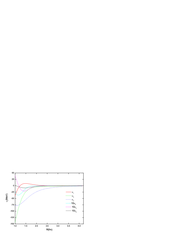
Figure 1: Various terms of the Skyrmion-antiSkyrmion potential potential Eq. (29). $\upsilon_{1}(R)$ is shown by the solid line, $\upsilon_{2}(R)$ by the dashed line, $\upsilon_{3}(R)$ by the dotted line, $\upsilon_{4}(R)$ by the dash-dotted line, $\upsilon_{5}(R)$ by the dash-dot-dotted line, and $\upsilon_{6}(R)$ by the short dash-dotted line.

Six independent choices of the matrix $C$ can yield enough independent linear equations to determine $\upsilon_{i}(R)(i=1-6)$ or equivalently $V_{i}(R)(i=1-6)$ through Eq. (30), and the numerical results for $\upsilon_{i}(R)(i=1-6)$ coming from the Mod-SKM are shown in Fig. 1. From this figure it can be seen that the first three term $\upsilon_{1}(R)$, $\upsilon_{2}(R)$ and $\upsilon_{3}(R)$ are dominant. It seems a good approximation to neglect the interaction terms which are nonlinear in the expansion of operator $W$ and $Z$. In the following discussion, we will mostly concentrate on the first three terms, then the leading term in this expansion is given by the following form:

$$V(\mathbf{R},C)=\upsilon_{1}(R)+\upsilon_{2}(R)W+\upsilon_{3}(R)Z$$ (31)

The algebraic operators $W$ and $Z$ have simple expectation values for the nucleons amado1

$$\langle N|T^{\alpha}_{pi}|N\rangle = -\frac{N_{C}}{3}P_{N}\langle N|\tau^{\alpha}_{p}\sigma^{\alpha}_{i}|N\rangle\;,$$

$$\langle N\overline{N}|W|N\overline{N}\rangle = \frac{1}{9}P^{2}_{N}\langle N\overline{N}|{\bm{\sigma}^{1}\cdot\bm{\sigma}^{2}\bm{\tau}^{1}\cdot\bm{\tau}^{2}}|N\overline{N}\rangle\;,$$

$$\langle N\overline{N}|Z|N\overline{N}\rangle = \frac{1}{9}P^{2}_{N}\langle N\overline{N}|(3\bm{\sigma}^{1}\cdot\mathbf{\hat{R}}\bm{\sigma}^{2}\cdot\mathbf{\hat{R}}-\bm{\sigma}^{1}\cdot\bm{\sigma}^{2})\bm{\tau}^{1}\cdot\bm{\tau}^{2}|N\overline{N}\rangle$$ (32)

Here $P_{N}$ is the finite $N_{C}$ correction factor $P_{N}=1+\frac{2}{N_{C}}$. By using Eq. (32) we take the $N\overline{N}$ matrix element of the interaction and evaluate the $N\overline{N}$ potential, which only contains three independent multipole component, i.e., the central part $V_{c}$, the spin-spin part $V_{s}$, and the tensor term $V_{t}$:

$$V^{(0)}(\mathbf{R})=V_{c}(R)+V_{s}(R)\bm{\sigma}^{1}\cdot\bm{\sigma}^{2}\bm{\tau}^{1}\cdot\bm{\tau}^{2}+V_{t}(R)(3\bm{\sigma}^{1}\cdot\mathbf{\hat{R}}\bm{\sigma}^{2}\cdot\mathbf{\hat{R}}-\bm{\sigma}^{1}\cdot\bm{\sigma}^{2})\bm{\tau}^{1}\cdot\bm{\tau}^{2}$$ (33)

with

$$V_{c}=\upsilon_{1}\;,~{}~{}~{}V_{s}=\frac{\upsilon_{2}P^{2}_{N}}{9}\;,~{}~{}~{}V_{t}=\frac{\upsilon_{3}P^{2}_{N}}{9}$$ (34)

The $N\overline{N}$ potential in the above is calculated by projecting Eq. (31) to the nucleon degrees of freedom only, and this is the correct procedure for large separation. However, at short distance the nucleons may deform or excite as they interact, and they can be virtually whatever the dynamics requires, for example, $\Delta(\rm{or}\;\overline{\Delta})$. This means that we need to consider the state mixing effect. In the case of $NN$ interaction, we saw that states mixing plays an important role in obtaining the phenomenologically correct potential. We expect the state mixing effect to be very important in the $N\overline{N}$ interaction as well. The state mixing comes into effect at the distance where the product ansatz makes no longer sense, so our results at short and intermediate distances should be suggestive, although we include state mixing. As a guide, we study the effects of the intermediate states $N\overline{\Delta}$, $\Delta\overline{N}$ and $\Delta\overline{\Delta}$ perturbatively, then to second order, the $N\overline{N}$ interaction is given by

$$V(\mathbf{R})=\langle N\overline{N}|V(\mathbf{R},C)|N\overline{N}\rangle+\sum_{s}\;^{\prime}\;\frac{\langle N\overline{N}|V(\mathbf{R},C)|s\rangle\langle s|V(\mathbf{R},C)|N\overline{N}\rangle}{E_{N\overline{N}}-E_{s}}$$ (35)

Here $E_{N\overline{N}}$ is the two nucleon energy and $E_{s}$ is the energy of the relevant excited state. The first term on the right is the direct nucleon-antinucleon projection of $V(\mathbf{R},C)$ and it is exactly the expression $V^{(0)}(\mathbf{R})$. The second term is the correction due to rotational or excited states. It is clear from the energy denominator that the second term is attractive. We need to evaluate the three sets of matrix elements $\langle N\overline{N}|V(\mathbf{R},C)|N\overline{\Delta}\rangle\langle N\overline{\Delta}|V(\mathbf{R},C)|N\overline{N}\rangle$, $\langle N\overline{N}|V(\mathbf{R},C)|\Delta\overline{N}\rangle\langle\Delta\overline{N}|V(\mathbf{R},C)|N\overline{N}\rangle$ and $\langle N\overline{N}|V(\mathbf{R},C)|\Delta\overline{\Delta}\rangle\langle\Delta\overline{\Delta}|V(\mathbf{R},C)|N\overline{N}\rangle$, and the final result for the first order correction to the $N\overline{N}$ interaction is nucleon5 ; amado2

$$V^{(1)}_{PT}(\mathbf{R})=-\frac{Q^{2}_{N}}{\delta}\{[\frac{1}{3}Q^{2}_{N}P^{\tau}_{0}+(\frac{16}{27}P^{2}_{N}+\frac{5}{27}Q^{2}_{N})P^{\tau}_{1}][\upsilon^{2}_{2}(R)+2\upsilon^{2}_{3}(R)]$$

$$+(\bm{\sigma}^{1}\cdot\bm{\sigma}^{2})[-\frac{1}{18}Q^{2}_{N}P^{\tau}_{0}+(\frac{16}{81}P^{2}_{N}-\frac{5}{162}Q^{2}_{N})P^{\tau}_{1}][\upsilon^{2}_{2}(R)-\upsilon^{2}_{3}(R)]+(3\bm{\sigma}^{1}\cdot\mathbf{\hat{R}}\bm{\sigma}^{2}\cdot\mathbf{\hat{R}}-\bm{\sigma}^{1}\cdot\bm{\sigma}^{2})$$

$$\times[-\frac{1}{18}Q^{2}_{N}P^{\tau}_{0}+(\frac{16}{81}P^{2}_{N}-\frac{5}{162}Q^{2}_{N})P^{\tau}_{1}][\upsilon^{2}_{3}(R)-\upsilon_{2}(R)\upsilon_{3}(R)]\}$$ (36)

Here $Q_{N}$ is another finite $N_{C}$ correction factor $Q_{N}=\sqrt{(1-1/N_{C})(1+5/N_{C})}$. $\delta$ is the $N-\Delta$ energy difference, which is about 300 MeV, and $P^{\tau}_{T}(T=0,1)$ is a projection operator onto the isospin $T$, $P^{\tau}_{0}=\frac{1}{4}(1-\bm{\tau}_{1}\cdot\bm{\tau_{2}})$, $P^{\tau}_{1}=\frac{1}{4}(3+\bm{\tau}_{1}\cdot\bm{\tau_{2}})$.

III.2 RESULTS

For each total isospin $T=0,1$ we parameterize the $N\overline{N}$ interaction potential by:

$$V^{T}_{N\overline{N}}=V^{T}_{c}+V^{T}_{s}\bm{\sigma}^{1}\cdot\bm{\sigma}^{2}+V^{T}_{t}(3\bm{\sigma}^{1}\cdot\hat{\mathbf{R}}\bm{\sigma}^{2}\cdot\hat{\mathbf{R}}-\bm{\sigma}^{1}\cdot\bm{\sigma}^{2})$$ (37)

We now calculate $V^{T}_{c}$, $V^{T}_{s}$, $V^{T}_{t}$ for each isospin $T$($T$=0,1) following the methods outlined above. Such a calculation requires considerable computing time. We would like to compare the Skyrmion model potentials with the realistic nucleon-antinucleon interaction potentials. However, we can not relate our results to the modern $N\overline{N}$ interaction potential such as the Paris potential paris and the Julich potential julich , since their central parts contain explicit momentum dependent terms. For that reason we compare our results with the phenomenological potentials of Bryan-Phillips bp and of the Nijmegen group nij . These potentials provide successful descriptions of both the $N\overline{N}$ scattering experiments data and the spectrum of resonances, and they are not qualitatively different from each other. At large distance all these potentials can be correctly described by the one-boson exchange mechanism and the $N\overline{N}$ potential can be obtained by $G$-parity transformation of the corresponding parts of the $NN$ interaction potential. Using equation of motion and the asymptotic form Eq. (6) of the chiral angle $F(r)$, the $N\overline{N}$ interaction based on the Mod-SKM tends to one pion exchange potential in the large distance region nucleon6 ,

$$V^{N\overline{N}}(r)\rightarrow\frac{-1}{4\pi}(\frac{g_{\pi NN}}{2M_{N}})^{2}(\bm{\tau}^{1}\cdot\bm{\tau}^{2})(\bm{\sigma}^{1}\cdot\bm{\nabla})(\bm{\sigma}^{2}\cdot\bm{\nabla})\frac{e^{-m_{\pi}r}}{r}~{}~{}~{}~{}(r\rightarrow\infty)$$ (38)

The parameters $e,F_{\pi},m$ are properly chose to guarantee that the long distance tail of the $N\overline{N}$ interaction will agree with the phenomenology. In order to model the annihilation effect at short distance, various cut off has been used in the Bryan-Phillips, Nijmegen, and other similar potentials. At short distance, the interaction is dominated by the strong absorptive potential of order 1 GeV, and it is significantly different from the meson exchange potential. Furthermore, the Skyrme model at short distance is no longer meaningful. so we should not take seriously the comparison of our results with the phenomenological potentials at 1 fm and less, however the results are still indicative at short distance. We find that the principal feature of the phenomenological $N\overline{N}$ interaction emerges from the careful calculation of that interaction based on the Mod-SKM, i.e., the strong central attraction.

Fig. 2 and Fig. 3 show the central potential $V^{T}_{C}$ calculated from Eq. (35) and the first term of the right hand of Eq. (35) only. In order to keep the figures clear, we plot the potential curves of $T=0$ and $T=1$ separately. For the case with the nucleon only, the results of $V^{T}_{C}$ are independent of the isospin $T$, and less attractive than the phenomenological potentials. When the perturbation corrections due to the effects of the intermediate states $N\overline{\Delta}$, $\Delta\overline{N}$ and $\Delta\overline{\Delta}$ (i.e., $\Delta$ mixing effects) are taken into account, the results of $V^{T}_{C}$ show significant attraction effects explicitly, and are closer to the Bryan-Phillips and Nijmegen potential. These perturbation results are rather realistic. The effects of $\Delta$($\overline{\Delta}$) mixing are so striking in the case of $T=1$ that the perturbation result is more attractive than the phenomenological potential for $T=1$. Furthermore, we would like to mention that, due to isospin conservation, the $N\Delta$ transition is missing in the $T=0$ channel which differentiates then the effect of the perturbation result between the $T=0$ and the $T=1$ channels. As a cross-check of our numerical calculation, we reproduce the results of Ref. amado2 , the nucleon only results of Ref. amado2 are also shown in Fig. 2 and Fig. 3 in order to illustrate the role of $B^{\mu}B_{\mu}$ term. From these figures it can be seen that the central potentials from the Mod-SKM are in better agreement with the phenomenology potentials.

In Fig. 4 and Fig. 5, we show the $T=0$ and $T=1$ spin-dependent potentials. In these cases the nucleon only potential and the perturbative results are quite similar. From 1 fm to about 1.5 fm, the potentials from the modified Skyrme model are not so close to the phenomenological potentials. Especially in the $T=0$ case, both the nucleon only and perturbative analysis give a positive spin-spin potential, in contrast to the negative values of the phenomenological potentials. It is important to see if the more complete Skyrme calculations can repair this disagreement. However, the smallness of the potential is reproduced. In our calculation, that small value arises from the cancelations of large terms.

Fig. 6 and Fig. 7 show the tensor potential $V^{T}_{t}$. Being similar to case of the spin-dependent potential, the nucleon only potential and the perturbative results are also quite similar. Particularly at large distance, these results agree with the phenomenological potential, but the agreement is not so good at intermediate distance. However, the difference between the theoretical and the phenomenological results is of the order of 10 MeV, compared to the static soliton mass or the nucleon mass which is about 1GeV, the difference is small enough. Here again, an improved Skyrme model dynamical calculation, going beyond the product ansatz, using diagonalization for state mixing and including explicitly the vector meson ($\rho,\omega$) and some high derivative terms in the Lagrangian, might lead to a better agreement.

IV conclusion and discussion

We have shown that the modified Skyrme model with product ansatz can give $N\overline{N}$ interaction which is in qualitatively agreement with the phenomenological potential, and it provides a better description of the static properties of single baryon than the minimal version Skyrme model. We see that the configuration mixing is very important to be included, and we roughly estimate this effect by perturbation theory. More sophisticated method of considering the state mixing effect is the Born-Oppenheimer approximation. The potential curves in the Born-Oppenheimer approximation are similar to the perturbative results, especially for the spin-dependent and the tensor potential nucleon5 ; amado2 .

To go from this work to a theory that can be confronted with experiment in detail is a difficult challenge, i.e, predicting the nucleon-antinucleon scattering cross section, the polarization, and the spectrums of the nucleon-antinucleon system etc. There are non-adiabatic effects that are particularly important at small $R$, and there are other mesons which should be included in the Skyrme lagrangian. The effects due to vector mesons may be particularly important at small distances. Obtaining the static nucleon-antinucleon interaction from Skyrme model based on large $N_{C}$ QCD can be a promising approach. We expect we can further discuss whether or not there exists nucleon-antinucleon bound state(baryonium) in this framework.

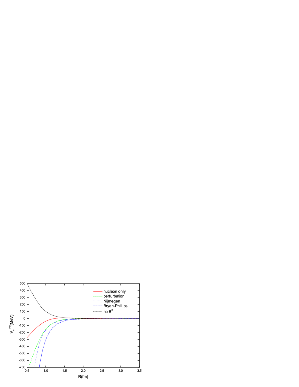
Figure 2: The central potential $V^{T}_{c}$ as a function of distance $R$ for the $T=0$ channel. The solid line is the nucleon only result, the dashed line is the result of the states mixing by perturbation theory. The dash-dot-dotted line is the nucleon only potential in conventional Skyrme model amado2 . The phenomenological potentials based on meson exchange are shown by dash-dotted line for the Bryan-Phillips potential and by dotted line for the Nijmegen potential.

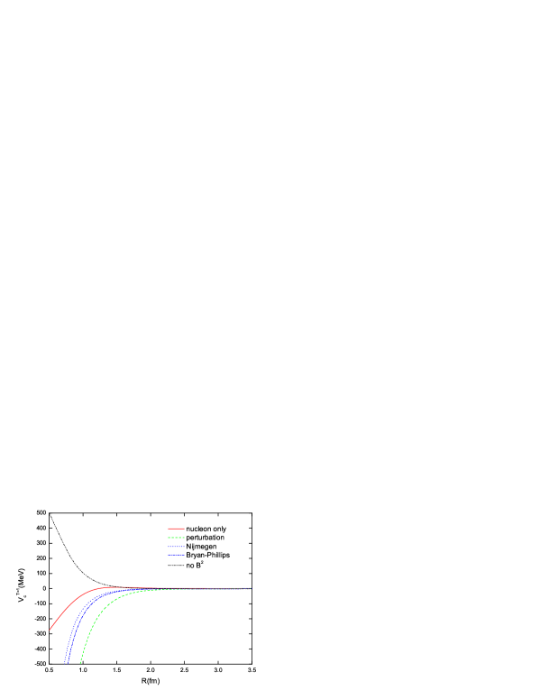
Figure 3: The central potential $V^{T}_{c}$ as a function of distance $R$ for the $T=1$ channel, labeling of the curves is the same as that in Fig. 2.

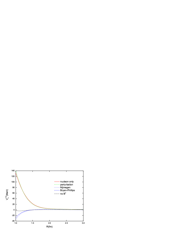
Figure 4: The spin-dependent potential $V^{T}_{s}$ as a function of distance $R$ for the $T=0$ channel, labeling of the curves is the same as that in Fig. 2.

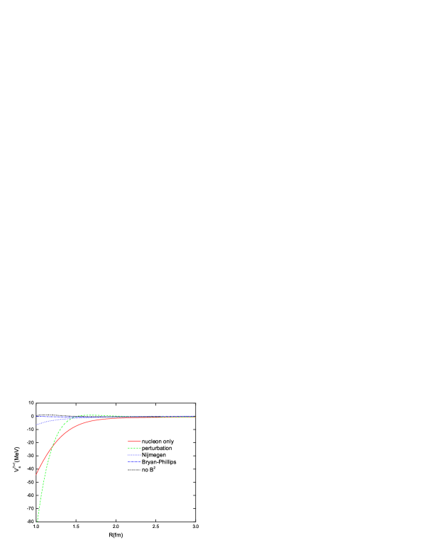
Figure 5: The spin-dependent potential, same as Fig. 4 but for $T=1$.

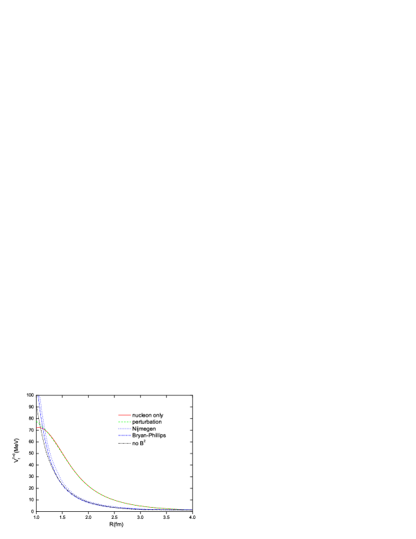
Figure 6: The tensor potential $V^{T}_{t}$ as a function of distance $R$ for the $T=0$ channel, labeling of the curves is the same as that in Fig. 2.

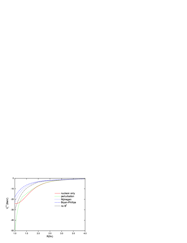
Figure 7: The tensor potential, same as Fig. 6 but for $T=1$

References

- (1) T.H.R.Skyrme, Proc. Roy. Soc. Lond. A 260, 127 (1961).
- (2) T.H.R.Skyrme, Nucl. Phys. 31, 556 (1962).
- (3) G. S. Adkins, C. R. Nappi and E. Witten, Nucl. Phys. B 228, 552 (1983).
- (4) G. S. Adkins and C. R. Nappi, Nucl. Phys. B 233, 109 (1984).
- (5) D. Diakonov, V. Petrov and M. V. Polyakov, Z. Phys. A 359, 305 (1997) [arXiv:hep-ph/9703373]; J. R. Ellis, M. Karliner and M. Praszalowicz, JHEP 0405, 002 (2004)[arXiv:hep-ph/0401127].
- (6) M.L.Yan, S.Li, B.Wu and B.Q.Ma, Phys. Rev. D 72, 034027 (2005).
- (7) G.J.Ding, M.L. Yan, Phys. Rev. C 72, 015208 (2005).
- (8) B. A. Li, M. L. Yan and K. F. Liu, Phys. Rev. D 43, 1515 (1991).
- (9) B. A. Li and M. L. Yan, Phys. Lett. B 282, 435 (1992).
- (10) D. Diakonov et al, Nucl. Phys. B480 341 (1996).
- (11) G. S. Adkins and C. R. Nappi, Phys. Lett. B 137, 251 (1984).
- (12) A. Jackson, A. D. Jackson and V. Pasquier, Nucl. Phys. A 432, 567 (1985).
- (13) R. Vinh Mau, M. Lacombe, B. Loiseau, W. N. Cottingham and P. Lisboa, Phys. Lett. B 150, 259 (1985); M. Lacombe, B. Loiseau, R. Vinh Mau and W. N. Cottingham, Phys. Lett. B 169, 121 (1986).
- (14) T. S. Walhout and J. Wambach, Phys. Rev. Lett. 67, 314 (1991).
- (15) A. Hosaka, M. Oka and R. D. Amado, Nucl. Phys. A 530, 507 (1991).
- (16) N. R. Walet and R. D. Amado, Phys. Rev. Lett. 68, 3849 (1992) [arXiv:nucl-th/9210015];Phys. Rev. C 47, 498 (1993).
- (17) H. Yabu and K. Ando, Prog. Theor. Phys. 74, 750 (1985).
- (18) M. Oka, R. Bijker, A. Bulgac and R. D. Amado, Phys. Rev. C 36, 1727 (1987).
- (19) Y. Lu and R. D. Amado, Phys. Rev. C 54, 1566 (1996)[arXiv:nucl-th/9606002].
- (20) Y. Lu, P. Protopapas and R. D. Amado, Phys. Rev. C 57, 1983 (1998)[arXiv:nucl-th/9710046].
- (21) BES Collaboration, J. Z. Bai et al., Phys. Rev. Lett. 91, 022001 (2003) [arXiv:hep-ex/0303006].
- (22) BES Collaboration, M. Ablikim et al., Phys. Rev. Lett. 95, 262001 (2005) [arXiv:hep-ex/0508025].
- (23) BES Collaboration, M. Ablikim et al., Phys. Rev. Lett. 93, 112002 (2004) [arXiv:hep-ex/0405050].
- (24) Belle Collaboration, K. Abe et al., Phys. Rev. Lett. 88, 181803 (2002) [arXiv:hep-ex/0202017].
- (25) Belle Collaboration, M. Z. Wang et al., Phys. Rev. Lett. 90, 201802 (2003) [arXiv:hep-ex/0302024].
- (26) Belle Collaboration, Y. J. Lee et al. , Phys. Rev. Lett. 93, 211801 (2004)[arXiv:hep-ex/0406068].
- (27) D. R. Entem and F. Fernandez, Phys. Rev. C 73, 045214 (2006).
- (28) G.J. Ding, J. l. Ping and M.L. Yan, Phys. Rev. D 74, 014029 (2006).
- (29) G. J. Ding and M. L. Yan, Eur. Phys. J. A 28, 351 (2006)[arXiv:hep-ph/0511186].
- (30) A. Jackson, A. D. Jackson, A. S. Goldhaber, G. E. Brown and L. C. Castillejo, Phys. Lett. B 154 (1985) 101.
- (31) M. Oka, Phys. Rev. C 36, 720 (1987).
- (32) R. Johnson, N. W. Park, J. Schechter, V. Soni and H. Weigel,Phys. Rev. D 42, 2998 (1990); A. Blotz, M. Praszalowicz and K. Goeke, Phys. Rev. D 53, 485 (1996)[arXiv:hep-ph/9403314]; G. Kaelbermann, J. M. Eisenberg and A. Schafer, Phys. Lett. B 339, 211 (1994)[arXiv:hep-ph/9409299].
- (33) J. Cote, M. Lacombe, B. Loiseau, B. Moussallam and R. Vinh Mau, Phys. Rev. Lett. 48, 1319 (1982); M. Pignone, M. Lacombe, B. Loiseau and R. Vinh Mau, Phys. Rev. C 50 (1994) 2710; B. El-Bennich, M. Lacombe, B. Loiseau and R. Vinh Mau, Phys. Rev. C 59 (1999) 2313.
- (34) T. Hippchen, J. Haidenbauer, K. Holinde and V. Mull, Phys. Rev. C 44, 1323 (1991).
- (35) R. A. Bryan and R. J. N. Phillips, Nucl. Phys. B 5, 201 (1968).
- (36) P. H. Timmers, W. A. van der Sanden and J. J. de Swart, Phys. Rev. D 29, 1928 (1984)[Erratum-ibid. D 30, 1995 (1984)].