Hadronization Approach for a Quark-Gluon Plasma Formed in Relativistic Heavy Ion Collisions

Abstract

A transport model is developed to describe hadron emission from a strongly coupled quark-gluon plasma formed in relativistic heavy ion collisions. The quark-gluon plasma is controlled by ideal hydrodynamics, and the hadron motion is characterized by a transport equation with loss and gain terms. The two sets of equations are coupled to each other, and the hadronization hypersurface is determined by both the hydrodynamic evolution and the hadron emission. The model is applied to calculate the transverse momentum distributions of mesons and baryons, and most of the results agree well with the experimental data at RHIC.

I Introduction

The hot and dense matter created in relativistic heavy ion collisions provides the condition to investigate the new state of matter of QCD, the so-called quark-gluon plasma(QGP) sign:intro1 ; sign:intro2 ; sign:itro_Rafelski_phL ; sign:EOS ; sign:intro3 . The space-time evolution of QGP and its hadronization process are still open questions in the research of this area. Hydrodynamics sign:hydro01 ; sign:hydro_Bro ; sign:hydro_Nonaka based on the assumption of local thermal and chemical equilibrium, models of quark coalescence or recombination sign:coal_1 ; sign:coal_2 ; sign:reco_rev ; sign:reco_1 ; sign:reco_2 ; sign:reco_S , and fragmentation sign:JetQuenchL1 ; sign:JetFrag1 are often used to describe the evolution and hadronization of QGP formed in heavy ion collisions at RHIC. However, we do not know a priori if the colliding system can reach equilibrium or not. In fact, because of the very small size and very short lifetime of the collision zone sign:finitesize1 ; sign:exp_HBT_STAR_200pion ; sign:hydro02 , the highly excited system may spend a considerable fraction of the lifetime in a non-equilibrium state sign:Hdr_expand . On the other hand, even if the system reaches equilibrium in the early quark-gluon stage, the hadrons formed in the later stage will be in non-equilibrium state, since the particle density in hadron phase is much smaller than that in the parton stage.

Evaporation models sign:Eva_eva ; sign:Eva_Cascade ; sign:Eva_eqi developed many years ago are widely used to describe the hadronization of QGP. In some of the models, the emission rate is calculated from a simple assumption of balance between the particle emission and absorption in QGP and in hadron gas at a critical temperature $T_{c}$. Under this assumption, the particle emission distribution is just the corresponding ideal thermal distribution of hadron gas, $f({\bf p})=f^{T}({\bf p})$.

However, considering the feedback effect of hadron evaporation on QGP, the space-time evolution of QGP and hadron evaporation are coupled to each other and the system is governed by both the hydrodynamic expansion and the evaporation. On the other hand, when the expansion of the system is fast, the fluid will be more likely to split into relatively small bubbles during the hadron evaporation. In this case, the system is a mixture of QGP bubbles and physical vacuum, and the energy density of the system is lower than that of a unitary QGP. These bubbles may provide a mechanism to reduce the viscosity of the system and make it more accessible for the ideal hydrodynamics to work at RHICsign:viscosityexp . Thirdly, from the analysis of collective flow measured at RHIC sign:Idealfluid , the QGP formed at RHIC is a strongly coupled quark-gluon plasma (sQGP) sign:diquark_baryon ; sign:sign bound_state ; sign:CSC1 ; sign:DiquarkRevIn where there exist not only quarks and gluons but also some of their resonant states like $qq$ and $qg$.

In this paper, we consider an effective hadronization model for the production of soft particles in relativistic heavy ion collisions. In the model, the QGP evolution is described by ideal hydrodynamics together with the equation of state including quarks, gluons and their resonant states. At the critical temperature, the expansion does not change the temperature of the system, and the decrease of the energy density is due to the splitting of the QGP fluid. When the energy density reaches the value for hadronization, which is a free parameter in our calculation, the evaporation starts and the hadron distributions are controlled by transport equations. The evaporation hypersurface is characterized by both the hydrodynamics and the evaporation.

The paper is organized as follows. In Section II we discuss hadron production and transport and derive an approximate emission distribution. In Section III we consider the hydrodynamics for the evolution of QGP with possible splitting into droplets and the effective evaporation boundary condition. We apply our model to hadron spectra in heavy ion collisions at RHIC energy in Section IV. We summarize in Section V.

II Hadron Emission

We investigate in this section the transport of hadrons emitted from QGP. The classical transport equation for the evolution of hadron phase space distribution $f(t,{\bf r},{\bf p})$ can be written as

$$\frac{\partial f}{\partial t}+{\bf v}\cdot\nabla f=Q+\alpha-\beta f,$$ (1)

where the second term on the left hand side is the free streaming part, and on the right hand side the lose and gain terms $\beta({\bf p})f$ and $\alpha({\bf p})$ indicate hadron absorption and production in QGP, and the elastic term $Q({\bf p};f)$ sign:R_Boltzmann1 controls the thermalization of the hadrons.

Under the assumption of quasi-static condition, the time evolution sign:R_Boltzmann2time during the transport can be temporarily removed. If we only focus on a one dimensional hadron transport in the region $x>0$ and treat the elastic scattering in relaxation time approximation, the hadron transport can be greatly simplified,

$${v\cos\theta}{\partial f\over\partial x}=-{f-f^{T}\over\tau}+\alpha-\beta f,$$ (2)

where $v=p/E$ is the hadron velocity, $\tau$ the relaxation time parameter, and $f^{T}(p)$ the thermal hadron distribution. In principle, $\tau$ should depend on the hadron momentum and the type of hadrons. For simplicity, we take it as a universal constant in our global model. Considering the finite volumes of hadrons and resonances, the phase space distribution will be suppressed. An effective way to include the volume effect in the thermal distribution is to multiply $f^{T}$ by a factor $1-y_{o}$, where $y_{o}$ is the ratio of the occupation volume of all the excluded hadrons to the whole volume of the system sign:vol_lit ; sign:VollEff . In the following calculation we will always consider this volume effect for $f^{T}$.

The transport equation (2) can be solved with the analytic result

$$f(x,\theta,p)=f_{\infty}(p)+\left[f(0,\theta,p)-f_{\infty}(p)\right]e^{-{\beta(p)\tau+1\over\tau v\cos\theta}x}$$ (3)

with $f_{\infty}(p)$ defined as

$$f_{\infty}(p)={f^{T}(p)+\alpha(p)\tau\over\beta(p)\tau+1}.$$ (4)

It is easy to see that the hadrons reach chemical equilibrium in the limit of vanishing inelastic interactions with $\alpha=\beta=0$ and thermal equilibrium in the limit of infinitely strong elastic interaction with $\tau=0$. In the both cases, the distribution at $x\to\infty$ is reduced to the thermal one,

$$f_{\infty}(p)=f^{T}(p).$$ (5)

Taking into account the boundary condition at $x=0$,

$$f(0,\theta,p)=0,\ \ \ \ (\cos\theta>0),$$ (6)

which means no hadrons moving from the vacuum in the region of $x<0$ to the QGP phase in the region of $x>0$, and the constraint

$$0\leq f(x,\theta,p)\leq f_{\infty}(p),$$ (7)

the hadron distribution can be expressed as

$$f(x,\theta,p)=f_{\infty}(p)\left[1-\Theta(\cos\theta)e^{-{\beta(p)\tau+1\over\tau v\cos\theta}x}\right],$$ (8)

where $\Theta(x)$ is a step function.

It can be seen from the above discussion that the influence of the transport process is mainly reflected in the region near the QGP surface at $x=0$. Most of the emitted hadrons are created in this region. Since the energy density in the inner part of the QGP fluid is higher than the value on the surface, the hadronization of the QGP fluid can be effectively regarded as a surface evaporation.

In the above derivation we did not consider the QGP surface shift and the breaking of the fluid in the process of hadron emission. A simple way to take the surface shift and fluid splitting into account is to introduce two parameters $v_{s}$ and $\eta$ in the model. The former is the shrinking velocity of the surface, and the latter is the ratio of the occupation volume of all the QGP droplets to the whole volume of the system. These two parameters should be considered simultaneously in the transport equation for hadron emission and the hydrodynamic equation for QGP evolution. With these two parameters, the hadron transport equation can be effectively written as

$$\left(v\cos\theta-v_{s}\right){\partial f\over\partial x}=\eta\left[-{f-f^{T}\over\tau}+\alpha-\beta f\right]$$ (9)

with the solution

$$f(x,\theta,p) = f_{\infty}(p)\times$$

$$\left[1-\Theta(v\cos\theta-v_{s})e^{-{\beta(p)\tau+1\over\tau(v\cos\theta-v_{s})}\int^{x}_{0}\eta(x^{\prime})dx^{\prime}}\right].$$

With the hadron distribution, the energy loss of the QGP fluid in the rest frame of the boundary can be expressed as

$${dE\over dtdS}=-\sum_{i}\int f^{i}_{\infty}(p_{i})\left(v_{i}\cos\theta-v_{s}\right)E_{i}d^{3}{\bf p}_{i},$$ (11)

where the integration over the angle $\theta$ is restricted by the condition $v_{i}\cos\theta-v_{s}<0$, $E_{i}$ is the energy of a hadron of type $i$, and the summation runs over all the hadron types. Similarly, the momentum loss of the QGP fluid can be written as

$${dP\over dtdS}=\sum_{i}\int f^{i}_{\infty}(p_{i})\left(v_{i}\cos\theta-v_{s}\right)p\cos\theta d^{3}{\bf p}_{i}.$$ (12)

If hydrodynamic expansion is neglected, the equation

$${dE\over dtdS}=\epsilon v_{s}$$ (13)

defines a minimal shrinking velocity of the fluid, where $\epsilon$ is the average energy density at the boundary. When $\epsilon$ is small enough to make $v_{s}=1$, the local association between different parts of the fluid will completely vanish, and the fluid must decouple. Therefore, the condition for the fluid description of the system is that the energy density must satisfy

$$\epsilon\geq\left.{dE\over dtdS}\right|_{v_{s}=1}.$$ (14)

The question left for the emission distribution of hadrons is the determination of the loss and gain terms $\beta$ and $\alpha$. We first calculate the absorption rate of hadrons by the medium. Considering that tens of kinds of hadrons will be discussed, the calculation of their different absorptions would be quite complicated. For simplicity, the inelastic absorption rate of a hadron by partons of type $j$ is described as

$$\beta_{j}({\bf p}) = \int g_{j}({\bf q})|{\bf v}-{\bf v}_{q}|\sigma_{j}({\bf p},{\bf q})d{\bf q}$$

$$= 4\pi\int q^{2}g_{j}(q)\sigma_{j}({\bf p},{\bf q})\frac{(v+v_{q})^{3}-|v-v_{q}|^{3}}{6vv_{q}}dq,$$

where $v_{q}=q/E$ denotes the parton velocity, $g_{j}$ is the parton thermal distribution at the critical temperature $T_{c}$ determined by the hydrodynamic equation, and $\sigma_{j}({\bf p},{\bf q})$ is the effective absorption cross section. Replacing $\sigma_{j}({\bf p},{\bf q})$ by its average value $\sigma_{j}$, we obtain the total absorption rate

$$\beta(p)=4\pi\sum_{j}{\sigma_{j}\zeta_{j}(p)}$$ (16)

with

$$\zeta_{j}(p) = \int_{0}^{\frac{m_{j}v}{\sqrt{1-v^{2}}}}\left[vg_{j}(q)q^{2}+{1\over 3v}g_{j}(q)\frac{q^{4}}{E_{j}^{2}}\right]dq$$ (17)

$$+\int_{\frac{m_{j}v}{\sqrt{1-v^{2}}}}^{\infty}\left[g_{j}(q)\frac{q^{3}}{E_{j}}+\frac{v^{2}}{3}g_{j}(q)qE_{j}\right]dq.$$

Since the diquark dynamics is not yet very clear, to simplify the calculation we take the assumption that the baryon cross section is $1.5$ times the meson cross section, $\langle\sigma_{b}\rangle=1.5\langle\sigma_{m}\rangle$.

For high momentum hadrons passing cold matter, we have

$$\zeta_{j}(p) \approx v\int_{0}^{\infty}{g_{j}(q)q^{2}dq}+\frac{1}{3v}\int_{0}^{\infty}{g_{j}(q)\frac{q^{4}}{E_{j}^{2}}dq}$$ (18)

$$= \frac{n_{j}}{4\pi}\left[v+\frac{1}{3v}\langle{v_{j}^{2}}\rangle\right],$$

where, $\langle{v_{j}^{2}}\rangle$ is a constant at given temperature and chemical potential, and $n_{j}$ is the parton density. In this case, the total rate can be approximately expressed as

$$\beta(p)\approx{v\over L},$$ (19)

where $L=1/\sum_{i}n_{j}\sigma_{j}$ is the inelastic mean free path.

For soft hadrons in hot medium, we have

$$\zeta_{j}(p) \approx \int_{0}^{\infty}{g_{j}(q)\frac{q^{3}}{E_{j}}dq}+\frac{v^{2}}{3}\int_{0}^{\infty}{g_{j}(q)qE_{j}dq}$$ (20)

$$= \frac{n_{j}}{4\pi}\left[\langle{v_{j}}\rangle+\frac{v^{2}}{3}\langle\frac{1}{v_{j}}\rangle\right].$$

Taking $\langle{v_{j}}\rangle=\langle\frac{1}{v_{j}}\rangle=1$ for gluons and light quarks and $\langle{v_{j}}\rangle\approx 0.96$ and $\langle\frac{1}{v_{j}}\rangle\approx 1.05$ for strange quarks with mass $m_{s}=95$ MeV, the total rate becomes approximately

$$\beta(p)\approx{1+v^{2}/3\over L}.$$ (21)

There are many mechanisms to describe hadron production in heavy ion collisions, such as two- or three-quark recombination for mesons or baryonssign:reco_1 ; sign:reco_2 ; sign:reco_S . In our model, there are not only quarks but also diquarks in the QGP. We assume that, mesons and intermediate baryons are respectively made of two quarks and one quark and one diquark, and final state baryons are considered as combinations of different intermediate baryon statessign:diquark_baryon , see Appendix A.

The produced hadron density in coordinate and time space through combination of two constituents $j$ and $k$ at a fixed channel $I$ can be defined as sign:crossection

$$n_{I}=\int|v_{j}-v_{k}|g_{j}({\bf p}_{j})g_{k}({\bf p}_{k})\sigma(p_{j},p_{k},p)d^{3}{\bf p}_{j}d^{3}{\bf p}_{k},$$ (22)

where $g_{j}$ and $g_{k}$ are the constituent distributions. and $\sigma$ is the cross section,

$$\sigma(p_{j},p_{k},p) = (2\pi)^{4}\int\frac{|M_{I}|^{2}}{4\sqrt{(p_{j}\cdot p_{k})^{2}-m_{j}^{2}m_{k}^{2}}}$$

$$\times\delta^{4}(p_{j}+p_{k}-p)\delta(p^{2}-m^{2})\Theta(E)\frac{d^{4}p}{(2\pi)^{3}}$$

with the scattering matrix element $M_{I}$.

For baryon production, since a diquark is much heavy than the corresponding quark, the hadron density can be approximately expressed as sign:diquark_baryon ; sign:diquark_Omega ,

$$n_{I}=2\pi^{3}|M_{I}|^{2}\int g_{j}(E_{j})g_{k}(E_{k})dE_{j}dE_{k},$$ (24)

where the integrated region is restricted by the constraints

$$m_{j} \leq {E_{j}}\leq{\infty},$$ (25)

$$E_{j}E_{k} \geq \frac{(E_{j}+E_{k})(m_{j}^{2}E_{k}+m_{k}^{2}E_{j})}{m^{2}}+E_{c}^{2},$$

$$E_{c} = {1\over 2m}\sqrt{\left[m^{2}-(m_{j}+m_{k})^{2}\right]\left[m^{2}-(m_{j}-m_{k})^{2}\right]}.$$

Since we have assumed thermalization of quarks, gluons and diquarks, their distribution functions can be written as

$$g_{j}({\bf p}_{j})=g_{j}(E_{j})=\frac{\kappa}{(2\pi)^{3}}\frac{\omega_{j}}{e^{\frac{E_{j}-\mu_{j}}{T_{c}}}\pm 1},$$ (26)

where $\omega_{j}=3J_{j}(J_{j}+1)$ is the degeneracy factor of spin and color degrees of freedom, and $\kappa$ is the reduction factor resulted from the volume effect of the bound-state or resonance-state components sign:VollEff ,

$$\kappa=\left[(1-y_{o})+C_{t}y_{o}\right]^{2-l}(1-y_{o})^{l},\\$$

with $l$ being the number of bound states or resonant states and $C_{t}$ the ”transparency” of bags. For simplicity, we set $C_{t}=1$.

Making summation over all the possible channels, we obtain the final hadron density

$$n=\sum_{I}C_{I}n_{I},$$ (27)

where $C_{I}$ is the weight factor of channel $I$ and is listed in Appendix A for different channels.

To have detailed information on the produced hadrons, we need the hadron momentum distribution

$${dn_{I}\over 4\pi{p^{2}}dp}={\pi^{2}\over 2}{|M_{I}|^{2}\over pE}\int F(E_{k})g_{j}(E-E_{k})g_{k}(E_{k})dE_{k},$$ (28)

where $F$ is defined as

$$F(E_{j})={\sqrt{EE_{k}(m^{2}-m_{j}^{2}+m_{k}^{2})-(E^{2}m_{k}^{2}+E_{k}^{2}m^{2})}\over mE_{c}},$$ (29)

and the integrated region is restricted by the constraint

$$E_{max} \leq E_{k}\leq E_{min},$$

$$E_{max} = Max\{m_{k},E_{-}\},$$

$$E_{min} = Min\{E-m_{j},E_{+}\},$$

$$E_{\pm} = {E\left(m^{2}-m_{j}^{2}+m_{k}^{2}\right)\pm 2mpE_{c}\over 2m^{2}}.$$ (30)

With the known produced hadron density, the gain term $\alpha$ in the transport equation (2) can be written as

$$\alpha(p)=\sum_{I}C_{I}\frac{dn_{I}}{(4\pi{p^{2}})dp}.$$ (31)

Note that in the calculation of lose and gain terms above, we considered only hadronization and hadron interactions with the QGP constituents. When the hadron decay in the transport process is included, it will certainly change the loss and gain terms. Its contribution to the production rate $\alpha$ will be effectively discussed in Section IV, and the change in the absorption rate $\beta$ can be described by a shift sign:PDG2006

$$\beta\to\beta+{\Gamma\over\gamma},$$ (32)

where $\Gamma$ is the hadron decay width and $\gamma$ is the Lorentz factor of the hadron.

In principle, all the particle masses are temperature and chemical potential dependent sign:Latt_CrossOver ; sign:TC1 . For quarks and gluons at the hadronization, we can simply take $m_{g}=0$, $m_{u}=3$ MeV, $m_{d}=6$ MeV and $m_{s}=95$ MeV sign:PDG2006 , but for light hadrons, their masses are in principle controlled by chiral symmetry and therefore deviate from their vacuum values. To simplify calculations, we will still use their masses and decay widths in the vacuum and neglect the medium effect. As for the diquark and $qg$ states, their masses in the vacuum sign:VollEff are taken as $m_{qq}=485$ MeV, $m_{qs}=580$ MeV in $0^{+}$ channel, $m_{qq}=725$ MeV, $m_{qs}=820$ MeV, $m_{ss}=905$ MeV in $1^{+}$ channel, and $m_{qg}=610$ MeV, $m_{sg}=715$ MeV in ${1\over 2}^{-}$ channel. These values are a bit smaller than the estimation in constituent quark model sign:Diquarkmassdef .

III QGP Evolution

We now turn to the space-time evolution of QGP. For ideal QGP, it can be described by the hydrodynamic equations,

$$\partial^{\mu}T_{\mu\nu}=0,\ \ \ \ \partial^{\mu}j_{\mu}^{i}=0,$$ (33)

where $T_{\mu\nu}=(\epsilon+P)u_{\mu}u_{\nu}-Pg_{\mu\nu}$ is the energy-momentum tensor of the fluid, $j^{i}_{\mu}=n_{i}u_{\mu}$ refers to the conserved charge current like baryon current and strange current, and $\epsilon,P,n_{i}$ and $u_{\mu}$ are respectively the energy density, pressure, conserved charge density and four velocity of the fluid.

To close the hydrodynamic equations, we need the equation of state of the fluid, $\epsilon(P)$. Since the parton fluid formed at RHIC energy is a strongly coupled QGP, we include in the equation of state the $u,d,s$ quarks, gluons, and all possible $qq$ and $qg$ resonant states. To simplify the calculation, we assume the relation $\epsilon=3P$ in the QGP stage.

From the hydrodynamic equation (33) and the equation of state, we can obtain the energy density $\epsilon$ as a function of space and time. When $\epsilon$ reaches $\epsilon_{c}$ corresponding to the critical temperature $T_{c}$ for deconfinement, the expansion of the system will no longer change the temperature, and the decrease of $\epsilon$ is assumed due to the splitting of the QGP fluid. Therefore, for the expansion process at fixed temperature $T_{c}$, the ratio of the energy densities $\epsilon/\epsilon_{c}$ is always less than $1$. Finally, when the energy density drops down to the value $\epsilon_{b}$ for the hadronization, which is a free parameter in our calculation, the hadron emission starts and the hydrodynamic evolution of the system becomes

$$\partial^{\mu}\left(T_{\mu\nu}-\overline{T}_{\mu\nu}\right)=0,\ \ \ \ \partial^{\mu}\left(j^{i}_{\mu}-\overline{j}^{i}_{\mu}\right)=0,$$ (34)

where $\overline{T}_{\mu\nu}$ and $\overline{j}^{i}_{\mu}$ are the changes in energy-momentum tensor and conserved charge current due to the hadron emission, and they are determined by the energy loss (11) and momentum loss (12). In this way, the evolution of the decoupling hypersurface of the fluid is determined by both the hydrodynamics and the evaporation, similar to the method in FCT calculations sign:hydro_cal1 ; sign:hydro_cal2 .

We discuss now, as an example, the spherical expansion of hydrodynamics to demonstrate the influence of evaporation on the hadronization boundary. The $1+1$ hydrodynamics of QGP can be written as sign:hydro_t_3 ,

$${\partial\xi\over\partial t} = -\frac{2}{3-v^{2}}\left[v{\partial\xi\over\partial r}+2{\partial v\over\partial r}+2(N-1){v\over r}\right],$$

$${\partial v\over\partial t} = -{1\over 3-v^{2}}\bigg{[}{3(1-v^{2})^{2}\over 4}{\partial\xi\over\partial r}+2v{\partial v\over\partial r}$$

$$\ \ \ \ \ \ \ \ -(N-1){v^{2}(1-v^{2})\over r}\bigg{]},$$

$${\partial n_{\gamma}\over\partial t} = -\left[v{\partial n_{\gamma}\over\partial r}+n_{\gamma}{\partial v\over\partial r}+(N-1)n_{\gamma}{v\over r}\right]$$ (35)

for the spherical hydrodynamic velocity $v$, the scaled energy-momentum quantity $\xi=\ln\left[(\epsilon+P)/(\epsilon_{b}+P_{b})\right]$, and the conserved charge density $n_{\gamma}=n_{B}\gamma$, where $\gamma$ is the Lorentz factor of the fluid, $n_{B}$ is the baryon density, and $N=3$ is the symmetric dimension.

Similarly, we can derive the simplified 1+1 hydrodynamic equation including the feedback from the hadron evaporation. When $\epsilon$ calculated from the hydrodynamics with evaporation is less than $\epsilon_{b}$, the hadronization hypersurface is determined by (III). Otherwise, the hydrodynamics with evaporation itself gives the hypersurface.

The radius $R$ of the hadronization spherical surface, the hydrodynamic expansion velocity $v$ on the surface, and the bulk energy of the fluid are shown as functions of time in Fig.1 for different values of shrinking velocity $v_{s}$ which characterizes the effect of hadron emission on the shift of hydronization hypersurface. In the calculation, we have chosen the initial energy density distribution as a Gaussian distribution with the central value $\epsilon(r=0)=9\epsilon_{b}$ and the initial expansion velocity $u(r)=\gamma v=0.05r\ fm^{-1}$. For $v_{s}=0$ which means no hadron emission, the radius and the expansion velocity are fully determined by the hydrodynamic equations (III). With increasing hadron emission, the shrinking velocity increases, and the hadronization radius, the expansion velocity and the bulk energy deviate from the pure hydrodynamic solution more and more strongly. Since the hydrodynamic expansion grows with increasing time, the quantities are always controlled by the pure hydrodynamics and the emission effect can be neglected in the later stage of the fluid.

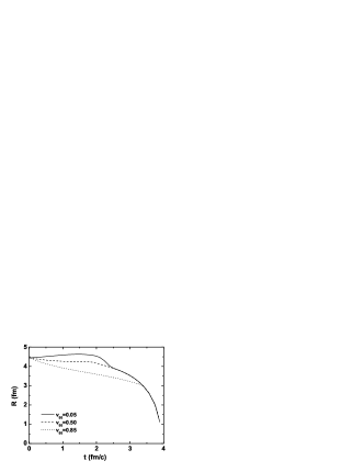
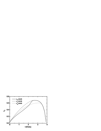
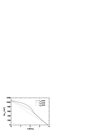
Figure 1: The hadronization radius $R$, the expansion velocity $v$ at the radius, and the bulk energy $E$ scaled by the hadronization energy density $\epsilon_{b}$ of the QGP fluid as functions of time for several values of shrinking velocity $v_{s}$, calculated in the frame of spherical expansion.

To study the space-time evolution of relativistic heavy ion collisions at RHIC energy, it is better to consider the cylindrical expansion of hydrodynamics. As is usually done, the longitudinal expansion can be decoupled from the transverse expansion and described in the Bjorken boost invariant scenario sign:bjorken . The transverse expansion is described by equation (III) with $N=2$. As an example, we consider a central Au-Au collision at colliding energy $\sqrt{s}=200$ GeV. The initial condition of the collision, which is the same as in sign:hydro01 ; sign:hydro02 , is determined by the nuclear geometry sign:hydro_Glauber and the corresponding nucleon-nucleon interaction. The formation time of the locally thermalized fluid is set to be $\tau_{0}=0.6$ $fm/c$.

The hadronization radius $R$ in the transverse plane and the corresponding expansion velocity $v$ at $R$ are shown in Fig.2. The hadronization energy density is chosen as $\epsilon_{b}=0.21$ GeV/fm³ by fitting the RHIC data, and the shrinking velocity $v_{s}$ is the maximum of its value solved from the self-consistent equations (11) and (13) for the emission energy and its value determined from the QGP hydrodynamic equation with splitting. Different from the spherical expansion where the hadron emission plays an essential role in determining the hadronization radius, the evaporation in the frame of cylindrical expansion does not change the pure hydrodynamic result considerably, except in the very beginning period. This behavior is due to the rapid expansion in the Bjorken scenario.

Figure 2: The hadronization radius $R$ and the corresponding expansion velocity $v$ of the QGP fluid as functions of time in a central Au-Au collision with colliding energy $\sqrt{s}=200$ GeV per pair of nucleons, calculated in the frame of cylindrical expansion.

IV Hadron Production at RHIC

Now it is the time for us to apply our model with hydrodynamics for QGP evolution and transport for hadron emission to relativistic heavy ion collisions. We will calculate the spectra of soft hadrons produced in central Au-Au collisions at colliding energy $\sqrt{s_{NN}}=200$ GeV and compare the results with experimental data at RHIC sign:exp_PHENIX_ppik ; sign:exp_PHOBOS_pi ; sign:exp_STAR_ppik2006 ; sign:exp_STAR_StrangeOld ; sign:exp_STAR_Strange ; sign:exp_STAR_Strange2 ; sign:exp_STAR_K892 ; sign:exp_STAR_phi ; sign:exp_PHENIX_phi ; sign:exp_STAR_Sig1385 ; sign:exp_STAR_Xi1530 ; sign:exp_Ratio_Omegaphi ; sign:exp_Ratio_STAR_Omega .

Let’s first list the free parameters in the model. We choose the critical temperature $T_{c}=166$ MeV which leads to the critical energy density $\epsilon_{c}=1.91$ GeV/fm³. Since resonant states of $qq$ and $qg$ are taken into account in our equation of state for the strongly coupled QGP, the energy density is larger than the Stefan-Boltzmann limit for the ideal system of quarks and gluons, $\epsilon_{c}=1.24\epsilon_{SB}$. The average cross section for meson-quark inelastic scattering is taken to be $\langle\sigma_{m}\rangle=7$ mb. The ratio $y_{o}$ to describe the finite volume effect of hadrons is taken as $0.83$. From our numerical calculation, the obtained hadron spectra are not sensitive to the value of $y_{o}$ in a wide region. To minimize the free parameters, we assume that the hadrons are not thermalized at all, namely we take the relaxation time $\tau=\infty$ for all hadrons. In this case, the hadron distribution is controlled only by the emission rate and medium absorption,

$$f_{\infty}(p)={\alpha(p)\over\beta(p)}.$$ (36)

Further more, by fitting the PHENIX data sign:exp_PHENIX_ppik of protons and pions, we determine the energy density of the QGP fluid $\epsilon_{b}=0.21$ GeV/fm³ at hadronization which corresponds to the ratio $\eta=\epsilon_{b}/\epsilon_{c}=0.11$, the chemical potential $\mu_{B}=27$ MeV at hadronization, and the meson-quark and baryon-quark coupling constants $g_{M}^{2}=5.11$ and $g_{B}^{2}=34.24$. For strange quark $s$, its chemical potential is $\mu_{s}=\mu_{B}/3-\mu_{S}$ where $\mu_{S}$ is the strange chemical potential. With the above parameters, the evolution duration of the QGP fluid, calculated from the hydrodynamic equation, is about $8.4$ fm/c.

The invariant yields of hadrons with type $i$ can be calculated from the phase space integration of the hadron distribution

$$\frac{d^{2}N_{i}}{2\pi p_{T}dp_{T}dy} = \frac{d}{2\pi p_{T}dp_{T}}\sum_{j}\int f^{j}_{\infty}({\bf q}^{\prime})\left(v^{\prime}_{j}\cos\theta-v^{\prime}_{s}\right)$$ (37)

$$\times F_{D}^{ji}({\bf q},{\bf p})d^{2}{\bf x}dt^{\prime}d^{3}{\bf q^{\prime}},$$

where $F_{D}^{ji}$ stands for the decay from hadrons of type $j$ to the hadrons of type $i$, ${\bf q}^{\prime}$ is the hadron momentum in the local rest frame of the hadronization hypersurface and is related to the momentum ${\bf q}$ by a Lorentz transformation. It is necessary to note that, the decay contribution to the gain term $\alpha$, mentioned in the last section, can be effectively described by multiplying the decay term $F_{D}^{ji}$ here by a factor

$$\alpha_{ji}=1+\xi_{j+1,j}+\xi_{j+1,j}\xi_{j+2,j+1}+\cdots+\xi_{j+1,j}\cdots\xi_{i,i-1},$$ (38)

with

$$\xi_{j+1,j}={\Gamma_{j}/\left(\gamma_{j}\eta\right)\over\beta_{j+1}+\Gamma_{j+1}/\left(\gamma_{j+1}\eta\right)},$$ (39)

where we have considered the assumption of $\tau=\infty$.

The phase space integration is done by a Monte-Carlo simulation, which partially trace the directly emitted hadrons. By counting enough events, the statistical error for $dN/dy$ caused by the random simulation is less than $0.5\%-1\%$ for different hadrons. The statistical error for $p_{T}$ distribution is, however, relatively larger, especially in very low $p_{T}$ and high $p_{T}$ regions. The reason is the denominator $p_{T}$ in (37) for low $p_{T}$ hadrons and low abundance for high $p_{T}$ hadrons. In the region of $p_{T}=0.3-4$ GeV, the statistical error is expected to be smaller than $5\%$ for most hadrons.

The light hadron yield is dominated by decay product. For example, the number of direct pions is less than $5\%$ of the total final state pion abundance. Since the convergence of heavy resonance decay contribution is slow, many resonances need to be considered in our calculations. The selection of hadron types is subject to their relative production rates and branch ratios, compared with their daughter particles counted in our calculations. Mesons and baryons included in our model are listed in Table 1 and 2. Although some of $0^{+}$ particles, such as $f_{0}(600)$, $f_{0}(980)$ and $a_{0}(980)$ are often interpreted as non-$q\bar{q}$ states, they are still treated as scalar mesons in our calculations.

$0^{-}$	$1^{-}$	$0^{+}$	$1^{+}$	$2^{+}$
$\pi$	$\rho$	$a_{0\;980}$	$b_{1\;1235}$	$K_{2\;1430}$
$K$	$K^{*}_{\;892}$	$f_{0\;600}$	$h_{1\;1170}$
$\eta$	$\omega$	$f_{0\;980}$	$a_{1\;1260}$
$\eta^{\prime}$	$\phi$	$K_{0\;1430}$	$f_{1\;1285}$
	$K^{*}_{\;1410}$		$K_{1\;1270}$
			$K_{1\;1400}$

Table 1: Mesons selected in the calculations.

$N$	$\Delta$	$\Lambda$	$\Sigma$	$\Xi$	$\Omega$
$N_{938}$	$\Delta_{1232}$	$\Lambda_{1116}$	$\Sigma_{1192}$	$\Xi_{1317}$	$\Omega_{1672}$
$N_{1440}$	$\Delta_{1600}$	$\Lambda_{1405}$	$\Sigma_{1385}$	$\Xi_{1530}$
$N_{1520}$	$\Delta_{1620}$	$\Lambda_{1520}$	$\Sigma_{1660}$	$\Xi_{1690}$
$N_{1535}$		$\Lambda_{1600}$	$\Sigma_{1670}$	$\Xi_{1820}$
		$\Lambda_{1670}$	$\Sigma_{1750}$
		$\Lambda_{1690}$	$\Sigma_{1775}$
		$\Lambda_{1830}$

Table 2: Baryons selected in the calculations.

The hadron spectra and relative ratios are calculated with the invariant momentum distribution (37) at $y=0$. Since the data for exclusive protons and inclusive pions from PHENIX sign:exp_PHENIX_ppik are used to fit the parameters, the agreement between our model calculation and the data for these two kinds of particles, shown in Figs.3, 4 and 5, looks perfect.

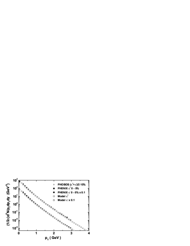
Figure 3: The transverse momentum distributions of $\pi^{\pm}$. The abundances are inclusive, and no feed-down corrections are applied. The data are from PHENIX sign:exp_PHENIX_ppik and PHOBOS sign:exp_PHOBOS_pi Collaborations.

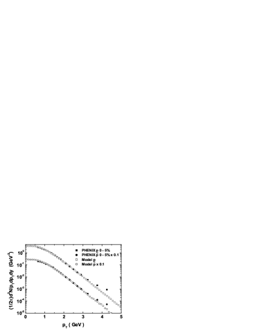
Figure 4: The transverse momentum distributions of protons and anti-protons. The feed-down corrections from $\Lambda$ are applied. The data are from PHENIX Collaboration sign:exp_PHENIX_ppik .

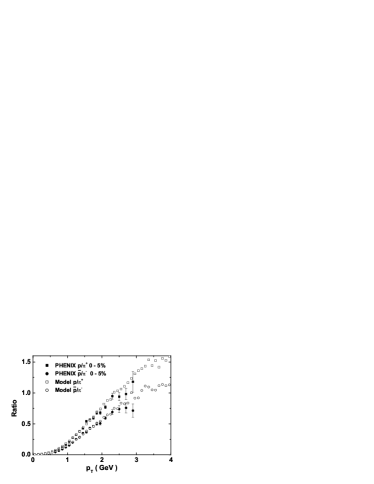
Figure 5: The $p/\pi^{+}$ and $\bar{p}/\pi^{-}$ ratios as functions of transverse momentum. The data are from PHENIX Collaboration sign:exp_PHENIX_ppik .

As only soft particles are emitted from the QGP fluid itself, the hadron spectra in high transverse momentum region are expected not to be reproduced correctly in our model. For these high $p_{T}$ particles, we should consider the jet motion in QGP and its fragmentation mechanism. The effect of jets or shower partons in high $p_{T}$ region is more significant for pions and protons, compared with those heavy resonances, especially multi-strange heavy resonances. The big difference between our model calculation and STAR data sign:exp_STAR_ppik2006 for high $p_{T}$ pions and protons is shown clearly in Figs. 6 and 7.

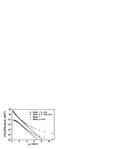
Figure 6: The transverse momentum distributions of proton and $\pi^{+}$. The distribution for proton is inclusive, and the decay contribution from $\Lambda$ and $K^{0}_{S}$ to pions is removed. The data are from STAR Collaboration sign:exp_STAR_ppik2006 .

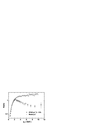
Figure 7: The $p/\pi^{+}$ ratio as a function of transverse momentum. The distribution for proton is inclusive, and the decay contribution from $\Lambda$ and $K^{0}_{S}$ to pions is removed. The data are from STAR Collaboration sign:exp_STAR_ppik2006 .

The transverse momentum distributions for charged kaons are shown in Fig. 8. Our model result looks higher than the experimental data. The reason is probably the lack of heavy resonances in our hadron list or the light strange quark with $m_{s}=95$ MeV sign:PDG2006 . A heavier strange quark can reduce the production of strange hadrons like kaons, $\Sigma^{*}(1385)$ and $\Xi^{*}(1530)$. For $m_{s}=170$ MeV, the suppression for kaons is about $5\%$. Another possible reason for the overestimation of kaons is the strange hadron thermalization. If we take the relaxation time $\tau\sim 1$ fm, the model calculation agrees well with the data.

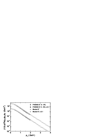
Figure 8: The transverse momentum distributions of $K^{\pm}$. The abundances are inclusive and no feed-down corrections are applied. The data are from PHENIX Collaboration sign:exp_PHENIX_ppik .

The $\Lambda$ and $\Xi^{-}$ spectra are shown in Figs. 9 and 10. The model describes well the $\Xi$ data, but the result deviates from the data for $\Lambda$ and $\bar{\Lambda}$ remarkably in low $p_{T}$ region, especially for the positive $\Lambda$. Compared with the experimental data, a general behavior of our model calculation is the enhancement of strange mesons and suppression of strange baryons. This is probably due to the exclusion of the hadron rescattering, such as $N+\bar{K}\leftrightarrows\Sigma(\Lambda)+\pi$ or $N+\bar{K}\rightarrow\Sigma^{*}(\Lambda^{*})+X$, or the treatment of diquarks. In our current frame, diquarks are thermalized like quarks and gluons and satisfy the Bose-Einstein distribution. Since diquarks are so heavy, it is more reasonable to describe their phase-space distribution by a transport equation, like the one for hadrons.

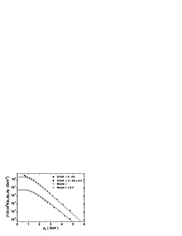
Figure 9: The transverse momentum distributions of $\Lambda$ and $\Xi^{-}$. The decay contribution from $\Xi^{-}$, $\Xi^{0}$ and $\Omega$ to $\Lambda$ is removed, but the one from $\Sigma^{0}$ is included. The distribution for $\Xi^{-}$ is inclusive. All the data are from STAR Collaboration sign:exp_STAR_StrangeOld ; sign:exp_STAR_Strange .

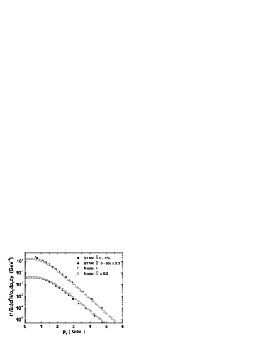
Figure 10: The transverse momentum distributions of $\bar{\Lambda}$ and $\bar{\Xi}^{+}$. The treatment for decay contribution is the same as in Fig.9. The data are from STAR Collaboration sign:exp_STAR_StrangeOld ; sign:exp_STAR_Strange .

The transverse momentum distributions for $\Lambda,K^{+}$ and $K^{0}_{S}$ and the ratio $\Lambda/K_{S}^{0}$ are shown in Figs. 11 and 12. Again we see clearly the theoretical enhancement for $K$ and suppression for $\Lambda$. From the comparison with the STAR data, the inclusive $\Lambda$ distribution without the feed-down correction seems much better than the one shown in Fig.9. Different from the theoretical soft $p/\pi$ ratio shown in Fig.7 where the ratio never decreases, the soft $\Lambda/K$ ratio begins to drop down at about $p_{T}\sim 4$ GeV.

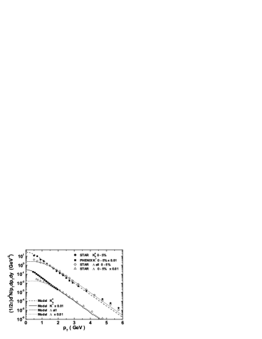
Figure 11: The transverse momentum distributions of ${\Lambda},K^{+}$ and $K^{0}_{S}$. The distributions for $K^{0}_{S}$ and ”$\Lambda$ $all$” are inclusive, and the other decay treatment is the same as in Fig.9. All the data are from STAR Collaboration sign:exp_PHENIX_ppik ; sign:exp_STAR_StrangeOld ; sign:exp_STAR_Strange ; sign:exp_STAR_Strange2 .

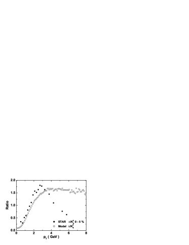
Figure 12: The ratio $\Lambda/K^{0}_{S}$ as a function of transverse momentum. The abundances are inclusive, and no feed-down correction is applied. The data are from STAR Collaboration sign:exp_STAR_Strange2 .

The $K^{*}(892)$ yield is shown in Fig. 13 as a function of $m_{T}-m_{K^{*}}$, where $m_{T}=\sqrt{p_{T}^{2}+m_{K^{*}}^{2}}$ is the particle transverse mass. From the comparison with the STAR data, the decay correction from the loss term (32) plays an important role. As the decay products may be absorbed by the medium, or their momenta may be shifted, it is hard to obtain the reconstruction. Since the meson inelastic cross section is supposed to be $2/3$ of the baryon cross section, the contribution from ITD loss for mesons would be more significant than the one for baryons. The transverse momentum distributions for $\rho^{0}$ and $\omega$ are predicted in Fig. 14.

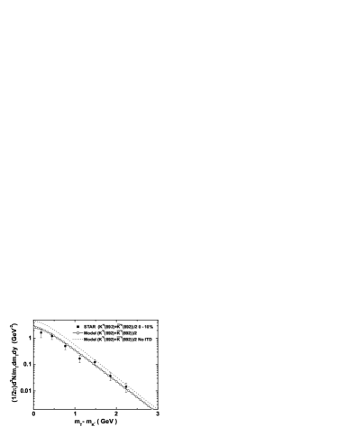
Figure 13: The inclusive $m_{T}$ distribution of $(K^{*0}(892)+\overline{K}^{*0}(892))/2$. The dotted line is the model calculation without considering the in-transport decay (ITD) loss correction. The data are from STAR Collaboration sign:exp_STAR_K892 .

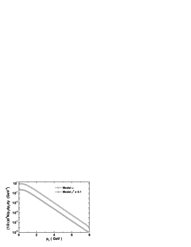
Figure 14: The model predicted inclusive distributions of $\rho^{0}$ and $\omega$.

The $\phi$ production is shown in Fig.15. The model results are much larger than the experimental data. This is partially due to the limited hadron list in our treatment. Otherwise, the emission at the hypersurface for $\phi$ may not be effective. Note the fact that the STAR data sign:exp_STAR_phi are about twice the PHENIX data sign:exp_PHENIX_phi , further precise measurement for $\phi$ is required.

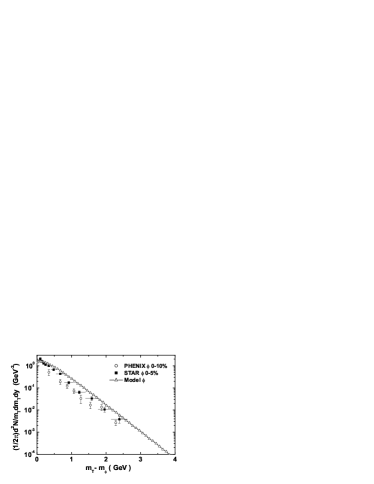
Figure 15: The inclusive $m_{T}$ distribution of $\phi(1020)$. The $x$ error bar is used here to show the $m_{T}$ bin size. The data are from STAR sign:exp_STAR_phi and PHENIX sign:exp_PHENIX_phi Collaborations.

The $\Sigma^{*}(1385)$ distribution is shown in Fig. 16. The model results are much smaller than the experimental data, especially in very low $p_{T}$ region. The situation here is similar to the case for $\Lambda$. The $\Lambda\pi$ or $N\bar{K}$ process which is excluded in the model may regenerate some $\Sigma^{*}(1385)$ sign:exp_STAR_Sig1385 ; sign:exp_STAR_Xi1530 . As $\Sigma^{*}(1385)$ can not decay to $N\bar{K}$ due to its low mass, it may become a one-way valve to deliver strange quarks from $K$ to $\Lambda(\Sigma)$. Another possible reason for the $\Sigma^{*}$ suppression is that many heavy resonances which would decay to $\Sigma^{*}(1385)$ are not included in our calculation.

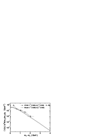
Figure 16: The inclusive $m_{T}$ distribution of $\Sigma^{*\pm}(1385)+\overline{\Sigma}^{*\mp}(1385)$. The data are from STAR Collaboration sign:exp_STAR_Sig1385 .

The transverse momentum distributions of $\Xi^{*0}(1530)$ and $\Omega$ are shown in Fig.17. For $\Omega$, the calculated distribution is close to the data in low $p_{T}$ region but deviate from the data in high $p_{T}$ region. The situation is similar to $\phi$. This shows that either more resonances should be considered or the scenario of the hypersurface emission for these hadrons need to be corrected. From the data, it looks that there are two slope parameters for $\Omega$, like $\Lambda$ and $\Sigma^{*}(1385)$. As for $\Xi^{*0}(1530)$, the model calculation is bad at low $p_{T}$. It might be due to the fact that $\Xi(1950)$ is not counted in our model. $\Xi(1950)$ is a mysterious baryon. Its spin, parity and branch ratios are not clear, and it is even suggested that there might be more than one $\Xi$ at that mass sign:PDG2006 .

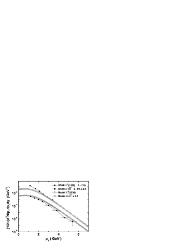
Figure 17: The inclusive transverse momentum distributions of $\Xi^{0}(1530)$ and $\Omega^{-}+{\bar{\Omega}}^{+}$. The data are from STAR Collaboration sign:exp_STAR_Xi1530 ; sign:exp_STAR_StrangeOld ; sign:exp_STAR_Strange .

The ratio of $\Omega$ to $\phi$ is presented in Fig.18 as a function of transverse momentum. As multi-strange hadrons, the jet contribution to $\phi$ and $\Omega$ is expected to be small, as we have seen in their spectra in Figs.15 and 17. Our results are similar to the ones calculated in recombination model sign:reco_S .

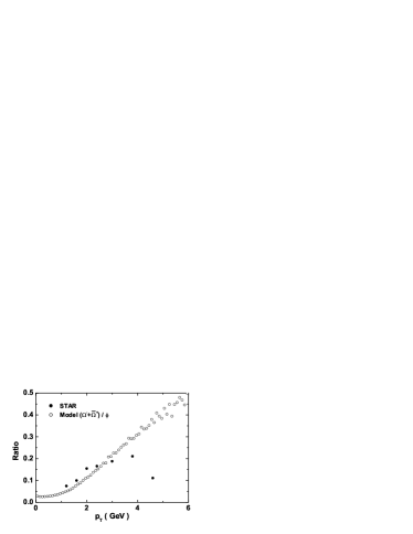
Figure 18: The inclusive ratio $(\Omega^{-}+{\bar{\Omega}}^{+})/\phi$ as a function of transverse momentum. The data are from STAR Collaboration sign:exp_Ratio_Omegaphi .

Some of the momentum integrated ratios are listed in Table 3 and compared with experimental data sign:exp_PHENIX_ppik ; sign:exp_Ratio_STAR_Omega . The data from sign:exp_Ratio_STAR_Omega correspond to baryons in the $p_{T}$ region of $2.4-3.6$ GeV and mesons in the $p_{T}$ region of $1.6-2.4$ GeV. The influence of hadron decay is relatively small in these regions. The strange baryon ratios at colliding energy $\sqrt{s}=200$ GeV sign:exp_Ratio_STAR_Omega are very similar to the data at energy $\sqrt{s}=130$ GeV sign:sign harris ; sign:sign Lambda_STAR ; sign:sign Lambda_PHENIX . Some meson and baryon ratios as functions of transverse momentum are shown in Figs.19 and 20.

$Particles$	$Model$		$\qquad Exp$
$\pi^{-}/\pi^{+}$(in)	1.006		$0.984\pm 0.004\pm 0.057$ sign:exp_PHENIX_ppik
$\pi^{-}/\pi^{+}$(ex)	0.999		$1.01\pm 0.02$ sign:exp_Ratio_STAR_Omega
$K^{-}/K^{+}$	0.915		$0.933\pm 0.007\pm 0.054$ sign:exp_PHENIX_ppik
			$0.96\pm 0.03$ sign:exp_Ratio_STAR_Omega
$\bar{p}/p$(ex)	0.748		$0.731\pm 0.011\pm 0.062$ sign:exp_PHENIX_ppik
$\bar{p}/p$(in)	0.783		$0.747\pm 0.007\pm 0.046$ sign:exp_PHENIX_ppik
			$0.77\pm 0.05$ sign:exp_Ratio_STAR_Omega
$\overline{{\Lambda}}/\Lambda$	0.844		$0.72\pm 0.024$ sign:exp_Ratio_STAR_Omega
$\overline{\Xi}^{+}/\Xi^{-}$	0.907		$0.82\pm 0.05$ sign:exp_Ratio_STAR_Omega
$\overline{\Omega}^{+}/\Omega^{-}$	1.011		$1.01\pm 0.08$ sign:exp_Ratio_STAR_Omega
$K^{+}/\pi^{+}$	0.203		$0.171\pm 0.001\pm 0.010$ sign:exp_PHENIX_ppik
$K^{-}/\pi^{-}$	0.184		$0.162\pm 0.001\pm 0.010$ sign:exp_PHENIX_ppik
$p_{{}_{ex}}/\pi^{+}$	0.0645		$0.064\pm 0.001\pm 0.003$ sign:exp_PHENIX_ppik
$p/\pi^{+}$(in)	0.102		$0.099\pm 0.001\pm 0.006$ sign:exp_PHENIX_ppik
$\bar{p}_{{}_{ex}}/\pi^{-}$	0.0479		$0.047\pm 0.001\pm 0.002$ sign:exp_PHENIX_ppik
$\bar{p}/\pi^{-}$(in)	0.0797		$0.075\pm 0.001\pm 0.004$ sign:exp_PHENIX_ppik

Table 3: Some momentum integrated hadron ratios compared with RHIC data sign:exp_PHENIX_ppik ; sign:exp_Ratio_STAR_Omega . The statistical errors in the model calculations are up to $5\%$.

Figure 19: The inclusive $\pi^{-}/\pi^{+}$ and exclusive $\bar{p}/p$ ratios as functions of transverse momentum. The data are from PHENIX Collaboration sign:exp_PHENIX_ppik .

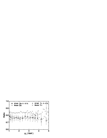
Figure 20: The inclusive $\bar{p}/p$ and $\bar{\Lambda}/\Lambda$ ratios as functions of transverse momentum. The data are from STAR Collaboration sign:exp_STAR_ppik2006 ; sign:exp_STAR_Strange2 .

$\Sigma^{0}$ and $\Lambda$ particles are sensitive to the hadronization mechanisms. In some string fragmentation models the ratio $\Sigma^{0}/\Lambda$ is taken to be $\sim 0.35$, but in thermal statistical models it is predicted to be $0.65-0.75$ due to the mass difference. If the hadronization is dominated by gluon junction or coalescence, the ratio is about $1$. In our case, the hadronization mechanism is similar to the coalescence or recombination, but the ratio is a little larger than $1$ sign:diquark_baryon ; sign:diquark_Omega . The reason is that $\Sigma^{0}$ contains an important component $B_{\frac{1}{2}}(A_{ud},s)$, described in Appendix A, but this term dos not exist for $\Lambda$ with isospin zero.

With the selected parameters, the direct ratio $\Sigma^{0}/\Lambda$ is $1.181$. Considering the decay contributions from heavy baryons or resonances, it decreases to $0.636$. The transverse momentum distributions of direct $\Sigma^{0}$ and $\Lambda$, inclusive $\Sigma^{0}$, and exclusive $\Lambda$ without $\Sigma^{0}$ decay contribution are shown in Fig.21. The transverse momentum dependence of the ratio $\Sigma^{0}/\Lambda$ with and without considering the decay contribution are shown in Fig. 22.

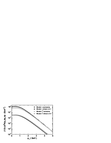
Figure 21: The model predicted transverse momentum distributions of direct $\Sigma^{0}$ and $\Lambda$, inclusive $\Sigma^{0}$, and exclusive $\Lambda$. The decay contribution from $\Sigma^{0}$, $\Xi^{-}$, $\Xi^{0}$ and $\Omega$ to the exclusive $\Lambda$ are removed.

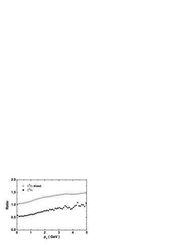
Figure 22: The ratio $\Sigma^{0}/\Lambda$ as a function of transverse momentum, with and without considering decay contribution.

Since it is difficult to extract $\Sigma^{0}$ through electromagnetic decay, $\Sigma^{+}$ may be easier to be determined if $\pi^{0}$ is well measured. Its production is supposed to be similar to $\Sigma^{0}$. The expected $\Sigma^{+}$ production is shown in Fig. 23.

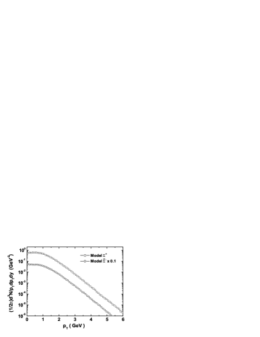
Figure 23: The expected transverse momentum distributions of direct $\Sigma^{+}$and $\bar{\Sigma}^{-}$. No feed-down correction is applied.

$\Lambda(1405)$ $0(\frac{1}{2}^{-})$ and $\Lambda(1520)$ $0(\frac{3}{2}^{-})$ are regarded as singlet states. It is not easy to determine their wave functions in quark-diquark model, and it is hard to distinguish them from the states $(L=1,S=\frac{3}{2})$ and $(L=1,S=\frac{1}{2})$. A rough estimation of $\Lambda(1405)$ and $\Lambda(1520)$ production is shown in Fig. 24, where $\Lambda(1405)$ and $\Lambda(1520)$ are, respectively, supposed to be $(L=1,S=\frac{1}{2})$ octet and $(L=1,S=\frac{3}{2})$ octet. The details on their wave function construction is given in Appendix A.

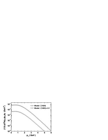
Figure 24: The model calculated transverse momentum distributions of $\Lambda(1405)$ and $\Lambda(1520)$, with the wave functions listed in Appendix A. No feed-down correction is applied.

At the end of the discussion on hadron spectra, we consider the ratio $\bar{\Omega}^{+}/\Omega^{-}$. When diquarks are considered as constituents of the strongly coupled QGP, the strange chemical potential of the system will increase due to the negative strange numbers of diquarks $us$ and $ds$. In our calculations, the strange chemical potential $\mu_{S}=9.35$ MeV is extracted from the strange charge conservation. In this case, the strange quark and diauark $ss$ will carry negative chemical potentials, $\mu_{s}=-0.35$ MeV and $\mu_{ss}=-0.7$ MeV sign:diquark_Omega . The string fragmentation model sign:Omega/OmegaString with diquarks gives similar result. However, the ratio in the calculation without diquarks is $\overline{\Omega}^{+}/\Omega^{-}\leq 1$ sign:coal_3 ; sign:itro_Rafelski_phL .

As shown in Table 3, the ratio $\overline{\Omega}^{+}/\Omega^{-}=1.011$ is consistent with the STAR measurement sign:exp_Ratio_STAR_Omega . While the diquarks are supposed in thermal equilibrium in our model, and the current data are still with large statistical and systematic errors, the qualitative conclusion of $\overline{\Omega}^{+}/\Omega^{-}>1$ is supposed not to be changed.

As pointed above, the thermalization of final state hadrons are omitted in all of the calculations. Considering the interactions which are not inserted in our treatments, some of the dominant hadrons would be partially thermalized effectively. Comparing with the RHIC data, $\pi$, $K$, $p$ and $\Lambda$ may be well thermalized, while the heavy baryons may be not.

V Summary

We have developed a phenomenological model to describe hadron production in relativistic heavy ion collisions. In our model, the QGP evolution and hadron transport are coupled to each other in a self-consistent way. The strongly coupled QGP, including not only gluons and quarks but also their resonant states like diquarks, is described by ideal hydrodynamics, and the hadrons emitted from the QGP satisfy transport equations with loss and gain terms. The hadron decay is effectively reflected in the medium absorption and hadron spectra. Due to the feedback of the hadron emission, the hadronization hypersurface of the parton fluid shrinks with a constant velocity. The splitting of the fluid due to its fast expansion in the later stage and the hadron emission is also effectively considered, by introducing a ratio of the volume of the QGP droplets to the whole volume of the system. We applied our model to calculate the final state hadron spectra in heavy ion collisions. From the comparison with the RHIC data, most of the hadron spectra and hadron ratios can be reasonably described in our model.

The model deserves further improvement in future studies. Unlike quarks and gluons, diquarks in QGP are resonant states and they should behave differently. As a consequence, the assumption that the baryon cross section is $1.5$ times the meson cross section, which arises from the constituent quark model, should be reconsidered carefully. Since mesons are described by transport equations in our model, the assumption of diquark thermalization is in principle not self-consistent. Different types of hadrons will have different thermalization time. Light hadrons are easy but heavy hadrons are difficult to get thermalized. In our current treatment, the relaxation time in hadron transport equations is taken to be infinity, and therefore, no hadron can be thermalized in the whole evolution. The treatment of the QGP fluid splitting is also too simple in our model. When the model is improved, it can be used to calculate more hadron distributions like elliptic flowsign:v2flow01 ; sign:phiflow , which is considered to be sensitive to the thermalization of the parton system in the early stage of heavy ion collisions.
Acknowledgements: We are grateful to Wojciech Broniowski, Huanzhong Huang, Rudolph C. Hwa, Yuxin Liu, Sevil Salur, Qubing Xie, Nu Xu and Weining Zhang for useful discussions. The work is supported in part by the grants No. NSFC10547001 and 10425810.

Appendix A Rewriting the Baryon Wave Functions

The SU(6) baryon wave functions can be rewritten in the quark-diquark model sign:diquark_form ; sign:diquark_Lamda . The $(\frac{1}{2})^{+}$ and $(\frac{3}{2})^{+}$ s-wave intermediate baryon states are introduced as

$$B_{\frac{1}{2},+{1\over 2}}(A,q) = {1\over\sqrt{3}}\left[\sqrt{2}A_{+}q^{\downarrow}-A_{0}q^{\uparrow}\right],$$

$$B_{\frac{1}{2},+{1\over 2}}(S,q) = Sq^{\uparrow},$$

$$B_{\frac{3}{2},+{3\over 2}}(A,q) = A_{+}q^{\uparrow},$$

$$B_{\frac{3}{2},+{1\over 2}}(A,q) = {1\over\sqrt{3}}\left[A_{+}q^{\downarrow}+\sqrt{2}A_{0}q^{\uparrow}\right],$$ (40)

where $S$ and $A$ represent a scalar and an axial-vector diquark state, respectively. The final baryon states can be expressed in terms of certain combinations of these intermediate baryon states sign:diquark_baryon ; sign:diquark_Omega . The wave functions are expressed as

$$|{p}\rangle = \frac{1}{\sqrt{3}}\Big{[}B_{\frac{1}{2}}(A_{uu},d)-\sqrt{\frac{1}{2}}B_{\frac{1}{2}}(A_{ud},u)$$

$$+\sqrt{\frac{3}{2}}B_{\frac{1}{2}}(S_{ud},u)\Big{]},$$

$$|{n}\rangle = \frac{1}{\sqrt{3}}\Big{[}-B_{\frac{1}{2}}(A_{dd},u)+\sqrt{\frac{1}{2}}B_{\frac{1}{2}}(A_{ud},d)$$

$$+\sqrt{\frac{3}{2}}B_{\frac{1}{2}}(S_{ud},d)\Big{]},$$

$$|{\Lambda}\rangle = \frac{1}{\sqrt{3}}\Big{[}\sqrt{\frac{3}{4}}B_{\frac{1}{2}}(A_{us},d)-\sqrt{\frac{3}{4}}B_{\frac{1}{2}}(A_{ds},u)$$

$$+\sqrt{\frac{1}{4}}B_{\frac{1}{2}}(S_{us},d)-\sqrt{\frac{1}{4}}B_{\frac{1}{2}}(S_{ds},u)$$

$$+B_{\frac{1}{2}}(S_{ud},s)\Big{]},$$

$$|{\Sigma^{0}}\rangle = \frac{1}{\sqrt{3}}\Big{[}B_{\frac{1}{2}}(A_{ud},s)-\sqrt{\frac{1}{4}}B_{\frac{1}{2}}(A_{us},d)$$

$$-\sqrt{\frac{1}{4}}B_{\frac{1}{2}}(A_{ds},u)+\sqrt{\frac{3}{4}}B_{\frac{1}{2}}(S_{us},d)$$

$$+\sqrt{\frac{3}{4}}B_{\frac{1}{2}}(S_{ds},u)\Big{]},$$

$$|{\Sigma^{+}}\rangle = -\frac{1}{\sqrt{3}}\Big{[}B_{\frac{1}{2}}(A_{uu},s)-\sqrt{\frac{1}{2}}B_{\frac{1}{2}}(A_{us},u)$$

$$+\sqrt{\frac{3}{2}}B_{\frac{1}{2}}(S_{us},u)\Big{]},$$

$$|{\Sigma^{-}}\rangle = \frac{1}{\sqrt{3}}\Big{[}B_{\frac{1}{2}}(A_{dd},s)-\sqrt{\frac{1}{2}}B_{\frac{1}{2}}(A_{ds},d)$$

$$+\sqrt{\frac{3}{2}}B_{\frac{1}{2}}(S_{ds},d)\Big{]},$$

$$|{\Xi^{0}}\rangle = \frac{1}{\sqrt{3}}\Big{[}-B_{\frac{1}{2}}(A_{ss},u)+\sqrt{\frac{1}{2}}B_{\frac{1}{2}}(A_{us},s)$$

$$+\sqrt{\frac{3}{2}}B_{\frac{1}{2}}(S_{us},s)\Big{]},$$

$$|{\Xi^{-}}\rangle = \frac{1}{\sqrt{3}}\Big{[}-B_{\frac{1}{2}}(A_{ss},d)+\sqrt{\frac{1}{2}}B_{\frac{1}{2}}(A_{ds},s)$$ (41)

$$+\sqrt{\frac{3}{2}}B_{\frac{1}{2}}(S_{ds},s)\Big{]}$$

for the SU(3) octet baryons, and

$$|{\Delta^{++}}\rangle = B_{\frac{3}{2}}(A_{uu},u),$$

$$|{\Delta^{+}}\rangle = \frac{1}{\sqrt{3}}\Big{[}B_{\frac{3}{2}}(A_{uu},d)+\sqrt{2}B_{\frac{3}{2}}(A_{ud},u)\Big{]},$$

$$|{\Delta^{0}}\rangle = \frac{1}{\sqrt{3}}\Big{[}B_{\frac{3}{2}}(A_{dd},u)+\sqrt{2}B_{\frac{3}{2}}(A_{ud},d)\Big{]},$$

$$|{\Delta^{-}}\rangle = B_{\frac{3}{2}}(A_{dd},d),$$

$$|{\Sigma^{*+}}\rangle = \frac{1}{\sqrt{3}}\Big{[}B_{\frac{3}{2}}(A_{uu},s)+\sqrt{2}B_{\frac{3}{2}}(A_{us},u)\Big{]},$$

$$|{\Sigma^{*0}}\rangle = \frac{1}{\sqrt{3}}\Big{[}B_{\frac{3}{2}}(A_{us},d)+B_{\frac{3}{2}}(A_{ds},u)+B_{\frac{3}{2}}(A_{ud},s)\Big{]},$$

$$|{\Sigma^{*-}}\rangle = \frac{1}{\sqrt{3}}\Big{[}B_{\frac{3}{2}}(A_{dd},s)+\sqrt{2}B_{\frac{3}{2}}(A_{ds},d)\Big{]},$$

$$|{\Xi^{*0}}\rangle = \frac{1}{\sqrt{3}}\Big{[}B_{\frac{3}{2}}(A_{ss},u)+\sqrt{2}B_{\frac{3}{2}}(A_{us},s)\Big{]},$$

$$|{\Xi^{*-}}\rangle = \frac{1}{\sqrt{3}}\Big{[}B_{\frac{3}{2}}(A_{ss},d)+\sqrt{2}B_{\frac{3}{2}}(A_{ds},s)\Big{]},$$

$$|{\Omega^{-}}\rangle = B_{\frac{3}{2}}(A_{ss},s)$$ (42)

for the decuplet baryons. From these expressions, we can get the factor $C_{I}$ in Eqs. (27) and (31) to complete the production rate.

There might be other orthogonal baryon states. From the Tables of Particle Physics sign:PDG2006 , $N(1440)$ $\frac{1}{2}(\frac{1}{2}^{+})$ and $N(1710)$ $\frac{1}{2}(\frac{1}{2}^{+})$ are conjectured to be the orthogonal states of $p$ and $n$. Other possible orthogonal states are $\Lambda(1600)$ $0(\frac{1}{2}^{+})$, $\Lambda(1810)$ $0(\frac{1}{2}^{+})$, $\Sigma(1660)$ $1(\frac{1}{2}^{+})$ and $\Sigma(1880)$ $1(\frac{1}{2}^{+})$ of $\Lambda$ and $\Sigma$, $N(1720)$ $\frac{1}{2}(\frac{3}{2}^{+})$ of $\Delta^{+}$ and $\Delta^{0}$, $\Lambda(1890)$ $0(\frac{3}{2}^{+})$ and $\Sigma(1840)$ $1(\frac{3}{2}^{+})$ of $\Sigma^{*}(1385)$, and some unknown orthogonal states of $\Xi$ and $\Xi^{*}(1530)$. There are 24 such particles which belong to two $(\frac{1}{2})^{+}$ octets and a $(\frac{3}{2})^{+}$ octet.

The wave functions of the orthogonal baryon states in $(\frac{3}{2})^{+}$ decuplet can be determined. For example,

$$|{\Lambda}_{2}\rangle^{\{8\}}_{S=\frac{3}{2}} \!\!= \!\!\frac{1}{\sqrt{2}}\left[B_{\frac{3}{2}}(A_{us},d)-B_{\frac{3}{2}}(A_{ds},u)\right],$$ (43)

$$|{\Sigma^{0}_{2}}\rangle^{\{8\}}_{S=\frac{3}{2}} \!\!= \!\!\frac{1}{\sqrt{6}}\left[B_{\frac{3}{2}}(A_{us},d)+B_{\frac{3}{2}}(A_{ds},u)-2B_{\frac{3}{2}}(A_{ud},s)\right].$$

There are two orthogonal baryon states in $(\frac{1}{2})^{+}$ octet. Their wave functions are not unique. Considering that the first octet state is the mixed state of $Aq$ and $Sq$, a most possible assumption is that the second octet state should be the corresponding mixed state, and the third one contains no mixing. Therefore, we have

$$|{N^{+}_{2}}\rangle^{\{8\}}_{S=\frac{1}{2}} \!\!= \!\!\frac{1}{\sqrt{3}}\Big{[}B_{\frac{1}{2}}(A_{uu},d)-\sqrt{\frac{1}{2}}B_{\frac{1}{2}}(A_{ud},u)$$

$$-\sqrt{\frac{3}{2}}B_{\frac{1}{2}}(S_{ud},u)\Big{]},$$

$$|{N^{+}_{3}}\rangle^{\{8\}}_{S=\frac{1}{2}} \!\!= \!\!\frac{1}{\sqrt{3}}\left[B_{\frac{1}{2}}(A_{uu},d)+\sqrt{2}B_{\frac{1}{2}}(A_{ud},u)\right],$$

where, $N_{2}^{+}$ corresponds to $N(1440)^{+}$ and $N_{3}^{+}$ to $N(1710)^{+}$. The other orthogonal baryon wave functions with positive parity are similar.

The wave functions of some of the $(\frac{1}{2})^{-}$ and $(\frac{3}{2})^{-}$ resonances are not clear. It is hard to distinguish a $(\frac{1}{2})^{-}$ or a $(\frac{3}{2})^{-}$ state from the two candidates $(L=1,S=\frac{1}{2})$ and $(L=1,S=\frac{3}{2})$. For simplicity, all $(\frac{1}{2})^{-}$ baryons, except $\Delta$, are regarded as $S=\frac{1}{2}$ octet states and all $(\frac{3}{2})^{-}$ baryons are regarded as $S=\frac{3}{2}$ octet or decuplet states.

$\Lambda(1405)$ $0(\frac{1}{2}^{-})$ and $\Lambda(1520)$ $0(\frac{3}{2}^{-})$ are regarded as singlet states sign:PDG2006 . The quark-diquark wave functions of them are unknown. Approximately, Their wave functions are written as $S=\frac{1}{2}$ octet and $S=\frac{3}{2}$ octet.

Appendix B Effective Lagrangian and Matrix Elements of Production Cross Section

In calculating the hadron production rate, only lowest order interactions are considered. As there are not enough data to determine the coupling modes and constants, we choose only some of the most simple coupling channels. To further reduce the number of parameters, we use two universal coupling constants $g_{M}$ for meson interactions with two quarks and $g_{B}$ for baryon interactions with a quark and a diquark. The meson sector of the effective Lagrangian density is listed in Tab.4 for different meson. The influence of P-wave and D-wave is neglected.

$Meson$	$\quad L_{eff}$	$\qquad\qquad|M_{spin}|^{2}$
${{0}^{-}}$	$ig_{{}_{M}}\bar{q}_{1}\gamma_{5}q_{2}\phi$	$\frac{g_{M}^{2}}{2}\left[m_{M}^{2}-(m_{q1}-m_{q2})^{2}\right]$
${{0}^{+}}$	$ig_{{}_{M}}\bar{q}_{1}q_{2}\phi$	$\frac{g_{M}^{2}}{2}\left[m_{M}^{2}-(m_{q1}+m_{q2})^{2}\right]$
${{1}^{-}}$	$ig_{{}_{M}}\bar{q}_{1}\gamma_{\mu}q_{2}\omega_{\mu}$	$\frac{g_{M}^{2}\left[m_{M}^{2}-(m_{q1}-m_{q2})^{2}\right]}{2}\left[\frac{(m_{q1}+m_{q2})^{2}}{m_{M}^{2}}+2\right]$
${{1}^{+}}$	$ig_{{}_{M}}\bar{q}_{1}\gamma_{\mu}\gamma_{5}q_{2}\omega_{\mu}$	$\frac{g_{M}^{2}\left[m_{M}^{2}-(m_{q1}+m_{q2})^{2}\right]}{2}\left[\frac{(m_{q1}-m_{q2})^{2}}{m_{M}^{2}}+2\right]$
${{2}^{+}}$	$ig_{{}_{M}}\bar{q}_{1}\gamma_{\mu}\gamma_{\nu}q_{2}\kappa_{\mu\nu}$	$\frac{3g_{M}^{2}}{10}\left[m_{M}^{2}-(m_{q1}+m_{q2})^{2}\right]$

Table 4: The effective interactions and the corresponding scattering matrix elements $|M_{spin}|^{2}$ = $|M|^{2}/3$ for different mesons.

For the baryon sector of the effective Lagrangian density, we take

$$L_{qSB} = ig_{B}\;\bar{B}qS,$$ (45)

$$L_{qAB1} = ig_{B}\;\bar{B}\gamma_{\mu}\gamma_{5}qA_{\mu},$$

$$|M|^{2}_{S} \!\!= \!\!{g_{B}^{2}}\left[(m_{B}+m_{q})^{2}-m_{S}^{2}\right],$$

$$|M|^{2}_{A} \!\!= \!\!\frac{g_{B}^{2}}{3}\left[(m_{B}+m_{q})^{2}-m_{A}^{2}\right]\left[\frac{(m_{B}-m_{q})^{2}}{m_{A}^{2}}+2\;\right]$$

for the baryons with $J^{P}=\frac{1}{2}^{+}$, $L=0$ and $S=\frac{1}{2}$. Note that the scattering matrix elements here are equivalent to the expressions in sign:diquark_Omega .

For $J^{P}=\frac{1}{2}^{-}$ sign:Lag_123 , $L=1$ and $S=\frac{1}{2}$, we use

$$L_{qSB} = \frac{ig_{B}}{m_{B}+m_{q}}\;\bar{B}\gamma_{5}\gamma_{\mu}q\partial_{\mu}S,$$ (46)

$$L_{qAB1} = \frac{ig_{B}}{2m_{A}}\;\bar{B}\sigma_{\mu\nu}q\partial_{\nu}A_{\mu},$$

$$|M|^{2}_{S} \!\!= \!\!{g_{B}^{2}}\left[(m_{B}-m_{q})^{2}-m_{S}^{2}\right],$$

$$|M|^{2}_{A} \!\!= \!\!\frac{g_{B}^{2}}{6}\left[(m_{B}-m_{q})^{2}-m_{A}^{2}\right]\left[\frac{(m_{B}+m_{q})^{2}}{m_{A}^{2}}+\frac{1}{2}\;\right]$$

with the definition $\sigma_{\mu\nu}=-i[\gamma_{\mu},\gamma_{\nu}]/2$. The expression of $L_{qSB}$ here gives the same result as the direct coupling sign:Lag1p2min . For $J^{P}=\frac{1}{2}^{-}$, $L=1$ and $S=\frac{3}{2}$, the scattering matrix elements are supposed to be the same.

We choose

$$L_{qAB} = ig_{B}\;\bar{B}_{\mu}\gamma_{5}qA_{\mu},$$

$$|M|^{2}_{A} = \frac{g_{B}^{2}}{18}\left[(m_{B}-m_{q})^{2}-m_{A}^{2}\;\right]$$ (47)

$$\times\left[\frac{(m_{B}^{2}+m_{A}^{2}-m_{q}^{2})^{2}}{m_{B}^{2}m_{A}^{2}}+8\;\right]$$

for $J^{P}=\frac{3}{2}^{+}$ sign:Lag_RS , $L=0$ and $S=\frac{3}{2}$, and

$$L_{qSB} = \frac{ig_{B}}{m_{S}}\;\bar{B}_{\mu}\gamma_{5}q\partial_{\mu}S,$$

$$|M|^{2}_{S} = \frac{g_{B}^{2}}{6}\left[(m_{B}-m_{q})^{2}-m_{S}^{2}\right]$$ (48)

$$\times\left[\frac{(m_{B}^{2}+m_{S}^{2}-m_{q}^{2})^{2}}{m_{B}^{2}m_{S}^{2}}-4\;\right]$$

for $J^{P}=\frac{3}{2}^{-}$, $L=1$ and $S=\frac{1}{2}$. For the axial-vector couplings, the matrix element is replaced by

$$|M|^{2}_{A} = \frac{g_{B}^{2}}{18}\left[(m_{B}+m_{q})^{2}-m_{A}^{2}\;\right]$$ (49)

$$\times\left[\frac{(m_{B}^{2}+m_{A}^{2}-m_{q}^{2})^{2}}{m_{B}^{2}m_{A}^{2}}+8\;\right],$$

and the expression for $J^{P}=\frac{3}{2}^{-}$, $L=1$ and $S=\frac{3}{2}$ is the same.

We employ

$$L_{qAB} = \frac{ig_{B}}{m_{A}}\;\bar{B}_{\mu\nu}q\partial_{\mu}A_{\nu},$$

$$M|^{2}_{A} = \frac{g_{B}^{2}}{48}\left[(m_{B}+m_{q})^{2}-m_{A}^{2}\right]$$ (50)

$$\times\left[\frac{(m_{B}^{2}+m_{A}^{2}-m_{q}^{2})^{2}}{m_{B}^{2}m_{A}^{2}}-4\right]$$

$$\times\left[\frac{(m_{B}^{2}+m_{A}^{2}-m_{q}^{2})^{2}}{m_{B}^{2}m_{A}^{2}}+5.6\right]$$

for $J^{P}=\frac{5}{2}^{-}$, $L=1$ and $S=\frac{3}{2}$, where the expression of the spin-$\frac{5}{2}$ projector can be found in sign:Lag_25 , and

$$L_{qSB} = \frac{ig_{B}}{m_{S}^{2}}\;\bar{B}_{\mu\nu}q\partial_{\mu}\partial_{\nu}S,$$

$$|M|^{2}_{S} = \frac{g_{B}^{2}}{16}\left[(m_{B}+m_{q})^{2}-m_{S}^{2}\right]$$ (51)

$$\times\left[\frac{(m_{B}^{2}+m_{S}^{2}-m_{q}^{2})^{2}}{m_{B}^{2}m_{S}^{2}}-4\;\right]^{2}$$

for $J^{P}=\frac{5}{2}^{+}$, $L=2$ and $S=\frac{1}{2}$.

References

- (1) U. W. Heinz, Nucl. Phys. A685, 414(2001).
- (2) J. Stachel, Nucl. Phys. A654, 119c(1999).
- (3) J. Rafelski and J. Letessier, Phys. Lett. B469, 12(1999).
- (4) P. Huovinen, Nucl. Phys. A761, 296(2005).
- (5) G. E. Brown and M. Rho, Phys. Rev. Lett. 66, 2720(1991); G. E. Brown et al., nucl-th/0608023.
- (6) P. F. Kolb and U. W. Heinz, nucl-th/0305084.
- (7) W. Florkowski, W. Broniowski and A. Baran, J. Phys. G31, S1087(2005).
- (8) C. Nonaka and S. A. Bass, nucl-th/0607018.
- (9) T. S. Bir and J. Zimanyi, Phys. Lett. B113, 6(1982); Nucl. Phys. A395, 525(1983).
- (10) T. S. Bir, P. Lvai and J. Zimanyi, J. Phys. G28, 1561(2002).
- (11) R. J. Fries, J. Phys. G30, S853(2004).
- (12) R. J. Fries, B. Mller, C. Nonaka and S. A. Bass, Phys. Rev. Lett. 90, 202303 (2003); R. J. Fries, B. Mller, C. Nonaka and S. A. Bass, Phys. Rev. C68, 044902 (2003).
- (13) V. Greco, C. M. Ko, and P. Lvai, Phys. Rev. Lett. 90, 202302 (2003); V. Greco, C. M. Ko, and P. Lvai, Phys. Rev. C68, 034904 (2003).
- (14) R. C. Hwa and C. B. Yang, nucl-th/0602024.
- (15) M. Gyulassy, P. Levai and I. Vitev, Phys. Rev. Lett. 85, 5535(2000); M. Gyulassy, P. Levai and I. Vitev, Nucl. Phys. B594, 371(2001).
- (16) Q. Wang and X. N. Wang, Phys. Rev. C71, 014903 (2005).
- (17) L. G. Moretto et al., Phys. Rev. Lett. 94, 202701(2005).
- (18) J. Adams et al., the STAR Collaboration, Phys. Rev. C71, 044906(2005).
- (19) P. F. Kolb and R. Rapp, Phys. Rev. C67, 044903(2003).
- (20) J. Rafelski and J. Letessier, Eur. Phys. J. A29, 107(2006).
- (21) H. Stocker et al., Phys. Lett. B95, 192(1980).
- (22) G. Bertsch et al., Phys. Rev. D37, 1202(1988).
- (23) W. H. Barz, B. L. Friman, J. Knoll and H. Schulz, Phys. Lett. B242, 328(1990).
- (24) I. Arsene et al., Nucl. Phys. A757, 1(2005); B. B. Back et al., Nucl. Phys. A757, 28(2005); J. Adams et al., Nucl. Phys. A757, 102(2005); K. Adcox et al., Nucl. Phys. A757, 184 (2005).
- (25) D. Teaney, J. Lauret and E. V. Shuryak, Phys. Rev. Lett. 86, 4783(2001); P. F. Kolb, P. Huovinen, U. Heinz and H. Heiselberg, Phys. Lett. B500, 232(2001).
- (26) H. Miao, Z. B. Ma and C. S. Gao, J. Phys. G29, 2187(2003).
- (27) E. V. Shuryak and I. Zahed, Phys. Rev. D70, 054507(2004).
- (28) M. Huang, P. F. Zhuang and W. Q. Chao, Phys. Rev. D67, 065015(2003).
- (29) S. K. Karn, hep-ph/0510239.
- (30) S. Calogero, J. Math. Phys. 45, 4042(2004).
- (31) L. Yan, P. F. Zhuang and N. Xu, Phys. Rev. Lett. 97, 232301(2006).
- (32) J. W. Clark, J. Cleymans and J. Rafelski, Phys. Rev. C33, 703(1986).
- (33) H. Miao, C. S. Gao and P. F. Zhuang, Commun. Theor. Phys. 46, 1040(2006).
- (34) C. S. Gao, in JingShin Theoretical Physics Symposium in Honor of Professor Ta-You Wu, edited by J. P. Hsu and L. Hsu, (World Scientific, 1998) 362.
- (35) H. Miao and C. S. Gao, J. Phys. G31, 179(2005).
- (36) W. M. Yao et al., (Particle Data Group), J. Phys. G33, 1(2006).
- (37) Z. Fodor and S. Katz, JHEP 0203, 014(2002).
- (38) F. Karsch, Nucl. Phys. B(Proc. Suppl.) 83-84, 14(2000).
- (39) D. B. Lichtenberg, W. Namgung, J. G. Wills and E. Predazzi, Z. Phys. C19, 19 (1983); D. B. Lichtenberg, R. Roncaglia and E. Predazzi, hep-ph/9611428.
- (40) J. P. Boris, D. L. Book, J. Comp. Phys. 11, 38(1973); J. P. Boris, D. L. Book, and K. Hain, J. Comp. Phys. 18, 248(1995).
- (41) D. H. Rischke, S. Bernard, and J. A. Maruhn, Nucl. Phys. A595, 346(1995); D. H. Rischke, Y. Prs, and J. A. Maruhn, Nucl. Phys. A595, 383 (1995).
- (42) H. Miao, Z. B. Ma and C. S. Gao, Commun. Theor. Phys. 38, 698(2002).
- (43) J. D. Bjorken, Phys. Rev. D27, 140(1983).
- (44) A. Bialas, M. Bleszynski and W. Czyz, Nucl. Phys. B111, 461(1976).
- (45) S. S. Adler et al, the PHENIX Collaboration, Phys. Rev. C69, 034909 (2004).
- (46) B. B. Back et al., the PHOBOS Collaboration, Phys. Rev. C70, 051901(R) (2004).
- (47) B. I. Abelev et al., the STAR Collaboration, Phys. Rev. Lett. 97, 152301(2006).
- (48) M. Estienne (for the STAR Collaboration), J. Phys. G31, S873(2005).
- (49) J. Adams et al., the STAR Collaboration, Nucl. Phys. A757, 102(2005); J. Adams et al., the STAR Collaboration, Phys. Rev. Lett. 98, 062301(2007).
- (50) J. Adams et al., the STAR Collaboration, nucl-ex/0601042.
- (51) J. Adams et al., the STAR Collaboration, Phys. Rev. C71, 064902(2005).
- (52) J. Adams et al., the STAR Collaboration, Phys. Lett. B612, 181(2005).
- (53) S. S. Adler et al, the PHENIX Collaboration, Phys. Rev. C72, 014903(2005).
- (54) J. Adams et al., the STAR Collaboration, Phys. Rev. Lett. 97, 132301 (2006); S. Salur, Ph.D. thesis, Yale University, 2006.
- (55) R. Witt (for the STAR Collaboration), nucl-ex/0701063.
- (56) S-L. Blyth (for the STAR Collaboration), nucl-ex/0608019.
- (57) S. Salur (for the STAR Collaboration), nucl-ex/0606006.
- (58) J. Harris, Overview of First Results from Star, (for STAR Collaboration), Quark Matter 2002.
- (59) C. Adler et al., the STAR Collaboration, Phys. Rev. Lett. 89, 092301(2002).
- (60) K. Adcox et al., the PHENIX Collaboration, Phys. Rev. Lett. 89, 092302(2002).
- (61) M. Bleicher et al., Phys. Rev. Lett. 88, 202501(2002).
- (62) J. Zimanyi et al., hep-ph/0103156.
- (63) S.S. Adler et al., the PHENIX Collaboration, Phys. Rev. Lett. 91, 182301(2003); J. Adams et al., the STAR Collaboration, Phys. Rev. Lett. 95, 122301 (2005).
- (64) J. H. Chen et al, Phys. Rev. C74, 064902(2006).
- (65) M. I. Pavkovi, Phys. Rev. D13, 2128(1976).
- (66) B. Q. Ma, I. Schmidt and J. J. Yang, Phys. Lett. B477, 107(2000).
- (67) G. Penner and U. Mosel, Phys. Rev. C66, 055211(2002).
- (68) S. L. Zhu, W-Y. P. Hwang and Y. B. Dai, Phys. Rev. C59, 442(1999).
- (69) W. Rarita and J. Schwinger, Phys. Rev. 60, 61(1941).
- (70) V. Shklyar, G. Penner and U. Mosel, hep-ph/0301152.