First Order Relativistic Three-Body Scattering

Abstract

Relativistic Faddeev equations for three-body scattering at arbitrary energies are formulated in momentum space and in first order in the two-body transition-operator directly solved in terms of momentum vectors without employing a partial wave decomposition. Relativistic invariance is incorporated within the framework of Poincaré invariant quantum mechanics, and presented in some detail. Based on a Malfliet-Tjon type interaction, observables for elastic and break-up scattering are calculated up to projectile energies of 1 GeV. The influence of kinematic and dynamic relativistic effects on those observables is systematically studied. Approximations to the two-body interaction embedded in the three-particle space are compared to the exact treatment.

I Introduction

Light nuclei can be accurately modeled as systems of nucleons interacting via effective two and three-body forces motivated e.g. by meson exchange. This picture is expected to break down at a higher energy scale where the physics is more efficiently described in terms of sub-nuclear degrees of freedom. One important question in nuclear physics is to understand the limitations of models of nuclei as systems of interacting nucleons. Few-body methods have been an essential tool for determining model Hamiltonians that describe low-energy nuclear physics. Few-body methods also provide a potentially useful framework for testing the limitations of models of nuclei as few nucleon systems, however this requires extending the few-body models and calculations to higher energy scales. There are a number of challenges that must be overcome to extend these calculations to higher energies. These include replacing the non-relativistic theory by a relativistic theory, limitations imposed by interactions fit to elastic scattering data, new degrees of freedom that appear above the pion production threshold, as well as numerical problems related to the proliferation of partial wave at high energies. In this paper we address some of these questions. We demonstrate that it is possible to now perform relativistic three-body scattering calculations at energies up to 1 GeV laboratory kinetic energy. The key elements of our success is the use of direct integration methods that avoid the use of partial waves and new techniques for treating functions of non-commuting operators that appear in the relativistic nucleon-nucleon interactions.

During the last two decades calculations of nucleon-deuteron scattering based on momentum-space Faddeev equations faddeev experienced large improvements and refinements. It is fair to state that below about 200 MeV projectile energy the momentum-space Faddeev equations for three-nucleon (3N) scattering can now be solved with high accuracy for realistic two- and three-nucleon interactions. A summary of these achievements can be found in Refs. wgphysrep ; wgarticle ; kuros ; sauer . The approach described there is based on using angular momentum eigenstates for the two- and three-body systems. This partial wave decomposition replaces the continuous angle variables by discrete orbital angular momentum quantum numbers, and thus reduces the number of continuous variables to be discretized in a numerical treatment. For low projectile energies the procedure of considering orbital angular momentum components appears physically justified due to arguments related to the centrifugal barrier and the short range of the nuclear force. If one considers three-nucleon scattering at a few hundred MeV projectile kinetic energy, the number of partial waves needed to achieve convergence proliferates, and limitations with respect to computational feasibility and accuracy are reached. It appears therefore natural to avoid a partial wave representation completely and work directly with vector variables. This is common practice in bound state calculations of few-nucleon systems based on variational Arriaga95a and Green’s function Monte Carlo (GFMC) methods Carlson87a ; Carlson88a ; Zabolitzki82a ; Carlson99a and was for the first time applied in momentum space Faddeev calculations for bound states in bound3d and for scattering at intermediate energies in Ref. scatter3d .

The key advantage of a formulation of the Faddeev equations in terms of vector variables lies in its applicability at higher energies, where special relativity is expected to become relevant. Poincaré invariance is an exact symmetry that should be satisfied by all calculations, however in practice consistent relativistic calculations are more numerically intensive, thus making their nonrelativistic counterpart a preferred choice. Furthermore, estimates of relativistic effects have been quantitatively small for 3N scattering below 200 MeV witalar1 ; witalar2 ; witalar3 with the exception of some breakup cross sections in certain phase space regions Skibin , indicating that at those energies non-relativistic calculations have sufficient precision. This is in part because in either a relativistic or non-relativistic model the interactions are designed to fit the same invariant differential cross section moller , which can be evaluated in any frame using standard kinematic Lorentz transformations, so model calculations are designed so that there are no “relativistic corrections” at the two-body level. Three-body interactions can even be chosen so the non-relativistic calculations fit both the two- and three-body invariant cross sections. This can be done in one frame and the invariance of the cross section fixes it in all other frames using standard relativistic kinematics. This, procedure has internal inconsistencies which show up if these models are used as input in larger systems, but they clearly indicate that the problem of identifying relativistic effects is more subtle than simply computing non-relativistic limits. In this paper we focus on differences between relativistic and non-relativistic calculations with two-body input that have the same cross section and use the same two-body wave functions KG ; cps ; keipo .

There are two primary approaches for modeling relativistic few-body problems. One treats Poincaré invariance as a symmetry of a quantum theory, the other is based on quasipotential reductions Frohlich:1983 of formal relations Dyson:1949 ; Schwinger:1951 between covariant amplitudes. One specific realization of this approach is the covariant spectator approach of Ref. stadler . In this paper the relativistic three-body problem is formulated within the framework of Poincaré invariant quantum mechanics. It has the advantage that the framework is valid for any number of particles and the dynamical equations have the same number of variables as the corresponding non-relativistic equations. Poincaré invariance is an exact symmetry that is realized by a unitary representation of the Poincaré group on a three-particle Hilbert space. The dynamics is generated by a Hamiltonian. This feature is shared with the Galilean invariant formulation of non-relativistic quantum mechanics. The Hamiltonian of the corresponding relativistic model differs in how the two-body interactions are embedded in the three-body center of momentum Hamiltonian (mass operator). The equations we use to describe the relativistic few-problem have the same operator form as the nonrelativistic ones, however the ingredients are different.

In this article we want to concentrate on the leading order term of the Faddeev multiple scattering series within the framework of Poincaré invariant quantum mechanics. The first order term contains already most relativistic ingredients which, together with the relativistic free three-body resolvent, gives the kernel of the integral equation. We want to understand essential differences between a relativistic and nonrelativistic approach already on the basis of the first order term. As simplification we consider three-body scattering with spin-independent interactions. This is mathematically equivalent to three-boson scattering. The interactions employed are of Yukawa type, and no separable expansions are employed. In order to obtain a valid estimate of the size of relativistic effects, it is important that the interactions employed in the nonrelativistic and relativistic calculations are phase-shift equivalent. To achieve this we employ here the approach suggested by Kamada-Glöckle KG , which uses a unitary rescaling of the momentum variables to change the nonrelativistic kinetic energy into the relativistic kinetic energy.

This article is organized as follows. Section II discusses the formulation of Poincaré invariant quantum mechanics, and section III discusses the structure of the dynamical two- and three-body mass operators. Scattering theory formulated in terms of mass operators is discussed in section IV. The formulation of the Faddeev equations and techniques for computing the Faddeev kernel are discussed in section V. Details on kinematical aspects of how to construct the cross sections is given in section VI. In Sections VIII and IX we present calculations for elastic and breakup processes in the intermediate energy regime from 0.2 to 1 GeV. Our focus here is to compare different approximations to the embedded interaction with respect to the exact calculation. Our conclusions are in Section X. Two Appendices are devoted to relating the transition matrix elements based on mass operators to the invariant amplitudes with the conventions used in the particle data book and expressing the invariant cross section and differential cross sections worked out directly in laboratory-frame variables.

II Poincaré Invariant Quantum Mechanics

Symmetry under change of inertial coordinate system is the fundamental symmetry of Poincaré invariant quantum mechanics. In special relativity different inertial coordinate systems are related by the subgroup of Poincaré transformations continuously connected to the identity. In this paper the Poincaré group refers to this subgroup, which excludes the discrete transformations of space reflection and time reversal. Wigner wigner proved that a necessary and sufficient condition for quantum probabilities to be invariant under change of inertial coordinate system is the existence of a unitary representation, ${\cal U}(\Lambda,a)$, of the Poincaré group on the model Hilbert space. Equivalent vectors, $|\psi\rangle$ and $|\psi^{\prime}\rangle$, in different inertial coordinate systems are related by:

$$|\psi^{\prime}\rangle={\cal U}(\Lambda,a)|\psi\rangle.$$ (1)

In Poincaré invariant quantum mechanics the dynamics is generated by the time evolution subgroup of ${\cal U}(\Lambda,a)$. The fundamental dynamical problem is to decompose ${\cal U}(\Lambda,a)$ into a direct integral of irreducible representations. This is the analog of diagonalizing the Hamiltonian or time-evolution operator in non-relativistic quantum mechanics. The problem of formulating the dynamics is to construct the dynamical representation ${\cal U}(\Lambda,a)$ of the Poincaré group by introducing realistic interactions in the tensor products of single particle irreducible representations in a manner that preserves the group representation property and essential aspects of cluster separability. The solution to this non-linear problem is achieved by adding suitable interactions to the Casimir operators of non-interacting irreducible representations of the Poincaré group.

Since irreducible representations of the Poincaré group play a central role in both the formulation and solution of the dynamical model, we give a brief summary of the construction of the irreducible representations that we use in this paper. The Poincaré group is a ten parameter group that is the semidirect product of the Lorentz group and the group of spacetime translations. Spacetime translations are generated by the four momentum operator, $P^{\mu}$, and Lorentz transformations are generated by the antisymmetric angular momentum tensor, $J^{\mu\nu}$.

The Pauli Lubanski vector is the four vector operator defined by

$$W^{\mu}=-{1\over 2}\epsilon^{\mu\alpha\beta\gamma}P_{\alpha}J_{\beta\gamma}.$$ (2)

The Casimir operators for the Poincaré group are

$$M^{2}=-\eta_{\mu\nu}P^{\mu}P^{\nu}=H^{2}-\mathbf{P}\cdot\mathbf{P}$$ (3)

and

$$W^{2}=-\eta_{\mu\nu}W^{\mu}W^{\nu}=M^{2}j^{2}$$ (4)

where $\eta_{\mu\nu}$ is the Minkowski metric, $M$ is the mass operator, $H$ is the Hamiltonian, $\mathbf{P}$ is the linear momentum, and $j^{2}$ is the spin.

Positive-mass positive-energy irreducible representations are labeled by eigenvalues of the mass $M$ and spin $j^{2}$. Vectors in an irreducible subspace are square integrable functions of the eigenvalues of a complete set of commuting Hermitian operator-valued functions of the generators $P^{\mu}$ and $J^{\mu\nu}$. In addition to the two invariant Casimir operators, it is possible to find four additional commuting Hermitian functions of the generators. For each of these four commuting observables it is possible to find conjugate operators. These conjugate operators, along with the eigenvalues of the Casimir operators, fix the eigenvalue spectrum of the four commuting Hermitian operators. The irreducible representation space is the space of square integrable functions of the eigenvalues of the four commuting operators. The generators can be expressed as functions of these four operators, their conjugates, and the Casimir invariants fcwp ; bkwp ; wp2 .

In this paper we choose the four commuting operators to be the three components of the linear momentum and the $z$ component of the canonical spin operator. In this representation the four conjugate operators are taken as the partial derivatives of the momentum holding the canonical spin constant (Newton-Wigner position nw operator) and the $x$ component of the canonical spin. While $j_{x}$ is not exactly conjugate to $j_{z}$, the two operators generate the full $SU(2)$ spin algebra. The corresponding eigenstates have the form

$$|\mathbf{p},\mu\rangle:=|(m,j)\mathbf{p},\mu\rangle.$$ (5)

The mass $m$ spin $j$ irreducible representation of the Poincaré group in this basis is determined from the group representation property and the action of rotations, spacetime translations and canonical boosts on the zero momentum eigenstates:

$${\cal U}(R,0)|\mathbf{0},\mu\rangle=|\mathbf{0},\mu^{\prime}\rangle D^{j}_{\mu^{\prime}\mu}(R)$$ (6)

$${\cal U}(I,a)|\mathbf{0},\mu\rangle=e^{-ia^{0}m}|\mathbf{0},\mu\rangle$$ (7)

$${\cal U}(B(p_{m}),0)|\mathbf{0},\mu\rangle=|\mathbf{p},\mu\rangle\sqrt{{E_{p_{m}}\over m}}$$ (8)

where in these equations $R$ is a rotation, $D^{j}_{\mu^{\prime}\mu}(R)$ is the standard $2j+1$ dimensional unitary representation of $SU(2)$, $a=(a^{0},\mathbf{a})$ is a displacement four vector, $B(p_{m})$ is the rotationless Lorentz boost (canonical boost) that transforms $(m,\mathbf{0})$ to $p_{m}:=(E_{p_{m}},\mathbf{p})$,

$$(B(p_{m}))^{\mu}{}_{\nu}:=\left(\begin{array}[]{cc}{E_{p_{m}}/m}&{\mathbf{p}/m}\\ {\mathbf{p}/m}&I+{\mathbf{p}\otimes\mathbf{p}\over m(m+E_{p_{m}})}\end{array}\right),$$ (9)

and $E_{p_{m}}=\sqrt{m^{2}+\mathbf{p}^{2}}$. That the magnetic quantum number remains invariant in (8) under the rotationless boost (9) is the defining property of the canonical spin.

The multiplicative factor on the right side of (8) is fixed up to a phase by unitarity and the normalization convention

$$\langle\mathbf{p}\,^{\prime},\mu^{\prime}|\mathbf{p},\mu\rangle=\delta(\mathbf{p}\,^{\prime}-\mathbf{p})\delta_{\mu^{\prime}\mu}.$$ (10)

With these choices the action of an arbitrary Poincaré transformation on these states is given by

$${\cal U}_{mj}(\Lambda,a)|\mathbf{p},\mu\rangle=|\mathbf{p}\,^{\prime},\mu^{\prime}\rangle\sqrt{E_{p_{m}}^{\prime}\over E_{p_{m}}}D^{j}_{\mu^{\prime}\mu}\left(R_{w}(\Lambda,p_{m})\right)e^{ip_{m}^{\prime}\cdot a},$$ (11)

where $R_{w}(\Lambda,p_{m})$ is the (standard) Wigner rotation,

$$R_{w}(\Lambda,p_{m}):=B^{-1}(\Lambda p_{m})\Lambda B(p_{m}),$$ (12)

and $p_{m}^{\prime}=\Lambda p_{m}$. Since each of the elementary transformations (6,7,8) are unitary, it follows that (11) is unitary. Since every basis vector can be generated from the $\mu=j$ and $\mathbf{P}=\mathbf{0}$ basis vector using equations (6,7,8), representation (11) is also irreducible.

The mass $m$ spin $j$ irreducible representations that are used in this paper have the form (11). The mass $m$ spin $j$ irreducible representation space with basis (5) is denoted by ${\cal H}_{mj}$.

The Hilbert space for the-three nucleon problem is the tensor product of three one-nucelon irreducible representation spaces:

$${\cal H}={\cal H}_{m{1\over 2}}\otimes{\cal H}_{m{1\over 2}}\otimes{\cal H}_{m{1\over 2}}.$$ (13)

In this paper all nucleons are assumed to have the same mass, $m$.

The non-interacting unitary representation of the Poincaré group on ${\cal H}$ is the tensor product of three one-nucleon irreducible representations:

$${\cal U}_{0}(\Lambda,a)={\cal U}_{m{1\over 2}}(\Lambda,a)\otimes{\cal U}_{m{1\over 2}}(\Lambda,a)\otimes{\cal U}_{m{1\over 2}}(\Lambda,a).$$ (14)

As in the case of rotations, the tensor product of irreducible representations of the Poincaré group is reducible. The tensor product of three irreducible representations can be decomposed into a direct integral of irreducible representation using Clebsch-Gordan coefficients for the Poincaré group. The Clebsch-Gordan coefficients for the Poincaré group are known stora ; fch ; bkwp . As in the case of rotations, the Poincaré Clebsch-Gordan coefficients are basis dependent and the three-body irreducible representations can be generated by pairwise coupling. The Poincaré Clebsch-Gordan coefficients can be computed by using $SU(2)$ Clebsch-Gordan coefficients to decompose three-body zero momentum eigenstates states into irreducible $SU(2)$ representations. Three-body irreducible basis vectors are generated by applying Eqs. (6,7,8) to the zero-momentum $SU(2)$ irreducible representations.

The resulting irreducible three-body basis depends on the order of the coupling. In the basis of eigenstates of the three-body linear momentum and canonical spin the irreducible eigenstates are labeled by eigenvalues ${\sf W}$ of the three-body invariant mass, $M_{0}$, the three-body canonical spin, $j$ (for simplicity of notation we use the same label $j$ for the total canonical spin of the three-body system and the single particle canonical spin), the total three-body momentum, $\mathbf{P}$, the $z$ component of the three-body canonical spin, $\mu$, and invariant degeneracy quantum numbers, $d$, that distinguish multiple copies of the same irreducible representation:

$$|({\sf W},j),\mathbf{P},\mu,d\rangle.$$ (15)

For two-particle systems the degeneracy quantum numbers $d$ are discrete (for example they may be taken to be invariant spin and orbital angular momentum quantum numbers) while for more than two particles the degeneracy quantum numbers will normally include invariant sub-energies, which have a continuous eigenvalue spectrum. In addition to the appearance of the degeneracy quantum numbers, the eigenvalue spectrum of the free invariant mass operator, $M_{0}$, is continuous.

These states transform as mass ${\sf W}$ spin $j$ irreducible representations of the Poincaré group under ${\cal U}_{0}(\Lambda,a)$:

$${\cal U}_{0}(\Lambda,a)|({\sf W},j),\mathbf{P},\mu,d\rangle=|({\sf W},j),\mathbf{P}\,^{\prime},\mu^{\prime},d\rangle\sqrt{E_{P_{\sf W}}^{\prime}\over E_{P_{\sf W}}}D^{j}_{\mu^{\prime}\mu}\left(R_{w}(\Lambda,P_{\sf W})\right)e^{iP_{\sf W}^{\prime}\cdot a},$$ (16)

where

$$P^{\prime}_{\sf W}=\Lambda P_{\sf W}\qquad P_{\sf W}:=(\sqrt{{\sf W}^{2}+\mathbf{P}^{2}},\mathbf{P})=(E_{P_{\sf W}},\mathbf{P}).$$ (17)

The quantities ${\sf W},j,d$ are invariants of the representation (16) of ${\cal U}_{0}(\Lambda,a)$.

Because the Poincaré group allows time evolution to be expressed in terms of spatial translations and Lorentz boosts, when particles interact, consistency of the initial value problem requires that the unitary representation of the Poincaré group depends non-trivially on the interactions. The construction of ${\cal U}(\Lambda,a)$ for dynamical models is motivated by the example of Galilean invariant quantum mechanics. The non-relativistic three-body Hamiltonian has the form

$$H={\mathbf{P}^{2}\over 2M_{g}}+h$$ (18)

where the Casimir Hamiltonian, $h$, is the Galilean invariant part of the Hamiltonian and $M_{g}$ is the Galilean mass. In the non-relativistic case interactions are added to the non-interacting Casimir Hamiltonian $h_{0}$ :

$$h=h_{0}+V_{nr}$$ (19)

where the Galilean invariance of $h$ requires that the interaction $V_{nr}$ is rotationally invariant and commutes with and is independent of the linear momentum $\mathbf{P}$. This means that in the corresponding non-relativistic basis

$$\langle{\sf h},\mathbf{P},j,\mu,d|V_{nr}|{\sf h}^{\prime},\mathbf{P}\,^{\prime},j^{\prime},\mu^{\prime},d^{\prime}\rangle=\delta(\mathbf{P}-\mathbf{P}\,^{\prime})\delta_{jj^{\prime}}\delta_{\mu\mu^{\prime}}\langle{\sf h},d\|V^{j}_{nr}\|{\sf h}^{\prime},d^{\prime}\rangle.$$ (20)

where ${\sf h}$ is an eigenvalue of $h_{0}$.

In the Poincaré invariant case Eq. (18) is replaced by

$$H=\sqrt{\mathbf{P}^{2}+M^{2}}$$ (21)

where $M$ in Eq. (21) plays the same role as the Casimir Hamiltonian $h$ in Eq. (18). The corresponding free relativistic Hamiltonian is $H_{0}=\sqrt{\mathbf{P}^{2}+M^{2}_{0}}$. In what follows $\lambda$ denotes the eigenvalue of $M$ to distinguish it from the eigenvalue ${\sf W}$ of $M_{0}$.

A Poincaré invariant dynamics can be constructed by adding an interaction to the non-interacting $M_{0}$ that commutes with and is independent of $\mathbf{P}$ and $j_{z}$:

$$M=M_{0}+V_{r}.$$ (22)

In the non-interacting irreducible basis (15) these conditions require interactions of the form

$$\langle({\sf W},j),\mathbf{P},\mu,d|V_{r}|({\sf W}^{\prime},j^{\prime}),\mathbf{P}\,^{\prime},\mu^{\prime},d^{\prime}\rangle=\delta(\mathbf{P}-\mathbf{P}\,^{\prime})\delta_{jj^{\prime}}\delta_{\mu\mu^{\prime}}\langle{\sf W},d\|V^{j}_{r}\|{\sf W}^{\prime},d^{\prime}\rangle.$$ (23)

The dynamical problem is to find simultaneous eigenstates of the commuting operators $M$, $\mathbf{P}$, $j_{z}$, and $j^{2}$. This is done by diagonalizing $M$ in the irreducible basis (15). The eigenfunctions of $M$ have the form

$$\langle({\sf W},j),\mathbf{P},\mu,d|(\lambda,j^{\prime}),\mathbf{P}\,^{\prime},\mu^{\prime}\rangle=\delta(\mathbf{P}-\mathbf{P}\,^{\prime})\delta_{jj^{\prime}}\delta_{\mu\mu^{\prime}}\langle{\sf W},d,j|\lambda,j\rangle$$ (24)

where the eigenfunctions $\langle{\sf W},d,j|\lambda,j\rangle$ are solutions of

$${\sf W}\langle{\sf W},j,d|\lambda,j\rangle+\sum^{\prime}\int^{\prime}\langle{\sf W},d\|V^{j}_{r}\|{\sf W}^{\prime},d^{\prime}\rangle d{\sf W}^{\prime}dd^{\prime}\langle{\sf W}^{\prime},j,d^{\prime}|\lambda,j\rangle=\lambda\langle{\sf W},j,d|\lambda,j\rangle,$$ (25)

with mass eigenvalue $\lambda$. For two-particle systems the degeneracy quantum numbers $d$ are discrete (for example they may taken to be invariant spin and orbital angular momentum quantum numbers) while for more than two particles the degeneracy quantum numbers will normally include invariant sub-energies, which have a continuous eigenvalue spectrum.

Because $\{M_{0},j^{2},j_{z},\mathbf{P},j_{x},-i\mbox{\boldmath$\nabla$}_{P}\}$ have the same commutations relations as $\{M,j^{2},j_{z},\mathbf{P},j_{x},-i\mbox{\boldmath$\nabla$}_{P}\}$, if the dynamical Poincaré generators are defined as the same functions of these operators wp2 ; bkwp with $M_{0}$ replaced by $M$, it follows that the simultaneous eigenstates

$$|(\lambda,j),\mathbf{P},\mu\rangle$$ (26)

of $M,j^{2},\mathbf{P},j_{z}$ transform as a mass $\lambda$ spin $j$ irreducible representation of the Poincaré group.

Since these eigenstates are complete, this defines the dynamical representation of the Poincaré group on a basis by

$${\cal U}(\Lambda,a)|(\lambda,j),\mathbf{P},\mu\rangle=|(\lambda,j),\mathbf{P}\,^{\prime},\mu^{\prime}\rangle\sqrt{E_{P_{\lambda}}^{\prime}\over E_{P_{\lambda}}}D^{j}_{\mu^{\prime}\mu}\left(R_{w}(\Lambda,P_{\lambda})\right)e^{iP^{\prime}_{\lambda}\cdot a},$$ (27)

where

$$E_{P_{\lambda}}=\sqrt{\lambda^{2}+{\mathbf{P}}^{2}},\qquad P_{\lambda}:=(E_{P},{\mathbf{P}}),\qquad P^{\prime}_{\lambda}=\Lambda P_{\lambda}.$$ (28)

This shows that the solution to the eigenvalue problem (25) provides the desired decomposition of the dynamical unitary representation of the Poincaré group into a direct integral of irreducible representations.

The appearance of the mass eigenvalue $\lambda$ on the right side of Eq. (27) indicates the interaction dependence of this representation. It can happen, for a given choice of irreducible basis, that the coefficient on the right hand side of (27) is independent of the mass eigenvalue for a subgroup of the Poincaré group. For the basis (15), of linear momentum and canonical spin eigenstates, both translations and rotations have this property. These transformations generate a three-dimensional Euclidean subgroup of the Poincaré group that is independent of the interaction. An interaction-independent subgroup is called a kinematic subgroup; the three-dimensional Euclidean group is the kinematic subgroup is associated with an instant-form dynamics dirac .

III Mass operators

Next we discuss the structure of mass operators for the two and three-body problems. We pay particular attention to issues related to representations of these operators that are suitable for computations without using partial waves.

The construction of the dynamics in (25) and (27) adds an interaction to the mass Casimir operator of a non-interacting irreducible representation of the Poincaré group to construct an interacting irreducible representation. The role of the spin in the structure of the irreducible representations suggests that this construction requires a partial wave decomposition, however partial waves are not used in the calculations that follow.

The spin in the relativistic case is obtained by coupling the single particle spins and orbital angular momentum vectors. While the form of the coupling is more complex than it is in the non-relativistic case, the final step involves coupling redefined spins and orbital angular momenta with ordinary $SU(2)$ Clebsch-Gordon coefficients. Undoing this coupling leads to a representation of the dynamical operators that can be used in a calculation based on vector variables.

The first step is to construct redefined vector variables that can be coupled to obtain the spin. To understand the transformation properties of these operators note that the magnetic quantum number in equation (27) undergoes a Wigner rotation when the system is Lorentz transformed. If the spin of the representation is obtained by coupling the redefined particle spins and orbital angular momenta with SU(2) Clebsch-Gordan coefficients, then all of the spins and relative angular momenta must also transform with the same Wigner rotation.

To illustrate how to construct momentum operators that Wigner rotate under kinematic Lorentz boosts consider a pair of noninteracting spinless particles. The total four momentum $P_{M_{0}}$ of this system is the sum of the single particle four momenta

$$P_{M_{0}}=p_{m_{1}}+p_{m_{2}}.$$ (29)

Define the operator $k$ by

$$k:=B^{-1}(P_{M_{0}})p_{m_{1}},$$ (30)

where $B^{-1}(P_{M_{0}})$ is interpreted as a $4\times 4$ matrix of operators. If both $P_{M_{0}}$ and $p_{m_{1}}$ are transformed with a Lorentz transformation $\Lambda$, then $k$ rotates with the same Wigner rotation that appears in Eq. (16)

$$k^{\prime}=B^{-1}(P_{M_{0}}^{\prime})p_{1}^{\prime}=B^{-1}(\Lambda P_{M_{0}})\;\Lambda p_{1}=B^{-1}(\Lambda P_{M_{0}})\Lambda B(P_{M_{0}})B^{-1}(P_{M_{0}})p_{1}=R_{w}(\Lambda,P_{M_{0}})\;k.$$ (31)

It is due to the operator nature of $B^{-1}(P_{M_{0}})$ that $k$ does not transform as a 4-vector.

The tensor product of single particle basis vectors $|\mathbf{p}_{1},\mathbf{p}_{2}\rangle$ can be replaced by a basis $|\mathbf{P},\mathbf{k}\rangle$ using a variable change. In this basis Eq. (31) implies

$${\cal U}_{0}(\Lambda,a)|\mathbf{P},\mathbf{k}\rangle=|\mathbf{P}^{\prime},R_{w}(\Lambda,P_{\sf W})\mathbf{k}\rangle\sqrt{E_{P_{\sf W}}^{\prime}\over E_{P_{\sf W}}}e^{iP_{\sf W}^{\prime}\cdot a}\qquad P^{\prime}_{\sf W}=\Lambda P_{\sf W}.$$ (32)

where $\mathbf{k}$ is the eigenvector of the space components of the operator (30). This shows that $\mathbf{k}$ undergoes the same Wigner-rotation as the two-body canonical spin.

If the two particles have spin, this single particle spins need to be Wigner rotated before they can be coupled bkwp . The spins obtained this way are called constituent spins. The constituent spins undergo the same Winger rotations as $\mathbf{k}$ but they are not 1-body operators and do not have natural couplings to the electromagnetic interaction. In this paper we only consider spinless interactions. In this case the constituent spins can be ignored. Their only effect is that they impact the permutation symmetry of orbital-isospin part of the wave functions.

The magnitude of $\mathbf{k}$ is an invariant that fixes the two-body invariant mass eigenvalue ${\sf W}$:

$$W=2\sqrt{\mathbf{k}^{2}+m^{2}}.$$ (33)

If the vector part of $\mathbf{k}$ is expanded in partial waves

$$|\mathbf{P},|\mathbf{k}|,j,\mu\rangle:=\int|\mathbf{P},\mathbf{k}\rangle\,Y^{j\mu}(\hat{\mathbf{k}})\,d\hat{\mathbf{k}}$$ (34)

then

$${\cal U}_{0}(\Lambda,a)|\mathbf{P},|\mathbf{k}|,j,\mu\rangle:=\sum_{\mu^{\prime}}|\mathbf{P}\,^{\prime},|\mathbf{k}|,j,\mu^{\prime}\rangle\sqrt{E_{P_{\sf W}}^{\prime}\over E_{P_{\sf W}}}D^{j}_{\mu^{\prime}\mu}(R_{w}(\Lambda,P_{\sf W}))e^{iP_{\sf W}^{\prime}\cdot a}$$ (35)

transforms like (11).

In the representation $|\mathbf{P},\mathbf{k}\rangle$ Eq. (23) is satisfied for a spinless interaction of the form

$$\langle\mathbf{P},\mathbf{k}|V_{r}|\mathbf{P}\,^{\prime},\mathbf{k}^{\prime}\rangle=\delta(\mathbf{P}-\mathbf{P}\,^{\prime})\langle\mathbf{k}\|V_{r}\|\mathbf{k}^{\prime}\rangle$$ (36)

with a rotationally invariant kernel

$$\langle R\mathbf{k}\|V_{r}\|R\mathbf{k}^{\prime}\rangle=\langle\mathbf{k}\|V_{r}\|\mathbf{k}^{\prime}\rangle.$$ (37)

If the interaction includes nucleon spins, the rotational invariance must be generalized to include rotationally invariant contributions involving the constituent spins.

Next we consider the three-body problem, where ${\cal U}_{0}(\Lambda,a)$, $M_{0}$ and ${\sf W}$ are now associated with the three nucleon system. In the three-body system vector operators that Wigner rotate are the Poincaré-Jacobi momenta and three-body constituent spins. The Jacobi momenta are obtained from the non-relativistic Jacobi momenta by replacing Galilean boosts to the zero momentum frame of a system or subsystem by the corresponding non-interacting Lorentz boosts. In these expression the boosts are considered to be matrices of operators. The replacements are

$$\tilde{\mathbf{k}}_{ij}\equiv B_{g}^{-1}(\mathbf{P})(\mathbf{p}_{i}-\mathbf{p}_{j})=\mathbf{p}_{i}-\mathbf{p}_{j}-\frac{({\bf p}_{i}+{\bf p}_{j})}{(m_{i}+m_{j})}(m_{i}-m_{j}) \longrightarrow \tilde{\mathbf{k}}_{ij}\equiv B^{-1}(P_{m_{0,ij}})(p_{i}-p_{j})$$ (38)

$$\mathbf{q}_{i}\equiv B_{g}^{-1}(\mathbf{P})\mathbf{p}_{i}=\mathbf{p}_{i}-{\mathbf{P}\over M_{g}}m_{i} \longrightarrow \mathbf{q}_{i}\equiv B^{-1}(P_{M_{0}})p_{i}.$$ (39)

where $m_{0,ij}$ is the invariant mass of the noninteracting two-particle $(i,j)$ system.

The only complication in the three-body case is that when the single particle momenta undergo Lorentz transformations the variables $\tilde{\mathbf{k}}_{ij}$, $\mathbf{q}_{i}$ experience different Wigner rotations

$$\mathbf{q}_{i} \to R_{w}(\Lambda,P_{M_{0}})\mathbf{q}_{i}$$ (40)

$$\tilde{\mathbf{k}}_{ij} \to R_{w}(\Lambda,P_{m_{0,ij}})\tilde{\mathbf{k}}_{ij}.$$ (41)

Because of the different Wigner rotations, the angular momenta associated with $\mathbf{q}_{i}$ and $\tilde{\mathbf{k}}_{ij}$ cannot be consistently coupled with $SU(2)$ Clebsch-Gordon coefficients. To fix this redefine $\tilde{\mathbf{k}}_{ij}\to\mathbf{k}_{ij}$ by replacing all of the ${p}_{i}$s in (38) by the corresponding ${q}_{i}$s. Then when the single particle variables are Lorentz transformed, the $\mathbf{q}_{i}$ all Wigner rotate with a rotation $R^{\prime}$. This means that the redefined $\mathbf{k}_{ij}$ transform as $R_{w}(R^{\prime},q_{ij})$, where $q_{ij}=q_{i}+q_{j}$. But the defining property of the canonical boost (9) is $R_{w}(R^{\prime},q_{ij})=R^{\prime}$ which means that both $\mathbf{q}_{i}$ and $\mathbf{k}_{ij}$ undergo the same Wigner rotation, $R^{\prime}$, when the single-particle variables are Lorentz transformed.

Only two of the six vector variables, $\mathbf{q}_{i}$ and $\mathbf{k}_{ij}$, are linearly independent. Any two of these variables along with $\mathbf{P}$ can be used to label three-body basis vectors. Following non-relativistic usage, the single particle momenta are replaced by the independent variables

$$\{\mathbf{P},\mathbf{q}_{k},\mathbf{k}_{ij}\}$$ (42)

where $k\not=i,j$. The single particle basis vectors are replaced by

$$|\mathbf{P},\mathbf{q}_{k},\mathbf{k}_{ij}\rangle=|\mathbf{p}_{1},\mathbf{p}_{2},\mathbf{p}_{3}\rangle|{\partial(\mathbf{p}_{1},\mathbf{p}_{2},\mathbf{p}_{3})\over\partial(\mathbf{P},\mathbf{q}_{k},\mathbf{k}_{ij})}|^{1/2}.$$ (43)

The above definitions imply the desired transformation property

$${\cal U}_{0}(\Lambda,a)|\mathbf{P},\mathbf{q}_{k},\mathbf{k}_{ij}\rangle=|\mathbf{P}^{\prime},R_{w}(\Lambda,P_{\sf W})\mathbf{q}_{k},R_{w}(\Lambda,P_{\sf W})\mathbf{k}_{ij}\rangle\sqrt{E_{P_{\sf W}}^{\prime}\over E_{P_{\sf W}}}e^{iP_{\sf W}^{\prime}\cdot a}$$ (44)

where $P^{\prime}=\Lambda P$.

The operators $\mathbf{q}_{i}$ and $\mathbf{k}_{i}$ are functions of the single particle momenta, and are thus defined on states with any total momenta, not just on three-body rest states. This is similar to the mass operator, which is also defined on states of any total momentum.

Next we discuss the structure of the mass operators that will be used in the two and three-body problems. The mass operators $m_{0,ij}$ and $M_{0}$ for the non-interacting two- and three-body systems can be expressed in terms of the operators $\tilde{\mathbf{k}}_{ij}$, $\mathbf{k}_{ij}$, and $\mathbf{q}_{k}$ as

$$m_{0,ij}=\sqrt{m_{i}^{2}+\tilde{\mathbf{k}}_{ij}^{2}}+\sqrt{m_{j}^{2}+\tilde{\mathbf{k}}_{ij}^{2}}$$ (45)

and

$$M_{0}=\sqrt{m_{0ij}^{2}+\mathbf{q}_{k}^{2}}+\sqrt{m_{k}^{2}+\mathbf{q}_{k}^{2}}$$ (46)

where $m_{0,ij}$ in (46) replaces $\tilde{\mathbf{k}}_{ij}$ by ${\mathbf{k}}_{ij}$.

When two-body interactions are added to $m_{0,ij}$ the interacting two-body mass operator becomes:

$$m_{ij}=m_{0,ij}+\tilde{v}_{ij}$$ (47)

where in this basis (23) becomes

$$\langle\mathbf{p}_{ij},\tilde{\mathbf{k}}_{ij}|\tilde{v}_{ij}|\mathbf{p}_{ij}\,^{\prime},\tilde{\mathbf{k}}_{ij}\,^{\prime}\rangle=\delta(\mathbf{p}_{ij}-\mathbf{p}_{ij}\,^{\prime})\langle\tilde{\mathbf{k}}_{ij}\|v_{ij}\|\tilde{\mathbf{k}}_{ij}\,^{\prime}\rangle.$$ (48)

Cluster properties determine how the two-body interactions enter the three-body mass operator. In order to obtain a three-body scattering operator that clusters properly, it is enough to replace $\tilde{\mathbf{k}}_{ij}$ by $\mathbf{k}_{ij}$ in the two-body interaction and include the modified two-body interaction in the three-body mass operator as follows:

$$M_{ij}=\sqrt{(m_{0,ij}+v_{ij})^{2}+\mathbf{q}_{k}^{2}}+\sqrt{m_{k}^{2}+\mathbf{q}_{k}^{2}}$$ (49)

where

$$\langle\mathbf{P},\mathbf{q}_{k},\mathbf{k}_{ij}|v_{ij}|\mathbf{P}\,^{\prime},\mathbf{q}_{k}\,^{\prime},\mathbf{k}_{ij}\,^{\prime}\rangle=\delta(\mathbf{P}-\mathbf{P}\,^{\prime})\delta(\mathbf{q}_{k}-\mathbf{q}_{k}\,^{\prime})\langle\mathbf{k}_{ij}\|v_{ij}\|\mathbf{k}_{ij}\,^{\prime}\rangle$$ (50)

and the functional form of the reduced kernel $\langle\mathbf{k}_{ij}\|v_{ij}\|\mathbf{k}_{ij}\,^{\prime}\rangle$ is identical in (48) and (50), and it must be a rotationally invariant function of its arguments $\tilde{\mathbf{k}}_{ij}$ and $\tilde{\mathbf{k}}_{ij}\,^{\prime}$ (resp. ${\mathbf{k}}_{ij}$ and ${\mathbf{k}}_{ij}\,^{\prime}$) .

The interacting three-body mass operator is then defined by

$$M:=M_{0}+V_{12}+V_{23}+V_{31}$$ (51)

where the two-body interactions embedded in the three-particle Hilbert space fch are

$$V_{ij}:=M_{ij}-M_{0}=\sqrt{(m_{0,ij}+v_{ij})^{2}+\mathbf{q}_{k}^{2}}-\sqrt{m_{0,ij}^{2}+\mathbf{q}_{k}^{2}}.$$ (52)

The sum of the interactions is consistent with the constraint (23) since each of the two-body interactions $V_{ij}$ in (51) is consistent with (23). The dynamical problem is to find eigenstates of $M$ in the basis (43). The technical challenge for the numerical solutions of the three body-problem is the computation of the embedded two-body interactions, $V_{ij}$, which requires computing functions of the non-commuting operators $m_{0,ij}$ and $v_{ij}$.

While this dynamical model leads to an $S$-matrix that satisfies cluster properties, the constructed unitary representation of the Poincaré group only clusters properly when $\mathbf{P}=\mathbf{0}$. Since the $S$-matrix is Poincaré invariant, this is sufficient for computing all bound state and three-body scattering observables, however additional corrections are required if the three-body eigenstates are used to compute electromagnetic observables.

IV Relativistic Scattering Theory

Our interest in this paper is the computation of scattering cross sections for two-body elastic scattering and breakup reactions in Poincaré invariant quantum mechanics. The formulation of the scattering theory using dynamical mass operators for the Poincaré group is outlined below. For a more complete discussion see bkwp .

The multichannel scattering matrix is calculated using the standard formula

$$S_{\alpha\beta}=\langle\Psi_{\alpha}^{+}(0)|\Psi_{\beta}^{-}(0)\rangle$$ (53)

where $\beta$ is the initial deuteron-nucleon channel and $\alpha$ is either a deuteron-nucleon or three nucleon channel.

The scattering states that appear in Eq. (53) are defined to agree with states of non-interacting particles long before or long after the collision

$$\lim_{t\to\pm\infty}\|e^{-iHt}|\Psi^{\pm}_{\alpha}(0)\rangle-e^{-iH_{\alpha}t}|\Phi^{\pm}_{\alpha}(0)\rangle\|=0.$$ (54)

In this paper the $\pm$ on the scattering states and wave operators indicates the direction of the time limit ($-=$past/$+=$future), which is opposite to the sign of $i\epsilon$.

In the breakup channel $|\Phi^{+}_{\alpha}(0)\rangle$ is a normalizable Hilbert space vector. In the nucleon-deuteron channels $|\Phi^{\pm}_{\alpha}(0)\rangle$ has the form

$$\langle\mathbf{P},\mathbf{q}_{i},\mathbf{k}_{jk}|\Phi^{\pm}_{\alpha}(0)\rangle=\phi_{D}(\mathbf{k}_{jk})f(\mathbf{q}_{i},\mathbf{P})$$ (55)

where $\phi_{D}(\mathbf{k}_{jk})$ is the deuteron wave function and $f(\mathbf{q}_{i},\mathbf{P})$ is a unit normalized wavepacket describing the state of a free deuteron and nucleon at time zero.

The asymptotic and interacting scattering states are related by the multichannel wave operators

$$|\Psi_{\alpha}^{\pm}(0)\rangle=\Omega_{\alpha\pm}(H,H_{\alpha})|\Phi_{\alpha}^{\pm}(0)\rangle$$ (56)

where the multichannel wave operators are defined by the strong limits

$$\Omega_{\alpha\pm}=\lim_{t\to\pm\infty}e^{iHt}e^{-iH_{\alpha}t}$$ (57)

on channel states. The multichannel scattering operator can then be expressed in terms of the wave operators as

$$\hat{S}_{\alpha\beta}=\Omega_{\alpha+}^{\dagger}(H,H_{\alpha})\Omega_{\beta-}(H,H_{\beta}).$$ (58)

In the three-body breakup channel, $\alpha=0$,

$$H_{\alpha}=H_{0}=\sqrt{M_{0}^{2}+\mathbf{P}^{2}}.$$ (59)

In channels, $\alpha=(ij)$, with an incoming or outgoing deuteron,

$$H_{\alpha}=H_{ij}=H_{0}+V_{H\alpha},$$ (60)

where

$$V_{H\alpha}=\sqrt{M_{ij}^{2}+\mathbf{P}^{2}}-\sqrt{M_{0}^{2}+\mathbf{P}^{2}}$$ (61)

is the interaction between the nucleons in the deuteron in the three-body Hamiltonian. We use the notation $M_{\alpha}$ to denote $M_{0}$ for the breakup channel or $M_{ij}$ for the nucleon-deuteron channel. In the non-relativistic case the Hamiltonian, which generates time evolution in the asymptotic conditions, is normally replaced by the Casimir Hamiltonian, $h$. This can be done because $\mathbf{P}^{2}/2M_{g}$ appears linearly in both the interacting and non-interacting Hamiltonians and commutes with the interactions. In the relativistic case the interaction in the Hamiltonian is different from the interaction in the mass operator, and the kinetic energy enters the mass non-linearly. In the relativistic case the wave operators can still be expressed directly in terms of the mass operators. The justification is the Kato-Birman invariance principle cg ; baum which implies that $H$ and $H_{\alpha}$ can be replaced by a large class of admissible functions of $H$ and $H_{\alpha}$ in the wave operators; specifically

$$M=\sqrt{H^{2}-\mathbf{P}^{2}}$$ (62)

is in the class of admissible functions. This gives

$$\Omega_{\alpha\pm}=\lim_{t\to\pm\infty}e^{iMt}e^{-iM_{\alpha}t}=\lim_{t\to\pm\infty}e^{iHt}e^{-iH_{\alpha}t}$$ (63)

which leads to an expression for the multichannel scattering operator fcwp expressed directly in terms of the mass operators:

$$S_{\alpha\beta}=\lim_{\tau,\tau^{\prime}\to\infty}e^{iM_{\alpha}\tau}e^{-iM(\tau+\tau^{\prime})}e^{iM_{\beta}\tau^{\prime}}.$$ (64)

If these limits are computed in channel mass eigenstates $|\alpha\rangle$ and $|\beta\rangle$ of $M_{\alpha}$ and $M_{\beta}$ the result is

$$\langle\alpha|S|\beta\rangle=\langle\alpha|\beta\rangle-2\pi i\delta({\sf W}_{\alpha}-{\sf W}_{\beta})\langle\alpha|T^{\alpha\beta}({\sf W}_{\alpha}+i0^{+})|\beta\rangle,$$ (65)

where

$$T^{\alpha\beta}(z)=V^{\beta}+V^{\alpha}(z-M)^{-1}V^{\beta},$$ (66)

and

$$V^{\alpha}=M-M_{\alpha}=M-M_{ij}$$ (67)

for two cluster $n-d$ channels and

$$V^{\alpha}=M-M_{0}$$ (68)

for the breakup channel. Here ${\sf W}_{\alpha}$ and ${\sf W}_{\beta}$ are the eigenvalues of $M_{\alpha}$ and $M_{\beta}$ in the channel eigenstates $|\alpha\rangle$ and $|\beta\rangle$. The first term in Eq. (65) is identically zero if the states $|\alpha\rangle$ and $|\beta\rangle$ correspond to different scattering channels.

Compared to the standard expression that is based on using the Hamiltonian, in Eq. (66) the interactions are expressed as differences of mass operators rather than Hamiltonians, the resolvent of the Hamiltonian is replaced by the resolvent of the mass operator and the energy conserving delta function is replaced with an invariant mass conserving delta function.

The translational invariance of the interaction (67) requires that

$$\langle\mathbf{P},\cdots|T^{\alpha\beta}(z)|\cdots,{\bf P}\,^{\prime}\rangle=\delta(\mathbf{P}-\mathbf{P}\,^{\prime})\langle\cdots\|T^{\alpha\beta}(z)\|\cdots\rangle.$$ (69)

Given the momentum conserving delta function, the product of the momentum and mass conserving delta functions can be replaced by a four-momentum conserving delta function and a Jacobian:

$$\delta({\sf W}_{\alpha}-{\sf W}_{\beta})\delta(\mathbf{P}_{\alpha}-\mathbf{P}_{\beta})=\delta^{4}({\sf P}_{\alpha}-{\sf P}_{\beta})\left|{dE\over dM}\right|=\delta^{4}({\sf P}_{\alpha}-{\sf P}_{\beta})\left|{{\sf W}_{\alpha}\over{\sf E}_{\alpha}}\right|$$ (70)

where ${\sf E}_{\alpha}=\sqrt{{\sf W}_{\alpha}^{2}+\mathbf{P}^{2}}$.

The representation (65) of the scattering matrix can be used to calculate the cross section. The relation between the scattering matrix and the cross section is standard and can be derived using standard methods, such as the ones used by Brenig and Haag in bh . The only modification is that in the usual expression relating the cross section to the transition operator, the transition operator is the coefficient of $-(2\pi)i\delta(E_{\alpha}-E_{\beta})$. Thus to compute the cross section it is enough to use the standard relation between $T$ and $S$ with the channel transition operator being replaced by

$$\left|{{\sf W}_{\alpha}\over{\sf E}_{\alpha}}\right|\times\langle\cdots\|T^{\alpha\beta}(z)\|\cdots\rangle$$ (71)

The resulting expression for the differential cross section for elastic scattering is given by :

$${d\sigma}={(2\pi)^{4}\over v_{nd}^{\prime}}\left|\langle\mathbf{p}_{d},\mathbf{p}_{n}\|T^{\alpha\beta}\|\mathbf{p}_{d}^{\prime},\mathbf{p}_{n}^{\prime}\rangle\right|^{2}{{\sf W}_{\alpha}^{2}\over{\sf E}^{2}_{\alpha}}\;\delta^{4}\left(p_{d}+p_{n}-{p}_{d}^{\prime}-{p}_{n}^{\prime}\right)\;d\mathbf{p}_{n}d\mathbf{p}_{d}.$$ (72)

and for breakup reactions the formula is replaced by

$${d\sigma}={(2\pi)^{4}\over v_{nd}^{\prime}3!}\left|\langle\mathbf{p}_{1},\mathbf{p}_{2},\mathbf{p}_{3}\|T^{\alpha\beta}\|\mathbf{p}_{d}^{\prime},\mathbf{p}_{n}^{\prime}\rangle\right|^{2}{{\sf W}_{\alpha}^{2}\over{\sf E}^{2}_{\alpha}}\;\delta^{4}\left(p_{1}+p_{2}+p_{3}-{p}_{d}^{\prime}-{p}_{n}^{\prime}\right)\;d\mathbf{p}_{1}d\mathbf{p}_{2}d\mathbf{p}_{3}.$$ (73)

These relations are normally given in terms of single particle momenta while the transition matrix elements are evaluated in terms of the Poincaré-Jacobi momenta. The transformation relating these representations involves some Jacobians. These are discussed in the sections on calculations.

Except for the factor ${\sf W}_{\alpha}^{2}/{\sf E}^{2}_{\alpha}$, Eq. (72) is identical to the corresponding non-relativistic expression. The additional factor of ${\sf W}_{\alpha}^{2}/{\sf E}^{2}_{\alpha}$ arises because we have chosen to calculate the transition operator using the mass operator instead of the Hamiltonian. The differences in these formulas with standard formulas are (1) that the transition operator is constructed from the difference of the mass operators with and without interactions and (2) the appearance of the additional factor of ${\sf W}_{\alpha}^{2}/{\sf E}^{2}_{\alpha}$ which corrects for the modified transition operator. This factor becomes 1 when $\mathbf{P}=0$.

The differential cross section $d\sigma$ is invariant. Equations (72) and (73) can be expressed in a manifestly invariant form. The relation to the standard expression of the invariant cross section using conventions of the particle data book pdg is derived in the appendix where we also outline the proof of Eq. (65).

V Integral Equations

The dynamical problem is to compute the three-body transition operators $T^{\alpha\beta}(z)$ that appear in Eqs. (72) and (73) and use these to calculate the cross sections. It is useful to replace the transition operators (66) by the on-shell equivalent AGS alt transition operators:

$$U^{\alpha\beta}(z):=\bar{\delta}^{\alpha\beta}(z-M_{\alpha})+T^{\alpha\beta}(z).$$ (74)

When $z$ is put on the energy shell and evaluated on the channel eigenstate for the channel $\alpha$ the first term of (74) vanishes. The AGS operators are solutions of the integral equation

$$U^{\alpha\beta}(z):=\bar{\delta}^{\alpha\beta}(z-M_{0})+\sum_{\gamma}\bar{\delta}^{\alpha\gamma}V_{\gamma}(z-M_{\gamma})^{-1}U^{\gamma\beta}(z),$$ (75)

where $V_{\gamma}:=M_{\gamma}-M_{0}=V_{ij}$ are the embedded two-body interactions given in (52), and the sum is over the three two cluster configurations, $1=(1;23),2=(2;31),3=(3;12)$, with each cluster labeled by the index $\gamma$.

When the particles are identical this coupled system can be replaced by an equation for a single amplitude,

$$U(z)=P(z-M_{0})+PV_{1}(z-M_{1})^{-1}U(z),$$ (76)

where we chose without loss of generality to single out the configuration (1;23). In this case the permutation operator $P$ is given by $P=P_{12}P_{23}+P_{13}P_{23}$. This solution can be used to generate the breakup amplitude

$$U_{0}=(I+P)V_{1}(z-M_{1})^{-1}U(z).$$ (77)

The AGS operators $U(z)$ and $U_{0}(z)$ can be expressed in terms of the solution $T(z)$ of the symmetrized Faddeev equations

$$U(z) = P(z-M_{0})+PT(z)$$

$$U_{0}(z) = (1+P)T(z),$$ (78)

where $T(z)$ is the solution to

$$T(z)=T_{1}(z)P+T_{1}(z)P(z-M_{0})^{-1}T(z).$$ (79)

where the operator $T_{1}(z)$ is the two-body transition operator embedded in the three-particle Hilbert space defined as the solution to

$$T_{1}(z)=V_{1}+V_{1}(z-M_{0})^{-1}T_{1}(z),$$ (80)

where $V_{1}=V_{23}=M_{23}-M_{0}$.

The first order calculation that we perform in this paper is defined by keeping the first term of the multiple scattering series generated by (79):

$$T(z)\to T_{1}(z)P$$ (81)

$$U(z)\to P(z-M_{0})+PT_{1}(z)P\qquad U_{0}(z)\to(1+P)T_{1}(z)P,$$ (82)

Because the embedded interactions $V_{\gamma}$ (52) in the AGS equations are operator valued functions of the non-commuting operators $m_{0,ij}$ and $v_{ij}$, their computation, given $v_{ij}$ as input, presents additional computational challenges

To compute the kernel note that it can be expressed as

$$V_{\gamma}(z-M_{\gamma})^{-1}=T_{\gamma}(z)(z-M_{0})^{-1}$$ (83)

where

$$T_{\gamma}(z)=V_{\gamma}+V_{\gamma}(z-M_{\gamma})^{-1}V_{\gamma}$$ (84)

In this paper we compute this kernel using a method that exploits the relation between the two-body transition operator and the operator (84). Because $M_{ij}$ and $m_{ij}$ have the same eigenvectors it follows that keipo

$$\langle\mathbf{P}^{\prime},\mathbf{q}^{\prime},\mathbf{k}^{\prime}|T_{\gamma}(z^{\prime})(z^{\prime}-M_{0})^{-1}|\mathbf{P},\mathbf{q},\mathbf{k}\rangle=\delta(\mathbf{P}\,^{\prime}-\mathbf{P})\delta(\mathbf{q}\,^{\prime}-\mathbf{q})\left({m_{0,ij}(\mathbf{k}^{\prime})+m_{0,ij}(\mathbf{k})\over M_{0}(\mathbf{q},\mathbf{k}^{\prime})+M_{0}(\mathbf{q},\mathbf{k})}\right){\langle\mathbf{k}^{\prime}|t_{ij}(\tilde{z}^{\prime})|\mathbf{k}\rangle\over z^{\prime}-M_{0}(\mathbf{q},\mathbf{k})}$$ (85)

where

$$z^{\prime}=M_{0}(\mathbf{q},\mathbf{k}\,^{\prime})+i0^{+}\qquad\tilde{z}^{\prime}=m_{0ij}(\mathbf{k}\,^{\prime})+i0^{+}.$$ (86)

In the AGS equation, this kernel is needed for all values of $z$, while equation (85) only holds for $z=z^{\prime}$. The kernel for an arbitrary $z$ can be computed by using the first resolvent equation which leads to integral equation

$$T_{\gamma}(z)=T_{\gamma}(z^{\prime})+T_{\gamma}(z)G_{0}(z)(z^{\prime}-z)G_{0}(z^{\prime})T_{\gamma}(z^{\prime})$$ (87)

where $G(z)=(z-M_{0})^{-1}$ which can be used to calculate $T_{\gamma}(z)$ from $T_{\gamma}(z^{\prime})$ for all $z\not=z^{\prime}$.

VI Relativistic Formulation of Three-Body Scattering

In the scattering of three particles interacting with spin independent interactions, there are two global observables, the total cross section for elastic scattering, $\sigma_{el}$, and the total cross section for breakup, $\sigma_{br}$. These can be computed using (72) and (73). In this section we discuss the kinematic relations needed to compute these quantities in more detail.

If we replace the transition operators by the corresponding symmetrized AGS operators, use the identities

$$\Pi_{d}=\int|{\mathbf{P}},{\mathbf{q}},\varphi_{d}\rangle d{\mathbf{P}}d{\mathbf{q}}\langle{\mathbf{P}},{\mathbf{q}},\varphi_{d}|=\int|{\mathbf{p}}_{d},{\mathbf{p}}_{n},\varphi_{d}\rangle d{\mathbf{p}}_{d}d{\mathbf{p}}_{n}\langle{\mathbf{p}}_{d},{\mathbf{p}}_{n},\varphi_{d}|$$ (88)

and

$$I=\int|{\mathbf{P}},{\mathbf{k}},{\mathbf{q}}\rangle d{\mathbf{P}}d{\mathbf{k}}d{\mathbf{q}}\langle{\mathbf{P}},{\mathbf{k}},{\mathbf{q}}|=\int|{\mathbf{p}}_{1},{\mathbf{p}}_{2},{\mathbf{p}}_{3}\rangle d{\mathbf{p}}_{1}d{\mathbf{p}}_{2}d{\mathbf{p}}_{3}\langle{\mathbf{p}}_{1},{\mathbf{p}}_{2},{\mathbf{p}}_{3}|,$$ (89)

and evaluate the initial state and $v_{bt}$ in the center of momentum frame, (72) becomes

$$\sigma_{el}=\frac{(2\pi)^{4}}{v_{bt}}\int d\mathbf{q}\,\delta({\sf W}_{f}-{\sf W}_{i})|\langle\varphi_{d},{\bf{q}}\|U\|\varphi_{d},{\bf q_{0}}\rangle|^{2}$$ (90)

for elastic scattering and

$$\sigma_{br}=\frac{1}{3}\frac{(2\pi)^{4}}{v_{bt}}\int d\mathbf{q}\;d\mathbf{k}\delta({\sf W}_{f}-{\sf W}_{i})|\langle{\bf k},{\bf q}\|U_{0}\|\varphi_{d},{\bf q_{0}}\rangle|^{2}.$$ (91)

for breakup.

Here ${\sf W}_{i}({\sf W}_{f})$ are the invariant masses eigenvalues of the initial (final) state, ${\bf q_{0}}$ is the Poincaré-Jacobi momentum between the projectile and the target, and k and q the Poincaré-Jacobi momenta for a given pair and spectator defined in the previous section. The permutation operator in (76) only includes three of the six permutations of the three particles; the other three independent permutations are related by an additional transposition that interchanges the constituents of the deuteron, which is already symmetrized. This accounts for replacement of the statistical factor $1/3!$ in (72) by the factor of $1/3$ in (91).

Using relativistic kinematical relations the integral over $|\mathbf{q}|$ in Eq (90) can be done using the invariant mass conserving delta functions with the result

$$\sigma_{el}=(2\pi)^{4}\int d\Omega\frac{E_{n}^{2}(q_{0})E_{d}^{2}(q_{0})}{{\sf W}^{2}}|\langle\varphi_{d},{\bf{\hat{q}}}q_{0}|U|\varphi_{d},{\bf q_{0}}\rangle|^{2}.$$ (92)

The quantities ${\sf W}$ and $\mathbf{q}_{0}$ are determined by the laboratory kinetic energy $E_{lab}$ of the incident nucleon. First note

$${\sf W}^{2}=(m+m_{d})^{2}+2m_{d}E_{lab}.$$ (93)

The nucleon rest mass is given by $m$, the rest mass of the deuteron is $m_{d}=2m-\varepsilon_{d}$, where $\varepsilon_{d}$ is the deuteron binding energy. The Poincaré Jacobi momentum between projectile and target, ${\bf q_{0}}$, is related to $E_{lab}$ by

$${\bf q_{0}^{2}}=\frac{m_{d}^{2}E_{lab}}{{\sf W}^{2}}\left({E_{lab}+2m}\right)$$ (94)

In the nonrelativistic case the phase space factor under the integral of Eq. (92) reduces to $(2m/3)^{2}$.

It is also necessary to compute the transition matrix elements that appear in (90) and (91). The momenta of the three particles can be labeled either by single-particle momenta ${\bf p_{1}}$, ${\bf p_{2}}$, and ${\bf p_{3}}$, or the total momentum $\mathbf{P}$ and the relativistic Poincaré-Jacobi momenta of Eqs. (38) and (39) with the $p_{i}$ replaced by $q_{i}$. The explicit relations between the three-body Poincaré Jacobi momenta are

$${\bf q} \equiv {\bf q_{i}}=-({\bf q_{j}}+{\bf q_{k}})$$

$${\bf k} \equiv {\bf k_{i}}={\bf k_{jk}}=\frac{1}{2}\left({\bf q_{j}}-{\bf q_{k}}\right)-\frac{1}{2}\left({\bf q_{j}}+{\bf q_{k}}\right)\left(\frac{E_{j}-E_{k}}{E_{j}+E_{k}+\sqrt{(E_{j}+E_{k})^{2}-({\bf q_{j}}+{\bf q_{k}})^{2}}}\right),$$ (95)

where $E_{i}\equiv E({\bf q_{i}})=\sqrt{m^{2}+{\bf q_{i}}^{2}}$. For nonrelativistic kinematics the second term in k, being proportional to the total momentum of the pair $(j,k)$, vanishes. In addition, the transformation from the single particle momenta ${\bf p_{i}}$ to the Poincaré-Jacobi momenta has a Jacobian given by

$$|{\bf p_{1}},{\bf p_{2}},{\bf p_{3}}\rangle=\left|\frac{\partial({\bf P},{\bf k},{\bf q})}{\partial({\bf p_{1}},{\bf p_{2}},{\bf p_{3}})}\right|^{1/2}|{\bf P},{\bf k},{\bf q}\rangle$$ (96)

where for ${\bf P}=\mathbf{0}$ the Jacobian becomes

$$\left|\frac{\partial({\bf P},{\bf k},{\bf q})}{\partial({\bf p_{1}},{\bf p_{2}},{\bf p_{3}})}\right|^{1/2}_{|_{{\bf P}=\mathbf{0}}}=\left(\frac{\sqrt{(E({\bf q_{2}})+E({\bf q_{3}}))^{2}-{\bf q}^{2}}\;(E({\bf q_{2}})+E({\bf q_{3}}))}{4E({\bf q_{2}})E({\bf q_{3}})}\right)^{1/2}\equiv{\hat{n}}\left({\bf q};{\bf q_{2}}{\bf q_{3}}\right).$$ (97)

In the above expression we chose without loss of generality particle 1 as spectator. The difference between the relativistic and non-relativistic Jacobi momenta in Eqs. (38) and (39) are relevant for the calculation of the permutation operator $P$ in Eqs. (78) and (79). The matrix elements of the permutation operator are then explicitly calculated as

$$\langle{\bf k^{\prime}},{\bf q^{\prime}}|P|{\bf k},{\bf q}\rangle = N({\mathbf{q}}^{\prime},{\mathbf{q}})\Bigg{[}\delta({\mathbf{k}}^{\prime}-{\mathbf{q}}-\frac{1}{2}{\mathbf{q}}^{\prime}\>C({\mathbf{q}},{\mathbf{q}}^{\prime}))\delta({\mathbf{k}}+{\mathbf{q}}^{\prime}+\frac{1}{2}{\bf q}\>C(({\bf q^{\prime}},{\bf q}))$$ (98)

$$+ \delta({\mathbf{k}}^{\prime}+{\mathbf{q}}+\frac{1}{2}{\bf q}^{\prime}\>C({\bf q},{\bf q}^{\prime}))\delta({\mathbf{p}}-{\mathbf{q}}^{\prime}-\frac{1}{2}{\bf q}\>C(({\bf q^{\prime}},{\bf q}))\Bigg{]},$$

where the function $N({\mathbf{q}}^{\prime},{\mathbf{q}})$ contains the product of two Jacobians and reads

$$N(\mathbf{q},\mathbf{q}^{\prime}) = \frac{\sqrt{E(\mathbf{q})+E(\mathbf{q}+\mathbf{q}^{\prime})}\;\sqrt{E(\mathbf{q}^{\prime})+E(\mathbf{q}+\mathbf{q}^{\prime})}}{4E(\mathbf{q}+\mathbf{q}^{\prime})}$$ (99)

$$\times\frac{\sqrt[4]{(E(\mathbf{q})+E(\mathbf{q}+\mathbf{q}^{\prime}))^{2}-\mathbf{q}^{\prime 2}}\;\;\sqrt[4]{(E(\mathbf{q}^{\prime})+E(\mathbf{q}+\mathbf{q}^{\prime}))^{2}-\mathbf{q}^{2}}}{\sqrt{E(\mathbf{q})E(\mathbf{q}^{\prime})}}.$$

and the function $C({\mathbf{q}},{\mathbf{q}}^{\prime})$ is calculated as

$$C({\mathbf{q}}^{\prime},{\mathbf{q}})=1+\frac{E({\mathbf{q}}^{\prime})-E({\mathbf{q}}^{\prime}+{\mathbf{q}})}{E({\mathbf{q}}^{\prime})+E({\mathbf{q}}^{\prime}+{\mathbf{q}})+\sqrt{(E({\mathbf{q}}^{\prime})+E({\mathbf{q}}^{\prime}+{\mathbf{q}}))^{2}-{\mathbf{q}}^{2}}}.$$ (100)

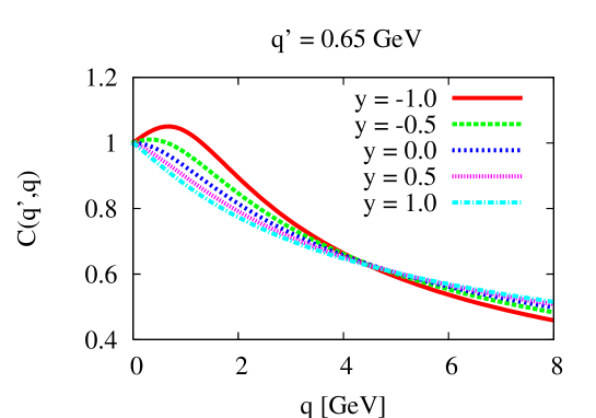
Figure 1: (Color online) The momentum and angle dependence of the function $C({\mathbf{q}}^{\prime},{\mathbf{q}})$ from Eq. (100) at fixed momentum $q^{\prime}$ = 0.65 GeV.

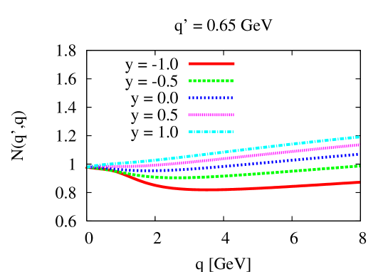
Figure 2: (Color online) The momentum and angle dependence of the function $N({\mathbf{q}}^{\prime},{\mathbf{q}})$ from Eq. (99) at fixed momentum $q^{\prime}$ = 0.65 GeV.

These permutation operators, which change the order of coupling, are essentially Racah coefficients for the Poincaré group. In the nonrelativistic case the functions $N({\mathbf{q}}^{\prime},{\mathbf{q}})$ and $C({\mathbf{q}}^{\prime},{\mathbf{q}})$ both reduce to the constant 1 and have the relatively compact form of the matrix elements of $P$ given in e.g. bound3d ; scatter3d . Since both functions depend on magnitudes as well as angles between the momentum vectors, the 3D formulation is very appropriate for our relativistic calculations. In order to illustrate the momentum and angle dependence we display in Fig. 1 the function $C({\mathbf{q}}^{\prime},{\mathbf{q}})$ for a given value of $|{\bf q^{\prime}}|$ = 0.65 GeV as function of $|{\bf q}|$ and several values of the angle $y={\bf\hat{q}^{\prime}}\cdot{\bf\hat{q}}$. In general the values of $C$ drop below 1 as $q$ increases. The angle dependence is strongest for small $q$, where for ${\bf\hat{q}^{\prime}}\cdot{\bf\hat{q}}=-1$ the function is larger than 1. For the same fixed value of $|{\bf q^{\prime}}|$ we display the function $N({\mathbf{q}}^{\prime},{\mathbf{q}})$ in Fig. 2. Here we see a slowly varying dependence on the momentum $|{\bf q}|$ and a strong angle dependence. For small angles ($y=1$) the function $N({\bf q}^{\prime},{\bf q})$ is larger than 1, whereas for large angles ($y=-1$) it is reduced from 1 by as much as 20%.

In matrix form the Faddeev equation, Eq. (79), has the form

$$\langle\mathbf{k},\mathbf{q}\|T\|\varphi_{d},\mathbf{q}_{0}\rangle=\langle\mathbf{k},\mathbf{q}\|T_{1}P\|\varphi_{d},\mathbf{q}_{0}\rangle+\langle\mathbf{k},\mathbf{q}\|T_{1}P(z-M_{0})^{-1}T\|\varphi_{d},\mathbf{q}_{0}\rangle.$$ (101)

Since at this stage we are only carrying out first order calculations, we only need to consider the first term. Explicitly this is given as

$$\langle\mathbf{k},\mathbf{q}\|T({\sf W})\|\varphi_{d},\mathbf{q}_{0}\rangle = \langle\mathbf{k},\mathbf{q}\|T_{1}(\mathbf{q},\varepsilon)P\|\varphi_{d},\mathbf{q}_{0}\rangle$$ (102)

$$= \int{d\mathbf{k}^{\prime}d\mathbf{q}^{\prime}d\mathbf{k}^{\prime\prime}d\mathbf{q}^{\prime\prime}\langle\mathbf{k},\mathbf{q}\|T_{1}(\mathbf{q},\varepsilon)\|\mathbf{k}^{\prime},\mathbf{q}^{\prime}\rangle\langle\mathbf{k}^{\prime},\mathbf{q}^{\prime}\|P\|\mathbf{k}^{\prime\prime},\mathbf{q}^{\prime\prime}\rangle\langle\mathbf{k}^{\prime\prime},\mathbf{q}^{\prime\prime}|\varphi_{d},\mathbf{q}_{0}\rangle}$$

$$= \int d{\mathbf{k}}^{\prime}d\mathbf{q}^{\prime}d\mathbf{k}^{\prime\prime}d\mathbf{q}^{\prime\prime}\;T_{1}(\mathbf{k},\mathbf{k}^{\prime},\mathbf{q};\varepsilon)\delta(\mathbf{q}^{\prime}-\mathbf{q})\varphi_{d}(\mathbf{k}^{\prime\prime})\delta(\mathbf{q}^{\prime\prime}-\mathbf{q}_{0})$$

$$\times N(\mathbf{q}^{\prime},\mathbf{q}^{\prime\prime})[\delta(\mathbf{k}^{\prime}-\mathbf{k}(\mathbf{q}^{\prime\prime},-\mathbf{q}^{\prime}-\mathbf{q}^{\prime\prime}))\delta(\mathbf{k}^{\prime\prime}+\mathbf{k}(\mathbf{q}^{\prime},-\mathbf{q}^{\prime}-\mathbf{q}^{\prime\prime}))$$

$$+\delta(\mathbf{k}^{\prime}+\mathbf{k}(\mathbf{q}^{\prime\prime},-\mathbf{q}^{\prime}-\mathbf{q}^{\prime\prime}))\delta(\mathbf{p}^{\prime\prime}-\mathbf{p}(\mathbf{q}^{\prime},-\mathbf{q}^{\prime}-\mathbf{q}^{\prime\prime}))]$$

$$= N(\mathbf{q},\mathbf{q}_{0})\;T_{s}\left(\mathbf{p},\mathbf{q}_{0}+\frac{1}{2}\mathbf{q}\>C(\mathbf{q}_{0},\mathbf{q}),\mathbf{q};\varepsilon\right)\varphi_{d}\left(\mathbf{q}+\frac{1}{2}\mathbf{q}_{0}\>C(\mathbf{q},\mathbf{q}_{0})\right).$$

Here the invariant parametric energy $\varepsilon$ which enters the two-body t-matrix is given by $\varepsilon=W-\sqrt{m^{2}+\mathbf{q}^{2}}$. Since we consider bosons, the symmetrized two-body transition matrix $T_{s}$ is given by

$$T_{s}(\mathbf{k},\mathbf{k}^{\prime},\mathbf{q};\varepsilon) = T_{1}(\mathbf{k},\mathbf{k}^{\prime},\mathbf{q};\varepsilon)+T_{1}(-\mathbf{k},\mathbf{k}^{\prime},\mathbf{q};\varepsilon)$$ (103)

$$= T_{1}(\mathbf{k},\mathbf{k}^{\prime},\mathbf{q};\varepsilon)+T_{1}(\mathbf{k},-\mathbf{k}^{\prime},\mathbf{q};\varepsilon).$$

This expression is the starting point for our numerical calculations of the transition amplitude in first order. The first step for an explicit calculation is the selection of independent variables. Since we ignore spin and iso-spin dependencies, the matrix element $\langle{\bf k},{\bf q}\|T\|\varphi_{d},{\bf q_{0}}\rangle$ is a scalar function of the variables $\mathbf{k}$ and $\mathbf{q}$ for a given projectile momentum $\mathbf{q}_{0}$. Thus one needs 5 variables to uniquely specify the geometry of the three vectors $\mathbf{k}$, $\mathbf{q}$ and $\mathbf{q}_{0}$. We follow here the procedure from Ref. scatter3d and choose as variables

$$k=|{\mathbf{k}}|,\ q=|{\mathbf{q}}|,\ x_{k}=\hat{{\mathbf{k}}}\cdot\hat{{\mathbf{q}}}_{0},\ x_{q}=\hat{{\mathbf{q}}}\cdot\hat{{\mathbf{q}}}_{0},\ x^{q_{0}}_{kq}=\widehat{({\mathbf{q}}_{0}\times{\mathbf{q}})}\cdot\widehat{({\mathbf{q}}_{0}\times{\mathbf{k}})}.$$ (104)

The last variable, $x^{q_{0}}_{kq}$, is the angle between the two normal vectors of the $\mathbf{k}$-$\mathbf{q}_{0}$-plane and the $\mathbf{q}$-$\mathbf{q}_{0}$-plane, which are explicitly given by

$$\widehat{({\mathbf{q}}_{0}\times{\mathbf{k}})} = \frac{\hat{\mathbf{q}}_{0}\times\hat{\mathbf{k}}}{\sqrt{1-(\hat{\mathbf{q}}_{0}\cdot\hat{\mathbf{k}})^{2}}},$$

$$\widehat{({\mathbf{q}}_{0}\times{\mathbf{q}})} = \frac{\hat{\mathbf{q}}_{0}\times\hat{\mathbf{q}}}{\sqrt{1-(\hat{\mathbf{q}}_{0}\cdot\hat{\mathbf{q}})^{2}}}.$$ (105)

With these definitions of variables the expression for the transition amplitude as function of the 5 variables from Eq. (104) has the same form as its nonrelativistic counterpart, and we can apply the algorithm developed in Ref. scatter3d for solving it without partial wave decomposition. The only additional effort is the evaluation of the functions $C(q_{0},q,x_{q})$ and $N(q_{0},q,x_{q})$. However, this is conceptually and numerically quite straightforward, since both functions depend only one angle, $x_{q}$.

VII Two-Body Transition Operator and Relativistic Dynamics

The kinematic effects related to the use of the relativistic Racah coefficients have been described in the previous Section. It is left now, to obtain the transition amplitude of the 2N subsystem embedded in the three-particle Hilbert space , $T_{s}(\mathbf{k},\mathbf{k}^{\prime},\mathbf{q};\varepsilon)$, entering Eq. (102). This is a fully off-shell amplitude depending in addition on the Poincaré-Jacobi momentum ${\bf q}$ of the pair. The embedded 2N transition amplitude satisfies the Lippmann-Schwinger equation

$$T_{1}({\bf k},{\bf k}^{\prime};{\bf q})=V_{1}({\bf k},{\bf k}^{\prime};{\bf q})+\int d{\bf k}^{\prime\prime}\>\frac{V_{1}({\bf k},{\bf k}^{\prime\prime};{\bf q})\>T_{1}({\bf k}^{\prime\prime},{\bf k}^{\prime};{\bf q})}{\sqrt{[2\sqrt{m^{2}+\mathbf{p}^{\prime 2}}]^{2}+\mathbf{q}^{2}}-\sqrt{[2\sqrt{m^{2}+\mathbf{p}^{\prime\prime 2}}]^{2}+\mathbf{q}^{2}}+i\epsilon}.$$ (106)

where the interaction (52) can be expressed in the relativistic Jacobi momenta as Ref. fch

$$V({\bf q})=\sqrt{\left[2\sqrt{m^{2}+\mathbf{k}^{2}}+v\right]^{2}+\mathbf{q}^{2}}\>-\>\sqrt{\left[2\sqrt{m^{2}+\mathbf{k}^{2}}\right]^{2}+\mathbf{q}^{2}}.$$ (107)

For ${\bf q}=0$ this expression reduces to the interaction $v({\bf k},{\bf k}^{\prime})\delta(\mathbf{q}-\mathbf{q}\,^{\prime})$, which is the interaction in the two-nucleon mass operator. In the same limit, Eq. (106) reduces to the familiar Lippmann-Schwinger equation with relativistic kinetic energies.

This matrix element is constructed using the methods outlined in equations (85) and (87). First the matrix element of the right half-shell embedded $t$-operator is evaluated using the two-body half shell transition amplitude where the convention of bh is employed

$$\langle\mathbf{k}|T_{1}(\mathbf{q};z^{\prime})|\mathbf{k}^{\prime}\rangle = \langle\mathbf{k}|V(\mathbf{q})|\mathbf{k}^{\prime(-)}\rangle$$ (108)

$$= \frac{2(E_{k^{\prime}}+E_{k})}{\sqrt{4E_{k^{\prime}}^{2}+\mathbf{q}^{2}}+\sqrt{4E_{k}^{2}+\mathbf{q}^{2}}}t(\mathbf{k},\mathbf{k}^{\prime};2E_{k^{\prime}}),$$

where the 2N transition amplitude $t(\mathbf{k},\mathbf{k}^{\prime};2E_{k^{\prime}})$ is the solution of the half-shell Lippmann-Schwinger equation

$$t(\mathbf{k},\mathbf{k}^{\prime};2E_{k^{\prime}})=v(\mathbf{k},\mathbf{k}^{\prime})+\int d\mathbf{k}^{\prime\prime}\frac{v(\mathbf{k},\mathbf{k}^{\prime\prime})t(\mathbf{k}^{\prime\prime},\mathbf{k}^{\prime};2E_{k^{\prime}})}{E_{k^{\prime}}-2\sqrt{m^{2}+k^{\prime\prime 2}}+i\epsilon}.$$ (109)

This solution is used as input to equation (87) which has the form

$$\langle\mathbf{k}|T_{1}(\mathbf{q};z)|\mathbf{k}^{\prime}\rangle = \langle\mathbf{k}|T_{1}(\mathbf{q};z^{\prime}|\mathbf{k}^{\prime}\rangle\;-$$

$$\int d\mathbf{k}^{\prime\prime} \langle\mathbf{k}|T_{1}(\mathbf{q};z)|\mathbf{k}^{\prime\prime}\rangle\Big{(}\frac{1}{z-\sqrt{4(m^{2}+\mathbf{k}^{\prime\prime 2})+\mathbf{q}^{2}}}-\frac{1}{z^{\prime}-\sqrt{4(m^{2}+\mathbf{k}^{\prime\prime 2})+\mathbf{q}^{2}}}\Big{)}\langle\mathbf{k}^{\prime\prime}|T_{1}(\mathbf{q};z^{\prime})|\mathbf{k}^{\prime}\rangle,$$ (110)

where $T_{1}(z^{\prime})$ is taken to be right half-shell with $z^{\prime}=\sqrt{4(m^{2}+\mathbf{k}^{\prime 2})+\mathbf{q}^{2}}+i\epsilon$. Note that in this equation the unknown matrix element is to the left of the kernel.

We refer to $T_{1}({\bf k},{\bf k}^{\prime};{\bf q}):=\langle\mathbf{k}|T_{1}(\mathbf{q};z)|\mathbf{k}^{\prime}\rangle$ as the embedded 2N t-matrix and to $V({\bf k},{\bf k}\,^{\prime};{\bf q})$ as the embedded interaction. Matrix elements of $T_{1}(z)$ can be alternatively calculated by inserting a complete set of eigenstates of the 2N mass operator $m_{12}=2\sqrt{\mathbf{k}^{2}+m^{2}}+v$, as has been carried out in Ref. reltrit02 for a relativistic calculation of the triton binding energy using two-body s-waves. Similarly, this method of spectral decomposition can be used to directly calculate the matrix elements of the embedded two-body t-matrix, as has been done in another relativistic calculation of the triton binding energy reltrit86 . The general difficulty with this method of spectral decomposition is that it requires an integration over the c.m. half-shell matrix elements $t({\bf k},{\bf k}^{\prime};E_{k^{\prime}})$ in $k^{\prime}$, requiring the knowledge of those matrix elements for large values of $k^{\prime}$, which can pose a challenge with respect to numerical accuracy. To our knowledge, this method has not yet led to a successful relativistic calculation of scattering observables.

We use Eq.(110) to explicitly construct the elements of the fully off-shell t-matrix, which enters the calculation of the three-body transition amplitude given in Eq. (102). For every off-shell momentum $\mathbf{k}^{\prime}$ the integral equation, Eq.(110), must be solved for each $z$. It is worthwhile to note that the $\mathbf{k}^{\prime\prime}$ integration in Eq.(110) only involves momenta of the half-shell t-matrices, but no energies. The momenta $\mathbf{k}$ and $\mathbf{k}^{\prime}$ are fixed by requirements of the three-body calculation, and typically are not higher than 7 GeV. We tested that for converged results the $\mathbf{k}^{\prime\prime}$ integration has to go up to about 12 GeV. The singularities in the two denominators of Eq.(110) do not pose any problems and are handled with standard subtraction techniques.

In order to obtain insight into the impact of the embedding for different values of $\mathbf{q}$, we introduce approximations to the embedded interaction. First, we completely neglect $\mathbf{q}$ in the embedded interaction, which leads to

$$V({\bf k},{\bf k}^{\prime};{\bf q})\to V_{0}({\bf k},{\bf k}^{\prime};{\bf q})=v({\bf k},{\bf k}^{\prime}).$$ (111)

Furthermore, we want to test the leading order terms in a $\mathbf{q}/m$ and $v/m$ expansion as suggested in Ref. witalar1

$$V({\bf k},{\bf k}^{\prime};{\bf q})\to V_{1}({\bf k},{\bf k^{\prime}};{\bf q})=v({\bf k},{\bf k}^{\prime})\left(1-\frac{\mathbf{q}^{2}}{8m^{2}}\right)$$ (112)

and

$$V({\bf k},{\bf k}^{\prime};{\bf q})\to V_{2}({\bf k},{\bf k}^{\prime};{\bf q})=v({\bf k},{\bf k})\left(1-\frac{\mathbf{q}^{2}}{8\sqrt{m^{2}+\mathbf{k}^{2}}\>\sqrt{m^{2}+\mathbf{k}^{\prime 2}}}\right)$$ (113)

and explore their validity as function of projectile energy.

VIII Cross Sections for Elastic Scattering

The calculation of the cross section for elastic scattering, Eq. (92), requires the knowledge of the matrix element $\langle\varphi_{d},{\bf{\hat{q}}},q_{0}|U|\varphi_{d},{\bf q_{0}}\rangle$. Using the definition of the operator $U$, Eq. (78), inserting a complete set of states and using for the matrix elements of the permutation operator the expression from Eq. (98), we obtain

$$\langle\varphi_{d},\mathbf{q}\|U\|\varphi_{d},\mathbf{q}_{0}\rangle = \langle\varphi_{d},\mathbf{q}\|P(z-M_{0})+PT\|\varphi_{d},\mathbf{q}_{0}\rangle$$ (114)

$$= \int{d\mathbf{k}^{\prime}d\mathbf{q}^{\prime}d\mathbf{k}^{\prime\prime}d\mathbf{q}^{\prime\prime}\langle\varphi_{d},\mathbf{q}|\mathbf{k}^{\prime},\mathbf{q}^{\prime}\rangle\langle\mathbf{k}^{\prime},\mathbf{q}^{\prime}\|P\|\mathbf{k}^{\prime\prime},\mathbf{q}^{\prime\prime}\rangle\langle\mathbf{k}^{\prime\prime},\mathbf{q}^{\prime\prime}\|(z-M)+T\|\varphi_{d},\mathbf{q}_{0}\rangle}$$

$$= \left(W-\sqrt{m^{2}+\mathbf{q}_{0}^{2}}-\sqrt{4(m^{2}+(\mathbf{q}+\frac{1}{2}\mathbf{q_{0}}\>C(\mathbf{q},\mathbf{q}_{0}))^{2})+\mathbf{q}_{0}^{2}}\right)$$

$$\times 2N(\mathbf{q},\mathbf{q}_{0})\varphi_{d}\left(\left|\mathbf{q}_{0}+\frac{1}{2}\mathbf{q}\>C(\mathbf{q}_{0},\mathbf{q})\right|\right)\varphi_{d}\left(\left|\mathbf{q}+\frac{1}{2}\mathbf{q}_{0}\>C(\mathbf{q},\mathbf{q}_{0})\right|\right)$$

$$+2\int d^{3}q^{\prime\prime}\;N(\mathbf{q},\mathbf{q}^{\prime\prime})\varphi_{d}\left(\left|\mathbf{q}^{\prime\prime}+\frac{1}{2}\mathbf{q}\>C(\mathbf{q}^{\prime\prime},\mathbf{q})\right|\right)$$

$$\times\>\langle\mathbf{q}+\frac{1}{2}\mathbf{q}^{\prime\prime}\>C(\mathbf{q},\mathbf{q}^{\prime\prime}),\mathbf{q}^{\prime\prime}\|T\|\varphi_{d},\mathbf{q}_{0}\rangle.$$

In first order the transition amplitudes reads $T=tP$, thus the final expression for the transition amplitude for elastic scattering becomes

$$\langle\varphi_{d},\mathbf{q}\|U\|\varphi_{d},\mathbf{q}_{0}\rangle = \left({\sf W}-\sqrt{m^{2}+\mathbf{q}_{0}^{2}}-\sqrt{4[m^{2}+(\mathbf{q}+\frac{1}{2}\mathbf{q}_{0}\>C(\mathbf{q},\mathbf{q}_{0}))^{2}]+\mathbf{q}_{0}^{2}}\right)$$ (115)

$$\times 2N(\mathbf{q},\mathbf{q}_{0})\varphi_{d}\left(\left|\mathbf{q}_{0}+\frac{1}{2}\mathbf{q}\>C(\mathbf{q}_{0},\mathbf{q})\right|\right)\varphi_{d}\left(\left|\mathbf{q}+\frac{1}{2}\mathbf{q}_{0}\>C(\mathbf{q},\mathbf{q}_{0})\right|\right)$$

$$+2\int d\mathbf{q}^{\prime\prime}\;N(\mathbf{q},\mathbf{q}^{\prime\prime})\varphi_{d}\left(\left|\mathbf{q}^{\prime\prime}+\frac{1}{2}\mathbf{q}\>C(\mathbf{q}^{\prime\prime},\mathbf{q})\right|\right)\>\varphi_{d}\left(\left|\mathbf{q}^{\prime\prime}+\frac{1}{2}\mathbf{q}\>C(\mathbf{q}^{\prime\prime},\mathbf{q}_{0})\right|\right)$$

$$\times T_{s}\left(({\bf q}+\frac{1}{2}\mathbf{q}^{\prime\prime}\>C(\mathbf{q},\mathbf{q}^{\prime\prime})),({\bf q}_{0}+\frac{1}{2}\mathbf{q}\>C(\mathbf{q}_{0},\mathbf{q}));\varepsilon\right),$$

where $\varepsilon={\sf W}-\sqrt{m^{2}-\mathbf{q}^{\prime\prime 2}}$.

In the following we want to compare a non-relativistic first order calculation to a corresponding relativistic one. What is common in both calculations is the input two-body interaction. In the relativistic case it is transformed to be two-body scattering equivalent to the non-relativistic two-body calculation. Though we consider only spin-isospin independent interactions, we nevertheless can provide qualitative insights for various cross sections in three-body scattering in the intermediate energy regime, which we define as ranging from 200 MeV to 1 GeV projectile energy. The focus of our investigation will be how kinematic and dynamic relativistic effects manifest themselves at different energies and for different scattering observables.

As model interaction we choose a superposition of two Yukawa interactions of Malfliet-Tjon type malfliet69-1 with parameters chosen such that the potential supports a bound-state, the ‘deuteron’, at -2.23 MeV. The parameters are given in Ref. scatter3d . With this interaction we solve the non-relativistic Faddeev equation in first order as a basis for all comparisons. Then we need to construct a phase equivalent relativistic two-body interaction. We use the procedure suggested by Kamada-Glöckle KG , and obtain a two-body interaction $v({\bf k},{\bf k}^{\prime})$ as Born term of a relativistic two-body Lippmann-Schwinger equation. This two-body t-matrix, $t({\bf k},{\bf k}^{\prime};\varepsilon)$ is the starting point for all calculations which will be presented in the following. In principle there are other methods to obtain a phase-shift equivalent relativistic potential keipo , however in this work we want to focus on the relativistic effects visible in three-body scattering observables, and thus use only one fixed scheme.

Following Ref. witalar1 , as first assessment of the quality of different approximations for the embedded interaction we solve the relativistic 2N Schrödinger equation for the deuteron as function of the momentum $|{\bf q}|$, which takes the form

$$\Phi_{d}({\bf k})=\frac{1}{\sqrt{m_{d}^{2}+{\bf q}^{2}}-\sqrt{2E_{k_{m}}^{2}+{\bf q}^{2}}}\;\int d{\bf k}^{\prime}\;V({\bf k},{\bf k}^{\prime};{\bf q})\Phi_{d}({\bf k}^{\prime}).$$ (116)

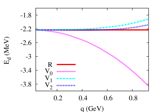
Figure 3: (Color online) The deuteron binding in energy calculated with the embedded interaction $V({\bf k},{\bf p};{\bf q})$ as function of q. The solid line labeled ‘R’ represents the binding energy of -2.23 MeV which is independent of q, when the full embedded interaction is employed. The dotted line is obtained if q is set to zero in the embedded interaction. The dotted, dash-dotted and dashed lines show the approximations to the embedded interaction $V_{0}$, $V_{1}$, and $V_{2}$ as given in Eqs. (111), (112), and (113).

Here $m_{d}$ is the rest mass of the deuteron. In Fig. 3 we show the deuteron binding energy $\varepsilon_{d}$ calculated using the approximations of the embedded interaction given in Eqs. (111), (112), and (113). A correctly embedded interaction should of course not change $\varepsilon_{d}$ at all. We see that $\varepsilon_{d}$ based on the calculation using $V_{0}$ starts to deviate already for very small $q$. The approximation $V_{1}$ gives reasonable results up to $q\approx$ 0.3 GeV, whereas $V_{2}$ is good to about 0.6 GeV. In the following we will see how far these simple estimates are reflected in the calculation of various scattering observables.

As a first observable we consider the total cross section for elastic scattering, $\sigma_{el}$, which is given in Table 1 for projectile kinetic energies from 10 MeV up to 1 GeV. Starting from the non-relativistic cross section, we successively implement different relativistic features to study them in detail. First we only change the phase space factor in the calculation (psf) together with the relativistic transformation from laboratory to c.m. frame, and only then implement the relativistic kinematics due to the Poincaré-Jacobi coordinates (R-kin). The relativistic phase space factor alone has a large effect on the size of the total cross section, as was already observed in ndtotal . The kinematic effects of the Poincaré-Jacobi coordinates have the opposite effect and lower the cross section. However, all kinematic effects taken together increase the total cross section by about 6% at 0.2 GeV and about 40% at 1 GeV. Introducing relativistic dynamic effects into the calculation changes this considerably . The full relativistic calculation (R) lowers the total cross section by about 2% at 0.2 GeV and about 6% at 1 GeV, so that in total the relativistic cross section is smaller than the nonrelativistic one. The approximation $V_{2}$ of Eq. (113) is very good in the energy regime considered, even at 1 GeV its result only deviates by about 2% from the full one. As suggested by the calculations of the deuteron binding energy, the approximation $V_{1}$ of Eq. (112) is still reasonable at 0.2 GeV, but after that starts to become worse.

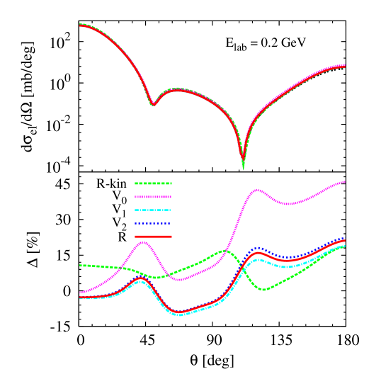
Figure 4: (Color online) The differential cross section for elastic scattering at 0.2 GeV projectile kinetic energy as function of the laboratory scattering angle (upper panel). The solid line represents the fully relativistic calculation. The lower panel shows the relative deviation $\Delta$ with respect to the corresponding non-relativistic calculation. The long-dashed curve labeled ‘R-kin’ represents a calculation in which only relativistic kinematic effects are incorporated. The dotted, dash-dotted, and dashed curves show the approximations to the embedded interaction $V_{0}$, $V_{1}$, and $V_{2}$ as given in Eqs. (111), (112), and (113).

Next we consider the differential cross section for elastic scattering. In Fig. 4 we show the calculation for 0.2 GeV projectile kinetic energy. Since differences between the calculations disappear on a logarithmic scale, we also show the quantity

$$\Delta=\frac{\left(\frac{d\sigma}{d\Omega}\right)_{R}-\left(\frac{d\sigma}{d\Omega}\right)_{NR}}{\left(\frac{d\sigma}{d\Omega}\right)_{NR}}$$ (117)

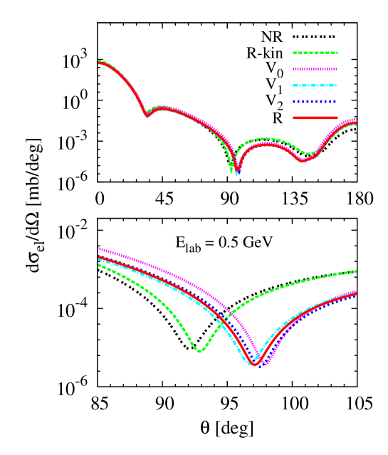
Figure 5: (Color online) The differential cross section for elastic scattering at 0.5 GeV projectile kinetic energy as function of the laboratory scattering angle. The double-dotted curve labeled ‘NR’ represents the non-relativistic calculation, and the solid curve labeled ‘R’ the corresponding fully relativistic one. The long-dashed curve labeled ‘R-kin’ represents a calculation in which only relativistic kinematic effects are incorporated. The dotted, dash-dotted, and dashed curves show the approximations to the embedded interaction $V_{0}$, $V_{1}$, and $V_{2}$ as given in Eqs. (111), (112), and (113).

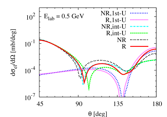
Figure 6: (Color online) The differential cross section for elastic scattering at 0.5 GeV projectile kinetic energy as function of the laboratory scattering angle. The double-dotted curve labeled ‘NR’ represents the non-relativistic calculation, and the solid curve labeled ‘R’ the corresponding fully relativistic one. The two other sets of curves show the contributions from the two different terms contributing to the transition operator $U$ in the non-relativistic (NR) and relativistic (R) calculation. See text for further discussion.

expressed in percentage for the different approximations in the lower panel of Fig. 4. For the backward angles, $\theta\geq 135^{o}$, which correspond to higher momentum transfer, all relativistic effects increase the cross section. Here it can be clearly seen that indeed $V_{0}$ is a bad approximation, whereas $V_{1}$ and $V_{2}$ are of about the same quality. We also see that there is a small difference between the calculation based on $V_{2}$ and the full result. Similar findings, however without the full calculation, were presented in Ref. witalar1 . When going to higher projectile kinetic energies, we expect that the effects increase. This is indeed so, as shown in Fig. 5 for the differential cross section at 0.5 GeV projectile kinetic energy. Here the second minimum in the cross section around 90^o shows a shift towards larger angles once relativistic dynamics is included. This phenomenon has been seen and studied in some electron-deuteron scattering DPSW calculations. To study this shift in more detail we show in the lower panel of Fig. 5 a restricted angular range. Here we can see that the relativistic kinematics produces a shift of the minimum by a few degrees. The magnification shows that the approximations of the embedded interaction oscillate by a few degrees around the full solution. At the extreme backward angles, the relativistic cross section is larger than the non-relativistic one, as was the case at 0.2 GeV. In order to illuminate the details of the two minima of the cross section at 0.5 GeV even further, we show in Fig. 6 the two terms contributing to the operator $U$ for elastic scattering separately. The curves labeled ‘1st-U’ correspond to the first term in Eq. (115) or the operator $P(z-M_{0})$ in Eq. (78), which contributes to the structure of the cross section at backward angles and depends only on the product of two deuteron wave functions evaluated at shifted momenta. Here the relativistic calculation is pushed slightly towards smaller angles indicating the effect of the functions $C({\bf q},{\bf q_{0}})$. The second term in Eq. (115), represented by the curves labeled ‘int-U’, contains in integral over the two-body t-matrix and a product of deuteron wave functions, and basically determines the structure of the cross section for angles up to about 100^o. Here we see the shift of the minimum towards higher angles for the relativistic calculation. The interference of both terms in the calculation gives the final pattern as seen in Fig. 5.

IX Cross Sections for Breakup Processes

The calculation of the breakup cross section, Eq. (91), requires the knowledge of the matrix element $\langle{\bf k},{\bf q}\|U_{0}\|\phi_{d},{\bf q_{0}}\rangle$. Energy conservation requires that in Eq. (91) ${\sf W}_{f}={\sf W}_{i}\equiv{\sf W}=\sqrt{4(m^{2}+k^{2})+q^{2}}+\sqrt{m^{2}+q^{2}}$. This gives a relation between the momenta k and q. In fact, for each given q the magnitude of k is fixed as $k_{a}\equiv|{\mathbf{k}_{a}}|=\frac{1}{2}\sqrt{{\sf W}^{2}-3m^{2}-2{\sf W}\sqrt{m^{2}+q^{2}}}$. This leads to

$$\sigma_{br}^{cm}=\frac{(2\pi)^{4}}{3}\frac{E(q_{0})E_{d}(q_{0})}{q_{0}{\sf W}}\;\int d\Omega_{p}d\Omega_{q}dq\;q^{2}\frac{k_{a}}{4}\sqrt{4(m^{2}+k_{a}^{2})+q^{2}}\;\left|\langle{\mathbf{p}},{\mathbf{q}}\|U_{0}\|\varphi_{d},{\mathbf{q}}_{0}\rangle\right|^{2}$$ (118)

We will consider here the cross sections for two different breakup processes, the inclusive breakup, where only one of the outgoing particles is detected, and the full or exclusive breakup. In order to obtain the differential cross section for inclusive breakup, one still needs to integrate over the solid angle of the undetected particle to arrive at invariant cross section:

$$\frac{d^{3}\sigma_{br}^{cm}}{d\Omega_{q}dE_{q}}=\frac{(2\pi)^{4}}{3}\frac{E(q_{0})E_{d}(q_{0})E(q)q}{q_{0}{\sf W}}\;\int d\Omega_{k}\frac{k_{a}}{4}\sqrt{4(m^{2}+k_{a}^{2})+q^{2}}\;\left|\langle\mathbf{k},\mathbf{q}\|U_{0}\|\varphi_{d},\mathbf{q}_{0}\rangle\right|^{2}.$$ (119)

Here we changed from the variable $dq$ to the more utilized $dE_{q}$. The five-fold differential cross section for exclusive scattering, where both particles are detected, is given by

$$\frac{d^{5}\sigma_{br}^{cm}}{d\Omega_{k}d\Omega_{q}dE_{q}}=\frac{(2\pi)^{4}}{3}\frac{E(q_{0})E_{d}(q_{0})E(q)\;q}{q_{0}{\sf W}}\;\frac{p_{a}}{4}\sqrt{4(m^{2}+k_{a}^{2})+q^{2}}\;\left|\langle\mathbf{k},\mathbf{q}\|U_{0}\|\varphi_{d},\mathbf{q}_{0}\rangle\right|^{2}.$$ (120)

Next we need to explicitly evaluate the matrix element for breakup scattering, $\langle\mathbf{k},\mathbf{q}\|U_{0}\|\varphi_{d},\mathbf{q}_{0}\rangle$, with $U_{0}$ given in Eq. (78)

$$\langle\mathbf{k},\mathbf{q}\|U_{0}\|\varphi_{d},\mathbf{q}_{0}\rangle=\langle\mathbf{k},\mathbf{q}\|T\|\varphi_{d},\mathbf{q}_{0}\rangle+\langle\mathbf{k},\mathbf{q}\|P_{12}P_{23}T\|\varphi_{d},\mathbf{q}_{0}\rangle+\langle\mathbf{k},\mathbf{q}\|P_{13}P_{23}T\|\varphi_{d},\mathbf{q}_{0}\rangle.$$ (121)

The two terms containing the permutations can be calculated analytically, as we show explicitly for the second term using the expressions of Eqs. (95) and (97) for the Poincaré-Jacobi coordinates

$$\langle\mathbf{k},\mathbf{q}\|P_{12}P_{23}T\|\varphi_{d},\mathbf{q}_{0}\rangle$$ (122)

$$= \int d{\bf q_{1}}d{\bf q}_{2}d{\bf q}_{3}\int d{\bf k^{\prime}}d{\bf q^{\prime}}\langle\mathbf{k},\mathbf{q}|\mathbf{q}_{1},\mathbf{q}_{2},\mathbf{q}_{3}\rangle\langle\mathbf{q}_{1},\mathbf{q}_{2},\mathbf{q}_{3}\|P_{12}P_{23}\|\mathbf{k}^{\prime},\mathbf{q}^{\prime}\rangle\langle\mathbf{k}^{\prime},\mathbf{q}^{\prime}\|T\|\varphi_{d},\mathbf{q}_{0}\rangle$$

$$= \int d{\bf q_{1}}d{\bf q}_{2}d{\bf q}_{3}\int d{\bf k^{\prime}}d{\bf q^{\prime}}\delta(\mathbf{q}_{1}+\mathbf{q}_{2}+\mathbf{q}_{3}-\mathbf{P})\;{\hat{n}}({\bf q}_{1};{\bf q}_{2},{\bf q}_{3})\;{\hat{n}}({\bf q}_{2};{\bf q}_{3},{\bf q}_{1})$$

$$\times\delta(\mathbf{q}-\mathbf{q}_{1})\;\delta(\mathbf{k}-\mathbf{k}_{23})\;\delta(\mathbf{q}^{\prime}-\mathbf{q}_{2})\;\delta(\mathbf{k}^{\prime}-\mathbf{k}_{31})\langle\mathbf{k}^{\prime},\mathbf{q}^{\prime}\|T\|\varphi_{d},\mathbf{q}_{0}\rangle.$$

Taking particle 1 as spectator we can evaluate the momenta ${\bf q}_{i}$ explicitly as

$$\mathbf{q}_{1} = \mathbf{q}$$

$$\mathbf{q}_{2} = \mathbf{k}-\frac{\mathbf{q}}{2E(k)}\left(\frac{-\mathbf{k}\cdot\mathbf{q}}{\sqrt{(2E(k))^{2}+q^{2}}+2E(k)}+E(k)\right)$$

$$\mathbf{q}_{3} = -\mathbf{k}-\frac{\mathbf{q}}{2E(k)}\left(\frac{\mathbf{k}\cdot\mathbf{q}}{\sqrt{(2E(k))^{2}+q^{2}}+2E(k)}+E(k)\right).$$ (123)

From this ${\bf q}^{\prime}$ and ${\bf k}^{\prime}$ can be obtained as ${\bf q}^{\prime}={\bf q}_{3}$ and ${\bf k}^{\prime}={\bf k}_{31}$ by inserting the expressions of Eq. (123) into Eq. (95) leading to

$$\langle\mathbf{k},\mathbf{q}\|P_{12}P_{23}T\|\varphi_{d},\mathbf{q}_{0}\rangle={\hat{n}}({\bf q}_{1};{\bf q}_{2}{\bf q}_{3})\;{\hat{n}}({\bf q}_{2};{\bf q}_{3}{\bf q}_{1})\langle{\bf k}_{31},{\bf q}_{2}\|T\|\varphi_{d},\mathbf{q}_{0}\rangle.$$ (124)

In first order we have $T=tP$, and an explicit evaluation leads to

$$\langle\mathbf{k},\mathbf{q}\| P_{12}P_{23}T \|\varphi_{d},\mathbf{q}_{0}\rangle=$$ (125)

$${\hat{n}}({\bf q}_{1};{\bf q}_{2}{\bf q}_{3})\;{\hat{n}}({\bf q}_{2};{\bf q}_{3}{\bf q}_{1})\;N({\bf q}_{2},{\bf q}_{0})\;T_{s}\left({\bf k}_{31},{\bf q}_{0}+\frac{C({\bf q}_{0},{\bf q}_{2})}{2}{\bf q}_{2};\varepsilon\right)\;\varphi_{d}\left({\bf q}_{2}+\frac{C({\bf q}_{2},{\bf q}_{0})}{2}{\bf q}_{0}\right).$$

The functions $N({\bf q}_{2},{\bf q}_{0})$ and $C({\bf q}_{0},{\bf q}_{2})$ are defined in Eqs. (99) and (100). The last term in Eq. (121), $\langle\mathbf{k},\mathbf{q}\|P_{13}P_{23}T\|\varphi_{d},\mathbf{q}_{0}\rangle$, is calculated analogously. Having calculated the matrix element of $U_{0}$, Eq. (121), we can obtain the differential cross section for inclusive as well as exclusive breakup scattering. The expressions for the invariant cross sections in the laboratory variables are derived in Appendix B.

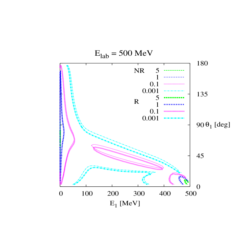
Figure 7: (Color online) The inclusive cross section at 0.5 GeV laboratory projectile kinetic energy as function of the energy $E$ of the emitted particle and its emission angle $\theta$. The angles above the thin dashed line for larger energies and angles are kinematically forbidden. The thin lines represent the contours of the non-relativistic calculation, whereas the thick lines represent the corresponding contours of the relativistic calculation.

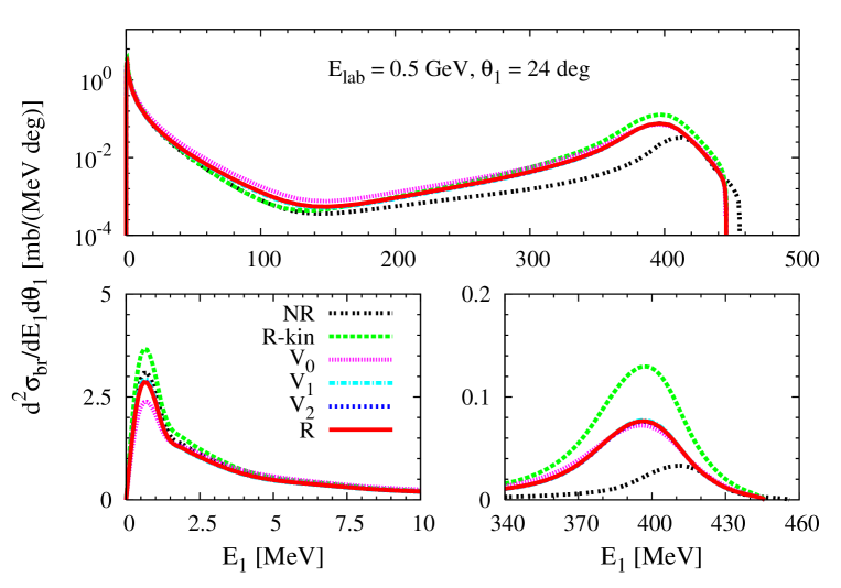
Figure 8: (Color online) The inclusive cross section at 0.5 GeV laboratory projectile kinetic energy as function of the energy $E$ of the emitted particle and a 24^o emission angle. The upper panel displays the entire energy range of the emitted particle, whereas the two lower panels show only the low and the high energies in a linear scale. The solid line represents the fully relativistic calculation, the double-dotted line the corresponding non-relativistic one. The long-dashed curve labeled ‘R-kin’ represents a calculation in which only relativistic kinematic effects are incorporated. The dotted, dash-dotted, and dashed curves show the approximations to the embedded interaction $V_{0}$, $V_{1}$, and $V_{2}$ as given in Eqs. (111), (112), and (113).

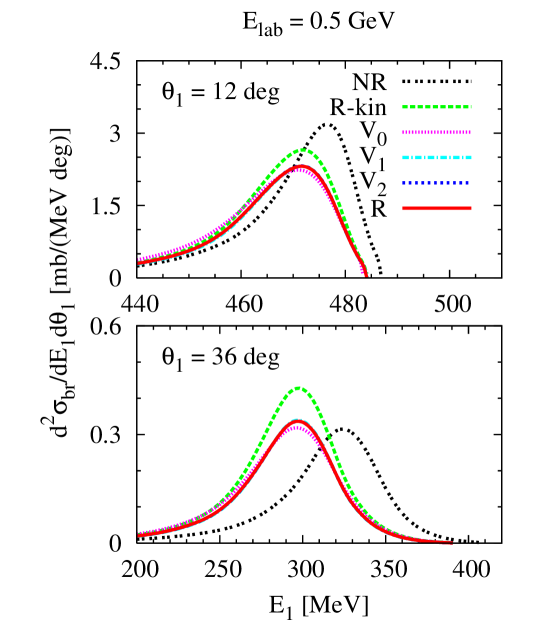
Figure 9: (Color online) Same as Fig. 8 but for different fixed angles of the emitted particle.

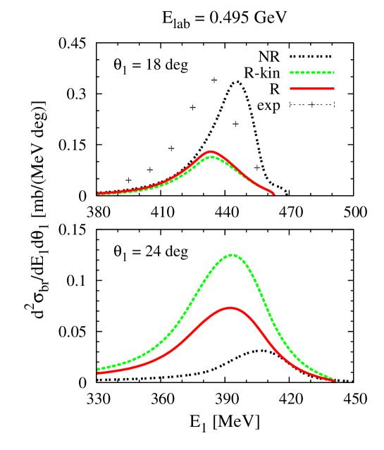
Figure 10: (Color online) The inclusive cross section at 0.495 GeV laboratory projectile kinetic energy as function of the energy $E$ of the emitted particle and fixed emission angles of 18^o and 24^o degrees. The solid line represents the fully relativistic calculation and the double-dotted line the non-relativistic one. The long-dashed curve labeled ‘R-kin’ represents a calculation in which only relativistic kinematic effects are incorporated. The data are from Ref. chen .

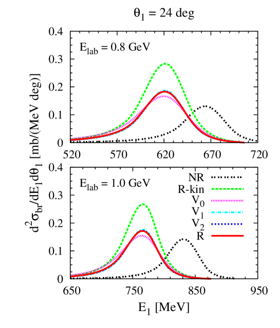
Figure 11: (Color online) The inclusive cross section at 0.8 GeV (upper panel) and 1 GeV (lower panel) laboratory projectile kinetic energy as function of the energy $E$ of the emitted particle and the fixed emission angle of 24^o degrees. The notation of the curves is the same as in Fig. 9.

First, we consider inclusive breakup scattering and compare the cross sections for a non-relativistic first-order calculation in the two-body $t$-operator with the corresponding relativistic one. One can expect that the evaluation of the delta function in the cross section, Eq. (72) will have a substantial effect on breakup cross sections, since it fixes the relation between the magnitudes of the vectors k and q. This in turn determines the maximum allowed kinetic energy the ejected particle is allowed to have as function of the emission angle. To get a global impression of those differences Fig. 7 shows a contour plot of the differential cross section for inclusive breakup scattering as function of the kinetic energy and the emission angle of the ejected particle for the non-relativistic and the fully relativistic calculation. The figure shows that for each angle the maximum allowed kinetic energy of the ejectile is shifted in the relativistic calculation towards smaller values compared to the non-relativistic calculation. Specifically, one can expect a shift of the quasi-free scattering (QFS) peak usually studied in inclusive breakup scattering experiments. In Figs. 8 and 9 we present specific cuts at different constant angles to study details of the calculation. The upper panel of Fig. 8 shows the entire energy range of the ejectile at emission angle $\theta_{1}$ = 24^o in a logarithmic scale, while the lower two panels give a close-up of both peaks on a linear scale. The QFS peak at the large ejectile energy exhibits clearly a shift towards a slightly lower energy compared with the peak position calculated non-relativistically. At this angle, relativistic kinematics given by the phase-space factor and the Poincaré-Jacobi coordinates and indicated by the line labeled ‘R-kin’ results in a peak height, which is almost double that of the full relativistic calculation shown as solid line labeled ‘R’. For breakup scattering we also study the different approximations to the full calculation as introduced in Section IV. In the QFS peak, which is defined by the condition that one of the particles is at rest, even the crudest approximation $V_{0}$, Eq. (111), is very close to the full calculation, the approximations $V_{1}$ and $V_{2}$ are indistinguishable. This is not surprising, since having one particle at rest means that the remaining two are almost in their own c.m. frame, thus ‘boost’ effects should be extremely small. Note that we work here in the total c.m. frame. It is quite illuminating to consider the second peak at very small ejectile kinetic energies. Since the energy of the particle is very small, it should become essentially non-relativistic. This is indeed the case, and the full relativistic calculations almost coincides with the non-relativistic one. It is worthwhile to note that neither relativistic kinematics alone nor the approximation $V_{0}$, which neglects the dependence of the embedded interaction on the pair-momentum is close to the non-relativistic and full relativistic calculations. However, an approximate consideration of this dependence as given by $V_{1}$ or $V_{2}$ seems to suffice. We found that this behavior is similar for low energy ejectiles, independent if the energy of the projectile is 0.5 GeV or 1 GeV. In Fig. 9 we show the QFS peak for two different angles in order to convey that the increase or decrease of the height of the peak depends on the emission angle under consideration. In Fig. 10 we show the QFS peak calculated for a projectile energy of 0.495 GeV and emission angles of 18^o and 24^o, since there is experimental information available for one of the angles. Here we see that the relativistic calculation puts the peak at a position consistent with the data. Since we only carry out a first order calculation with a model potential, we are not surprised that the height of the peak is not described. A similar observation concerning the peak position was already made in Ref. Fachrud , where a first order calculation with two realistic NN interactions was carried out. To give an indication how the position of the QFS peak shifts with increasing projectile energy, we show in Fig. 11 the inclusive cross section for an emission angle of 24^o for projectile energies 0.8 GeV and 1.0 GeV. We see again that in the QFS regime the approximations $V_{1}$ and $V_{2}$ are essentially indistinguishable from the full calculation. Considering only effects of relativistic kinematics results in a peak height double as large as the full calculation, indicating that dynamic effects are very important at those high projectile energies.

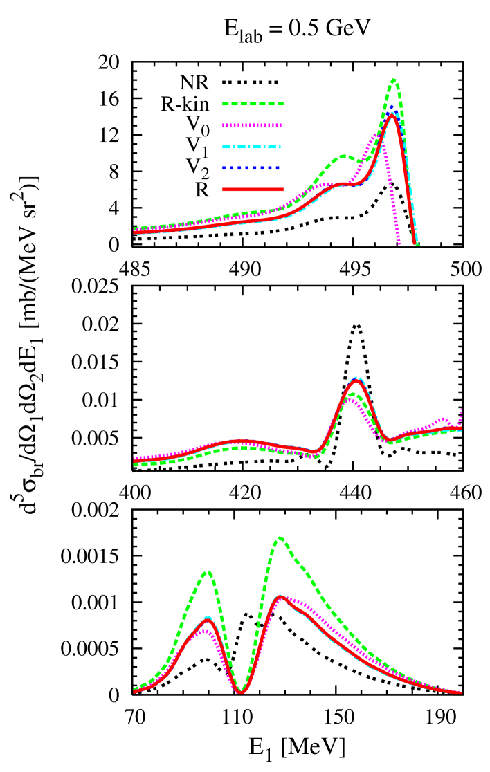
Figure 12: (Color online) The exclusive breakup cross section at 0.5 GeV projectile kinetic energy as function of the ejected particle kinetic energy for three different configurations defined in the three-body c.m. frame. For all configurations the angle $\phi_{pq}$ is 0^o. For the upper panel the cos of the angle between q and the beam ${\bf q_{0}}$ is $x_{q}=1$, i.e. the scattering occurs along the beam line, in the middle panel $x_{q}=\sqrt{3}/2$ and in the lower panel $x_{q}=-0.25$. The cos of the angle between p and ${\bf q_{0}}$ is in the upper panel $x_{p}=0$, in the middle panel $x_{p}=-0.5$ and in the lower panel $x_{p}=-0.9$.

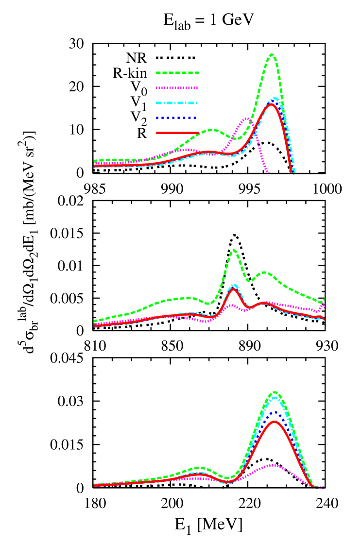
Figure 13: (Color online) Same as Fig.12 but for projectile energy 1.0 GeV.

When considering exclusive breakup one faces many possible configurations that could be considered. Since we are carrying out a model study, we only want to show three specific configurations at two selected energies, 0.5 GeV and 1 GeV in Figs. 12 and 13. In all three configurations the angle $\phi_{kq}$ between the projections of the vectors q and k into the plane perpendicular to the beam direction ${\bf q_{0}}$ is zero. Naive expectation is that when considering scattering in first order in the $t$-operator the probability that one of the particles is scattered along the beam is large. That is indeed the case as shown in the upper panels of Figs. 12 and 13, depicting a so called collinear configuration in which the angle between the vector q and the beam direction ${\bf q_{0}}$ is zero (${\hat{\bf q}}\cdot{\bf{\hat{q}}_{0}}\equiv x_{q}=1$) and the angle between the vector p and the beam direction is 90^o (${\hat{\bf k}}\cdot{\bf{\hat{q}}_{0}}\equiv x_{k}=0$). Once the collinear condition is no longer fulfilled, the cross section becomes considerably smaller, as can be seen in the middle and lower panels of Figs. 12 and 13. For the middle panels the angles are given by $x_{q}=\sqrt{3}/2$ and $x_{p}=-0.5$, for the lower panels they are $x_{q}=-0.25$ and $x_{k}=-0.9$. All configurations in Figs. 12 and 13 show considerable difference between the nonrelativistic and relativistic calculations. At 1 GeV we were specifically looking for possible configurations where the approximations $V_{1}$ and $V_{2}$ of Eqs. (112) and (113) are not close to the full relativistic calculation any longer. Considering the two-body binding energy displayed in Fig. 3, on should expect that the approximation $V_{2}$ can exhibit deviations from the full result at 1 GeV. One such configuration is shown in the lower panel of Fig. 13, where there is a big difference between the calculation with $V_{1}$ and the full result and a discernible difference between the calculation based on $V_{2}$ and the full result. However, we note, that in the majority of configurations where the cross section is still relatively large, $V_{2}$ is still a very good approximation at 1 GeV. Looking at the same configuration at 0.5 GeV, $V_{2}$, and even $V_{1}$ are extremely good approximations to the full result.

X Summary and Conclusions

We investigated relativistic three-nucleon scattering with spinless interactions in the framework of Poincaré invariant quantum mechanics. Since that framework is not widely used in the nuclear physics few-body community we thought it adequate to discuss the formulation of that scheme in some detail, as well as the formulation of scattering theory in this framework. The main points are the construction of unitary irreducible representations of the Poincaré group, both for noninteracting particles as well as for interacting ones. The Poincaré interacting dynamics is constructed by adding an interaction to the noninteracting mass operator which commutes with and is independent of the total linear momentum and the z-component of the total spin.

In this work we do not use partial waves but rather internal vector variables. This leads to what we call Poincaré-Jacobi momenta. They Wigner rotate under kinematic Lorentz transformations of the underlying single particle momenta. In the interacting three-body mass operator the two-body interactions are embedded in the three-particle Hilbert space and are given as fch

$$V_{ij}:=M_{ij}-M_{0}=\sqrt{(m_{0,ij}+v_{ij})^{2}+\mathbf{q}_{k}^{2}}-\sqrt{m_{0,ij}^{2}+\mathbf{q}_{k}^{2}}.$$ (126)

This expression shows explicitly the dependence on the total momentum of the two-body system. For the sake of completeness we also discuss the multichannel scattering theory in that relativistic framework and established the manifestly invariant form of the differential cross section.

The application to three-body scattering is based on the Faddeev scheme, which is reformulated relativistically working with various types of mass operators. The usage of the Poincaré-Jacobi momenta leads to algebraic modifications of corresponding standard nonrelativistic expressions, like e.g. the momentum representation of the permutation operator, Jacobians for the transitions between individual Jacobi momenta. Due to the dependence on the total momentum of the two-body interaction embedded in the three-body system, the two-body off-shell t-operator entering the Faddeev equation acquires additional momentum dependence beyond the usual energy shift which is characteristic in nonrelativistic calculations. This two-body t-operator is then evaluated by expressing it exactly in terms of the solution of half-shell Lippmann-Schwinger equations for a given two-body force in its c.m. frame. We also solve the relativistic Lippmann-Schwinger equation for three different momentum dependent two-body forces, which are approximations to the relativistic embedded interaction.

In order to compare a nonrelativistic calculation to a relativistic one, scattering equivalent two-body forces in the relativistic and nonrelativistic formulations have to be used. In this work we follow the KG prescription to arrive at scattering equivalent two-body forces. There are different schemes, and a detailed study on differences between those schemes will be subject of a forthcoming work. We also restrict ourselves to a first order calculation in the two-body t-operator, which however, already exhibits most of the new relativistic ingredients , both kinematically and dynamically. The two-body force was chosen as a superposition of two Yukawas of Malfliet-Tjon type supporting a bound state, the deuteron, at -2.23 MeV. We calculate three-body scattering observables in the intermediate energy regime, which we take to range from 0.2 GeV to 1 GeV. Those observables are cross sections for elastic as well as breakup scattering, namely inclusive and exclusive scattering. Not surprisingly we find that the difference between nonrelativistic and relativistic calculations increase with increasing energy. This is specifically apparent when looking at the positions of minima in the differential cross section as well positions of QFS peaks in inclusive scattering. When studying various approximations to the relativistic embedded interaction, we find that if the approximations contain terms proportional to the first order in a $p/m$ and $q/m$ expansion, the approximation captures the features of the exact relativistic calculation very well. Only at 1 GeV we start to find discernible deviations in selected configurations for exclusive scattering. Our results clearly indicate an interesting interplay of kinematically and dynamically relativistic effects, which as expected, increase with energy. For example, the total cross section is increased by kinematical effects, whereas the dynamical effects resulting from the q-dependence of the embedded two-body force decrease it. This tendency is also seen in the height of the QFS peak where in most cases the full calculation is lower than the one allowing only for relativistic kinematic effects. Thus, considering only relativistic kinematic effects leads in general to an over prediction of cross sections, which becomes more dramatic the higher the projectile energy is.

The Poincaré invariant relativistic framework is formally close to the nonrelativistic one and therefore standard nonrelativistic formulations, in our case the Faddeev scheme, can be used with proper modifications. The present restriction to a first order calculation in the t-operator will soon be replaced by a complete solution of the corresponding relativistic Faddeev equation following scatter3d , where the nonrelativistic Faddeev equation has been successfully solved employing vector variables. The application to the realistic world of pd scattering at the energies up to 1 GeV considered in this study requires of course two-and three-nucleon forces high above the pion production threshold. Though they are not yet available, they can also be included in the framework of Poincaré invariant quantum mechanics.

Appendix A Invariance of $S$ and relation to $T$

The expression (72) and (73) for the differential cross section can be rewritten in a manifestly invariant form. We write them as a product of an invariant phase space factor, an invariant factor that includes the relative speed, and an invariant scattering amplitude.

To identify and establish the invariance of the invariant scattering amplitude note that the scattering operator $S$ is Poincaré invariant:

$$U_{0}(\Lambda,a){\hat{S}} = U_{0}(\Lambda,a)\Omega_{+}^{\dagger}(H,H_{0})\Omega_{-}(H,H_{0})=\Omega_{+}^{\dagger}(H,H_{0})U(\Lambda,a)\Omega_{-}(H,H_{0})$$ (127)

$$= \Omega_{+}^{\dagger}(H,H_{0})\Omega_{-}(H,H_{0})U_{0}(\Lambda,a)={\hat{S}}U_{0}(\Lambda,a).$$

The Poincaré invariance of the $S$ operator above is a consequence of the intertwining relations for the wave operators

$$U(\Lambda,a)\Omega_{\pm}(H,H_{0})=\Omega_{\pm}(H,H_{0})U_{0}(\Lambda,a)$$ (128)

To show the intertwining property of the wave operators first note that the invariance principle gives the identity

$$\Omega_{\pm}(H,H_{0})=\Omega_{\pm}(M,M_{0}).$$ (129)

The mass operator intertwines by the standard intertwining properties of wave operators. For our choice of irreducible basis the intertwining of the full Poincaré group follows because all of the generators can be expressed as functions of the mass operator and a common set of kinematic operators, $\{\mathbf{K},j_{z},j_{x},j^{2},-i\mbox{\boldmath$\nabla$}_{K}\}$, that commute with the wave operators.

The covariance of the $S$ matrix elements follows from the Poincaré invariance of the $S$ operator if the matrix elements of $S$ are computed in a basis with a covariant normalization.

The $S$-matrix elements can be evaluated in the channel mass eigenstates. After some algebra one obtains:

$$\langle\beta|S_{ba}|\alpha\rangle = \lim_{\tau\to\infty}\langle\beta|e^{iM_{\beta}\tau}e^{-2iM\tau}e^{iM_{\alpha}\tau}|\alpha\rangle$$ (130)

$$= \langle\beta|\alpha\rangle+\lim_{\tau\to\infty}\int_{0}^{\tau}d\tau^{\prime}\,{d\over d\tau^{\prime}}\langle\beta|e^{i({\sf W}_{\beta}+{\sf W}_{\alpha}-2M)\tau^{\prime}}|\alpha\rangle$$

$$= \langle\beta|\alpha\rangle\lim_{\epsilon\to 0^{+}}\left[{2i\epsilon\over{\sf W}_{\beta}-{\sf W}_{\alpha}+2i\epsilon}\right]$$

$$+\lim_{\epsilon\to 0^{+}}\left[{-4i\epsilon\over({\sf W}_{\beta}-{\sf W}_{\alpha})^{2}+4\epsilon^{2}}\right]\langle\beta|\left(V^{\alpha}+V^{\beta}G(\bar{\sf W}+i\epsilon)V^{\alpha}\right)|\alpha\rangle.$$

where $M_{\alpha}|\alpha\rangle={\sf W}_{\alpha}|\alpha\rangle$ and $M_{\beta}|\beta\rangle={\sf W}_{\beta}|\alpha\rangle$ and $\bar{\sf W}:={1\over 2}({\sf W}_{\alpha}+{\sf M}_{\beta})$ is the average invariant mass eigenvalue of the initial and final asymptotic states. In deriving (130) the two strong limits in (58) are replaced a single weak limit. Equation (130) is interpreted as the kernel of an integral operator. $S$-matrix elements are obtained by integrating the sharp eigenstates in Eq. (130) over normalizable functions of the energy and other continuous variables. To simply this expression define the residual interactions $V^{\alpha}$ and $V^{\beta}$ by:

$$V^{\alpha}:=M-M_{\alpha};\qquad V^{\beta}\>=M-M_{\beta},$$ (131)

where

$$V^{\alpha}|\alpha\rangle=(M-{\sf W}_{\alpha})|\alpha\rangle;\qquad V^{\beta}|\beta\rangle=(M-{\sf W}_{\beta})|\beta\rangle.$$ (132)

The resolvent operators of the mass operator and the channel mass operator,

$$G(z):={1\over z-M}\qquad G_{\alpha}(z):={1\over z-M_{\alpha}},$$ (133)

are related by the second resolvent relations Hi :

$$G(z)-G_{\alpha}(z)=G_{\alpha}(z)V^{\alpha}G(z)=G(z)V^{\alpha}G_{\alpha}(z).$$ (134)

It is now possible to evaluate the limit as $\epsilon\to 0$. It is important to remember that this is the kernel of an integral operator.

The first term in square brackets is unity when the initial and final mass eigenvalues are identical, and zero otherwise; however, the limit in the bracket is a Kronecker delta and not a Dirac delta function. For $\alpha\not=\beta$, $\langle\beta({\sf W}^{\prime})|\alpha({\sf W})\rangle$ are Lebesgue measurable in ${\sf W}^{\prime}$ for fixed ${\sf W}$, so there is no contribution from the first term in Eq. (130). For the case that ${\sf W}_{\alpha}={\sf W}_{\beta}$, we have $\langle\beta({\sf W}^{\prime})|\alpha({\sf W})\rangle\propto\delta({\sf W}^{\prime}-{\sf W})$. The matrix element vanishes by orthogonality unless ${\sf W}_{\beta}={\sf W}_{\alpha}$, but then the coefficient is unity. Thus, the first term in (130) is $\langle\beta|\alpha\rangle$ if the initial and final channels are the same, but zero otherwise. The matrix elements also vanish by orthogonality for two different channels governed by the same asymptotic mass operator with the same invariant mass. The first term in (130) therefore includes a channel delta function.

For the second term, the quantity in square brackets becomes $-2\pi i\delta({\sf W}_{\beta}-{\sf W}_{\alpha})$, which leads to the relation

$$\langle\beta|S|\alpha\rangle=\langle\alpha|\beta\rangle-2\pi i\delta({\sf W}_{\beta}-{\sf W}_{\alpha})\langle\beta|T^{\beta\alpha}({\sf W}_{\alpha}+i0^{+})|\alpha\rangle,$$ (135)

where

$$T^{\beta\alpha}(z)=V^{\alpha}+V^{\beta}G(z)V^{\beta}.$$ (136)

and $\langle\alpha|\beta\rangle$ is zero if the initial and final channels are different and is the overlap of the initial and final states if the initial and final channels are the same. Equation (135) is exactly eq. (65).

With our choice of irreducible basis the residual interactions and the resolvent commute with the total linear momentum operator, and if the sharp channel states $|\alpha\rangle$ and $|\beta\rangle$ are simultaneous eigenstates of the appropriate partition mass operator and the linear momentum, then a three-momentum conserving delta function can be factored out of the $T$-matrix element:

$$\langle\beta|T^{\beta\alpha}({\sf W}_{\alpha}+i0^{+})|\alpha\rangle=\delta^{3}(\mathbf{P}_{\beta}-\mathbf{P}_{\alpha})\langle\beta\|T^{\beta\alpha}({\sf W}_{\alpha}+i0^{+})\|\alpha\rangle.$$ (137)

When combined with the three-momentum conserving delta function the invariant mass delta function can be replaced an energy conserving delta function

$$\delta({\sf W}_{\beta}-{\sf W}_{\alpha})=\left|{d{\sf W}\over d{\sf E}}\right|\;\delta({\sf E}_{\beta}-{\sf E}_{\alpha})\qquad\left|{d{\sf W}\over d{\sf E}}\right|={{\sf W}\over{\sf E}}.$$ (138)

The $S$-matrix elements can be expressed in terms of the reduced channel transition operators as follows:

$$\langle\beta|S|\alpha\rangle=\langle\alpha|\beta\rangle\delta_{\beta\alpha}-i(2\pi)\delta^{4}(P_{\beta}-P_{\alpha}){{\sf W}_{\alpha}\over{\sf E}_{\alpha}}\langle\beta\|T^{\beta\alpha}({\sf W}_{\alpha}+i0^{+})\|\alpha\rangle$$ (139)

In this expression the $S$ operator is invariant while the single particle asymptotic states have a non-covariant normalization.

To extract the standard expression for the invariant amplitude the single particle states are replaced by states with the covariant normalization used in the particle data book pdg :

$$|\mathbf{p},\mu\rangle\longrightarrow|p,\mu\rangle_{cov}=|\mathbf{p},\mu\rangle\sqrt{2E_{p_{m}}}(2\pi)^{3/2}.$$ (140)

The resulting expression

$$-i(2\pi)\delta^{4}(P_{\beta}-P_{\alpha}){{\sf W}_{\alpha}\over{\sf E}_{\alpha}}{}_{cov}\langle\beta\|T^{\beta\alpha}({\sf W}_{\alpha}+i0^{+})\|\alpha\rangle_{cov}$$ (141)

is invariant (up to spin transformation properties). Since the four dimensional delta function is invariant, the factor multiplying the delta function is also invariant (up to spin transformation properties). This means that

$${}_{cov}\langle\alpha\|M^{\alpha\beta}\|\beta\rangle_{cov}:={1\over(2\pi)^{3}}{{\sf W}_{\alpha}\over{\sf E}_{\alpha}}{}_{cov}\langle\beta\|T^{\beta\alpha}({\sf W}_{\alpha}+i0^{+})\|\alpha\rangle_{cov}$$ (142)

is a Lorentz covariant amplitude. The factor of $1/(2\pi)^{3}$ is chosen to agree with the normalization convention used in the particle data book pdg .

The differential cross section becomes

$${d\sigma} = {(2\pi)^{4}\over 4E_{m_{t}}(\mathbf{p}_{t})E_{m_{b}}(\mathbf{p}_{b})v_{bt}}\;\left|{}_{cov}\langle p_{1},\cdots,p_{n},\|M^{\alpha\beta}\|\bar{p}_{b},\bar{p}_{t}\rangle_{cov}\right|^{2}$$ (143)

$$\times \delta^{4}\left(\sum_{i}p_{i}-\bar{p}_{b}-\bar{p}_{t}\right)\;{d\mathbf{p}_{1}\over 2E_{m_{1}}(2\pi)^{3}}\cdots{d\mathbf{p}_{n}\over 2E_{m_{n}}(2\pi)^{3}}.$$

The identity

$$v_{bt}={\sqrt{(p_{t}\cdot p_{b})^{2}-m_{b}^{2}m_{t}^{2}}\over E_{m_{b}}E_{m_{t}}}$$ (144)

can be used to get an invariant expression for the relative speed between the projectile and target and

$$d\Phi_{n}({p}_{b}+{k}_{t};\mathbf{p}_{1},\cdots,\mathbf{p}_{n})=\delta^{4}\left(\sum_{i}p_{i}-\bar{p}_{b}-\bar{p}_{t}\right)\;{d\mathbf{k}_{1}\over 2E_{m_{1}}(2\pi)^{3}}\cdots{d\mathbf{k}_{n}\over 2E_{m_{n}}(2\pi)^{3}}$$ (145)

is the standard Lorentz invariant phase space factor. Inserting these covariant expressions in the definition of the differential cross section gives the standard formula for the invariant cross section

$$d\sigma={(2\pi)^{4}\over 4\sqrt{(p_{t}\cdot p_{b})^{2}-m_{b}^{2}m_{t}^{2}}}\left|{}_{cov}\langle p_{1},\cdots,p_{n},\|M^{\alpha\beta}\|\bar{p}_{b},\bar{p}_{t}\rangle_{cov}\right|^{2}d\Phi_{n}({p}_{b}+{p}_{t};\mathbf{p}_{1},\cdots,\mathbf{p}_{n}).$$ (146)

Because of the unitarity of the Wigner rotations and the covariance of $\left|{}_{cov}\langle p_{1},\cdots,p_{n},\|M^{\alpha\beta}\|\bar{p}_{b},\bar{p}_{t}\rangle_{cov}\right|^{2}$ this becomes an invariant if the initial spins are averaged and the final spins are summed.

This manifestly invariant formula for the cross section is identical to (72) and (73); in this form the invariant cross section can be evaluated in any frame. The index $t$ refers to the target, which is in our case the deuteron.

Appendix B Breakup Cross Section in the Laboratory Frame variables

The total breakup cross section is Lorentz invariant. The expression for the differential cross sections (72) is given in terms of single particle variables, while the solutions of the Faddeev equations give transition matrix elements as functions of the Poincaré-Jacobi momenta defined in Section II. To compute the total cross section it is useful to work in a single representation. Since the single particle momenta are directly related to measured parameters of the differential cross section, we change variable in the transition amplitudes from Poincaré Jacobi moment to single particle momenta. In this section the single particle variables are computed in the laboratory frame.

The relation between the product of single particle basis states and states expressed in terms of the Poincaré-Jacobi momenta are given by

$$|\mathbf{p}_{n},\mathbf{p}_{d}\rangle = \left|\frac{\partial(\mathbf{q}_{0},\mathbf{P}_{i})}{\partial(\mathbf{p}_{n},\mathbf{p}_{d})}\right|^{1/2}|\mathbf{q}_{0},\mathbf{P}_{i}\rangle$$

$$|\mathbf{p}_{1},\mathbf{p}_{2},\mathbf{p}_{3}\rangle = \left|\frac{\partial(\mathbf{k},\mathbf{p}_{2}+\mathbf{p}_{3})}{\partial(\mathbf{p}_{2},\mathbf{p}_{3})}\right|^{1/2}\left|\frac{\partial(\mathbf{q},\mathbf{P}_{f})}{\partial(\mathbf{p}_{1},\mathbf{p}_{2}+\mathbf{p}_{3})}\right|^{1/2}|\mathbf{P}_{f},\mathbf{k},\mathbf{q}\rangle$$ (147)

The Jacobians in these transformations are

$$\left|\frac{\partial(\mathbf{q}_{0},\mathbf{P}_{i})}{\partial(\mathbf{p}_{n},\mathbf{p}_{d})}\right| = \frac{E(q_{0})E_{d}(q_{0}){\sf E}_{i}}{E(p_{n})E_{d}(p_{d})W}$$

$$\left|\frac{\partial(\mathbf{k},\mathbf{p}_{2}+\mathbf{p}_{3})}{\partial(\mathbf{p}_{2},\mathbf{p}_{3})}\right| = \frac{\sqrt{(E(k_{2})+E(p_{3}))^{2}-(\mathbf{p}_{2}+\mathbf{p}_{3})^{2}}\;(E(p_{2})+E(p_{3}))}{4E(p_{2})E(p_{3})}$$

$$\left|\frac{\partial(\mathbf{q},\mathbf{P}_{f})}{\partial(\mathbf{p}_{1},\mathbf{p}_{2}+\mathbf{p}_{3})}\right| = \frac{\sqrt{(E(p_{2})+E(p_{3}))^{2}-(\mathbf{p}_{2}+\mathbf{p}_{3})^{2}+\mathbf{q}^{2}}\;E(q){\sf E}_{f}}{E(p_{1})\;(E(p_{2})+E(p_{3}))\;W}$$ (148)

Defining

$$\Gamma(W,\mathbf{k},\mathbf{q})={W^{2}\over{\sf E}_{i}^{2}}\left|\frac{\partial(\mathbf{q}_{0},\mathbf{P}_{i})}{\partial(\mathbf{p}_{n},\mathbf{p}_{d})}\right|\left|\frac{\partial(\mathbf{k},\mathbf{p}_{2}+\mathbf{p}_{3})}{\partial(\mathbf{p}_{2},\mathbf{p}_{3})}\right|\left|\frac{\partial(\mathbf{q},\mathbf{P}_{f})}{\partial(\mathbf{p}_{1},\mathbf{p}_{2}+\mathbf{p}_{3})}\right|,$$ (149)

the total cross section for breakup scattering becomes

$$\sigma_{br}^{lab} = \frac{1}{3}\frac{(2\pi)^{4}}{v_{bt}}\int d\mathbf{p}_{1}d\mathbf{p}_{2}d\mathbf{p}_{3}\;\delta({\sf E}_{f}-{\sf E}_{i})\;\delta^{3}(\mathbf{P}_{f}-\mathbf{P}_{i})\Gamma(W,\mathbf{p},\mathbf{q})\left|\langle\mathbf{p},\mathbf{q}\|U_{0}\|\varphi_{d},\mathbf{q}_{0}\rangle\right|^{2}$$ (150)

$$= \frac{1}{3}\frac{(2\pi)^{4}}{v_{bt}}\int d\mathbf{p}_{1}d\mathbf{p}_{2}\;\delta({\sf E}_{f}-{\sf E}_{i})\Gamma(W,\mathbf{p},\mathbf{q})\left|\langle\mathbf{p},\mathbf{q}\|U_{0}\|\varphi_{d},\mathbf{q}_{0}\rangle\right|^{2},$$

where we used $\mathbf{P}=\mathbf{P}_{i}=\mathbf{P}_{f}$. The $\delta$ function in the energy can be eliminated by a variable change. The total energy of the system is ${\sf E}={\sf E}_{i}={\sf E}_{f}=\sqrt{m^{2}+\mathbf{p}_{1}^{2}}+\sqrt{m^{2}+\mathbf{p}_{2}^{2}}+\sqrt{m^{2}+(\mathbf{P}-\mathbf{p}_{1}-\mathbf{p}_{2})^{2}}$. With $p_{1}\equiv|{\bf p}_{1}|$ and ${\bf{\hat{p}}}_{2}\equiv{\bf p}_{2}/|{\bf p}_{2}|$ this gives

$$\frac{d{\sf E}}{dp_{2}}=\frac{p_{2}}{E(p_{2})}+\frac{p_{2}-(\mathbf{P}-\mathbf{p}_{1})\cdot\hat{\mathbf{p}}_{2}}{{\sf E}-E(p_{1})-E(p_{2})}=\frac{p_{2}({\sf E}-E(p_{1}))-E(p_{2})(\mathbf{P}-\mathbf{p}_{1})\cdot\hat{\mathbf{p}}_{2}}{E(p_{2})E(p_{3})}.$$ (151)

Since $dp_{1}=E(p_{1})/p_{1}dE_{1}$, and $v_{bt}=p_{n}/E(p_{n})$, Eq. (150) becomes

$$\sigma_{br}^{lab}=\frac{(2\pi)^{4}}{3}\frac{E(p_{n})}{p_{n}}\int d\Omega_{1}d\Omega_{2}dE_{1}\frac{p_{1}p_{2}^{2}E(p_{1})E(p_{2})E(p_{3})}{p_{2}({\sf E}-E(p_{1}))-E(p_{2})(\mathbf{P}-\mathbf{p}_{1})\cdot\hat{\mathbf{p}}_{2}}\Gamma(W,\mathbf{k},\mathbf{q})\left|\langle\mathbf{k},\mathbf{q}\|U_{0}\|\varphi_{d},\mathbf{q}_{0}\rangle\right|^{2}$$ (152)

Inserting the explicit expression of Eqs. (148) and (149) we obtain

$$\sigma_{br}^{lab} = \frac{(2\pi)^{4}}{3}\frac{E(q_{0})E_{d}(q_{0})}{2p_{n}m_{d}}\int d\Omega_{1}d\Omega_{2}dE_{1}E(q)\sqrt{m^{2}+\mathbf{k}^{2}}\sqrt{4(m^{2}+\mathbf{k}^{2})+\mathbf{q}^{2}}$$ (153)

$$\times\frac{p_{1}p_{2}^{2}}{p_{2}({\sf E}-E(p_{1}))-E(p_{2})(\mathbf{P}-\mathbf{p}_{1})\cdot\hat{\mathbf{p}}_{2}}\Gamma(W,\mathbf{k},\mathbf{q})\left|\langle\mathbf{k},\mathbf{q}\|U_{0}\|\varphi_{d},\mathbf{q}_{0}\rangle\right|^{2},$$

This gives the total invariant cross section as a five dimensional integral. We have expressed it as a function of the incident laboratory momenta.

It follows that the five-fold differential cross section for exclusive breakup scattering

$$\frac{d^{5}\sigma_{br}^{lab}}{d\Omega_{1}d\Omega_{2}dE_{1}} = \frac{(2\pi)^{4}}{3}\frac{E(q_{0})E_{d}(q_{0})}{2p_{n}m_{d}}\;E(q)\sqrt{m^{2}+\mathbf{k}^{2}}\sqrt{4(m^{2}+\mathbf{k}^{2})+\mathbf{q}^{2}}$$ (154)

$$\times\frac{p_{1}p_{2}^{2}}{p_{2}({\sf E}-E(p_{1}))-E(p_{2})(\mathbf{P}-\mathbf{p}_{1})\cdot\hat{\mathbf{p}}_{2}}\Gamma(W,\mathbf{k},\mathbf{q})\left|\langle\mathbf{k},\mathbf{q}\|U_{0}\|\varphi_{d},\mathbf{q}_{0}\rangle\right|^{2}.$$

In inclusive breakup scattering only one of the outgoing particles is detected. Thus the cross section still contains an integration over the coordinates of the undetected particle. In order to calculate this cross section, it is convenient to start again from Eq. (150). However, since we need to integrate over the coordinates of one of the particles, we pick without loss of generality particle $1$ as spectator and use as coordinates

$$\sigma_{br}^{lab} = \frac{1}{3}\frac{(2\pi)^{4}}{v_{bt}}\int d\mathbf{p}_{1}d\mathbf{k}d\mathbf{p}_{23}\left|\frac{\partial(\mathbf{p}_{2},\mathbf{p}_{3})}{\partial(\mathbf{k},\mathbf{p}_{2}+\mathbf{p}_{3})}\right|\delta({\sf E}_{f}-{\sf E}_{i})\delta^{3}(\mathbf{P}_{f}-\mathbf{P}_{i})\Gamma(W,\mathbf{k},\mathbf{q})\left|\langle\mathbf{k},\mathbf{q}\|U_{0}\|\varphi_{d},\mathbf{q}_{0}\rangle\right|^{2}$$ (155)

$$= \frac{1}{3}\frac{(2\pi)^{4}}{v_{bt}}\int d\mathbf{p}_{1}d\mathbf{k}\delta({\sf E}_{f}-{\sf E}_{i})\Gamma^{\prime}(W,\mathbf{k},\mathbf{q})|\langle\mathbf{k},\mathbf{q}\|U_{0}\|\varphi_{d},\mathbf{q}_{0}\rangle|^{2},$$

where we define

$$\Gamma^{\prime}(W,\mathbf{k},\mathbf{q})=\left|\frac{\partial(\mathbf{p}_{2},\mathbf{p}_{3})}{\partial(\mathbf{k},\mathbf{p}_{2}+\mathbf{p}_{3})}\right|\Gamma(W,\mathbf{k},\mathbf{q}).$$ (156)

Since $\delta({\sf E}_{f}-{\sf E}_{i})=\frac{{\sf E}}{W}\delta({\sf W}_{f}-{\sf W}_{i})$ and $d{\sf W}/dk=4k/\sqrt{4(m^{2}+\mathbf{k}^{2})+\mathbf{q}^{2}}$, the integration over $k$ is eliminated leading to

$$\sigma_{br}^{lab}=\frac{1}{3}\frac{(2\pi)^{4}}{v_{bt}}\int d\Omega_{1}dE_{1}\;k_{1}E(k_{1})\Gamma^{\prime}(W,\mathbf{k},\mathbf{q})\int d\Omega_{k}\left|\langle\mathbf{k},\mathbf{q}\|U_{0}\|\varphi_{d},\mathbf{q}_{0}\rangle\right|^{2}.$$ (157)

Insert Eq.  (156) gives the explicit expression for the inclusive breakup scattering cross section

$$\sigma_{br}^{lab}=\frac{(2\pi)^{4}}{3}\frac{E(q_{0})E_{d}(q_{0})}{4p_{n}m_{d}}\int d\Omega_{1}dE_{1}\frac{p_{1}kE(q)(4(m^{2}+\mathbf{k}^{2})+\mathbf{q}^{2})}{\sqrt{4(m^{2}+\mathbf{k}^{2})+(\mathbf{P}-\mathbf{p}_{1})^{2}}}\int d\Omega_{k}\left|\langle\mathbf{k},\mathbf{q}\|U_{0}\|\varphi_{d},\mathbf{q}_{0}\rangle\right|^{2},$$ (158)

and the differential cross section

$$\frac{d^{3}\sigma_{br}^{lab}}{d\Omega_{1}dE_{1}}=\frac{(2\pi)^{4}}{3}\frac{E(q_{0})E_{d}(q_{0})}{4p_{n}m_{d}}\;\frac{p_{1}pE(q)(4(m^{2}+\mathbf{k}^{2})+\mathbf{q}^{2})}{\sqrt{4(m^{2}+\mathbf{k}^{2})+(\mathbf{P}-\mathbf{p}_{1})^{2}}}\int d\Omega_{k}\left|\langle\mathbf{k},\mathbf{q}\|U_{0}\|\varphi_{d},\mathbf{q}_{0}\rangle\right|^{2}.$$ (159)

Elab [GeV]	NR [mb]	psf [mb]	R-kin [mb]	$V_{0}$ [mb]	$V_{1}$ [mb]	$V_{2}$ [mb]	R [mb]
0.01	100027.1	100766.0	100605.6	100363.2	99288.5	99394.2	99276.9
0.1	398.5	445.0	443.9	418.9	397.5	400.1	399.2
0.2	167.5	185.7	184.5	173.4	163.2	164.5	164.1
0.5	67.6	83.2	81.8	73.5	63.9	65.4	65.4
0.8	42.9	58.6	57.1	48.3	38.7	40.4	40.8
1.0	34.2	49.7	48.1	39.6	29.7	31.5	32.3

Table 1: The total c.m. cross section $\sigma$ for elastic scattering calculated from a Malfliet-Tjon type potential. The nonrelativistic total cross section is given in the 2nd column, labeled NR, the relativistic one is given in the last column, labeled R. The other columns give the total cross section for elastic scattering when different relativistic features are successively implemented: psf shows the effect of the relativistic phase space factor, R-kin adds the relativistic kinematic effects resulting from the permutation operator, for $V_{0}$ the relativistic two-body LS equation is solved with a c.m. interaction, and $V_{i}$ (i=1,2) denote the approximations of the embedded interaction given in Eqs. (112) and (113).

References

- (1) L. D. Faddeev, Sov. Phys. JETP 12, 1014 (1961).
- (2) W. Glöckle, et. al., Phys. Rep. 274, 107 (1996).
- (3) W. Glöckle in ‘Scattering, Scattering and Inverse Scattering in Pure and Applied Science’, Eds. R. Pike and P. Sabatier, Academic Press, p. 1339-1359 (2002).
- (4) J. Kuros-Zolnericzuk, et al., Phys. Rev. C 66, 024004 (2002).
- (5) K. Chmielewski, A. Deltuva, A. C. Fonseca, S. Nemoto, P. U. Sauer, Phys. Rev. C 67, 014002 (2003).
- (6) A. Arriaga, V. R. Pandharipande, and R. B. Wiringa, Phys. Rev. C 52, 2362 (1995).
- (7) J. Carlson, Phys. Rev. C 36, 2026 (1987).
- (8) J. Carlson, Phys. Rev. C 38, 1879 (1988).
- (9) J. G. Zabolitzki, K. E. Schmidt, and M. H. Kalos, Phys. Rev. C 25, 1111 (1982).
- (10) J. Carlson and R. Schiavilla, Rev. Mod. Phys. 70, 743 (1998).
- (11) Ch. Elster, W. Schadow, A. Nogga, W. Glöckle, Few-Body Systems 27, 83 (1999).
- (12) H. Liu, Ch. Elster, W. Glöckle, Phys. Rev. C 72, 054003 (2005).
- (13) H. Witala, J. Golak, W. Glöckle, H. Kamada, Phys. Rev. C 71, 054001 (2005).
- (14) H. Witala, J. Golak, R. Skibinski, Phys. Lett. B634, 374 (2006).
- (15) H. Witala, R. Skibinski, J. Golak, Eur. Phys. J. A29, 141 (2006).
- (16) R. Skibinski, H. Witala, J. Golak, nucl-th/0604033.
- (17) C. Møller in Quantum Scattering Theory, ed. Marc Ross, Indiana University Press, 1963.
- (18) H. Kamada and W. Glöckle, Phys. Rev. Lett. 80, 2547 (1998).
- (19) F. Coester, S. C. Pieper, F. J. D. Serduke, Phys. Rev. C11,1(1975).
- (20) B. D. Keister, W. N. Polyzou, Phys. Rev. C 73, 014005 (2006).
- (21) J. Fröhlich, K. Schwartz, and H. F. K. Zingl, Phys. Rev. C27,265(1983).
- (22) F. J. Dyson, Phys. Rev. 75,1736(1949).
- (23) J. S. Schwinger, Proc. Nat. Acad. Sci., 37452,455(1951).
- (24) A. Stadler, F. Gross, M. Frank, Phys.Rev C 56, 2396(1997).
- (25) E. P. Wigner, Ann. Math. 40,149(1939).
- (26) F. Coester and W. N. Polyzou, Phys. Rev. D 26, 1348 (1982).
- (27) W. Polyzou, Ann. Phys. 193,367(1989).
- (28) B. D. Keister and W. N. Polyzou, Advances in Nuclear Physics, Volume 20, Ed. J. W. Negele and Erich Vogt.
- (29) T. D. Newton and E. P. Wigner, Rev. Mod. Phys., 21,400(1949).
- (30) P. A. M. Dirac, Rev. Mod. Phys., 21,392(1949).
- (31) P. Moussa and R. Stora in Lectures in Theoretical Physics, Vol VIIA, Lorentz Group, W. E. Brittin and A. O. Barut, eds. The University of Colorado Press, (1965).
- (32) F. Coester, Helv. Phys. Acta., 38,7(1965).
- (33) C. Chandler and A. G. Gibson, Indiana J. Math. 25,443(1976).
- (34) H. Baumgärtel and M. Wollenberg, Mathematical Scattering Theory, Birkhauser, 1983.
- (35) W. Brenig and R. Haag, in Quantum Scattering Theory, ed. Marc Ross, Indiana University Press, 1963.
- (36) Review of Particle Physics, J. Phys. G 33(2006).
- (37) Functional Analysis and Semigroups, E. Hille and R. S. Phillips, American Mathematical Society Colloquium Publications, Volume 31, (1957) Providence, RI. .
- (38) E. O. Alt, P. Grassberger, W. Sandhas, Nucl. Phys. B2,167(1978).
- (39) H. Kamada, W. Glöckle, J. Golak, Ch. Elster, Phys. Rev. C66, 0440101 (2002).
- (40) W. Glöckle, T-S. H. Lee, F. Coester, Phys. Rev. C33, 709 (1986).
- (41) R. A. Malfliet, A. J. Tjon, Nucl. Phys. A, 127, 161 (1969).
- (42) W. P. Abfalterer et al., Phys. Rev. Lett. 81, 57 (1998).
- (43) D. R. Phillips, S. J. Wallace, N. K. Devine, Phys. Rev. C72 (2005).
- (44) I. Fachruddin, Ch. Elster, W. Glöckle, Phys. Rev. C68, 054003 (2003).
- (45) X. Y. Chen et al., Phys. Rev. C47, 2159 (1993).