Causal Viscous Hydrodynamics for Central Heavy-Ion Collisions II: Meson Spectra and HBT Radii

Abstract

Causal viscous hydrodynamic fits to experimental data for pion and kaon transverse momentum spectra from central Au+Au collisions at $\sqrt{s_{NN}}=200$ GeV are presented. Starting the hydrodynamic evolution at 1 fm/c and using small values for the relaxation time, reasonable fits up to moderate ratios $\eta/s\simeq 0.4$ can be obtained. It is found that a percentage of roughly $50\,\eta/s$ to $75\,\eta/s$ of the final meson multiplicity is due to viscous entropy production. Finally, it is shown that with increasing viscosity, the ratio of HBT radii $R_{\rm out}/R_{\rm side}$ approaches and eventually matches the experimental data.

I Introduction

Extracting a value for the shear viscosity $\eta$ out of data from the ongoing heavy-ion collision program at the Relativistic Heavy-Ion Collider (RHIC) is a difficult but maybe rewarding issue. It is difficult because the simplest hydrodynamic theory that includes viscosity, Navier-Stokes theory, is known to have problems with causality and instabilities in the relativistic case Hisc . In order to repair these problems, so-called second-order theories have been put forward by Israel, Stewart IS and Liu, Müller, Ruggeri LMR . Unfortunately, this formulation introduces at least one other a priori unconstrained parameter, a relaxation time, into the hydrodynamic framework. Also, the resulting hydrodynamic equations are quite complicated, and not easily implemented using existing numerical schemes.

Extracting $\eta$ from experiment may be rewarding, however, as results for $\eta$ from weak-coupling calculations for QCD Trans1 ; Trans2 and strong-coupling calculations for ${\mathcal{N}}=4$ SYM Kovtun:2004de ; Janik:2006ft differ by an order of magnitude. Thus the value extracted from experiment might offer a clue whether the quark-gluon plasma at RHIC is described better by weak or strong coupling techniques, a question currently hotly debated in the physics community.

On the practical level, determining $\eta$ (or more precisely the ratio of shear viscosity over entropy density, $\eta/s$) from experiment translates to finding the value of $\eta/s$ for which a viscous hydrodynamic model fits experimental data best. Unfortunately, there is a lot of freedom in any hydrodynamic model calculation, mostly because of the poorly constrained initial conditions, but also in the “final” or freeze-out conditions (see below). It turns out that results for central collisions alone are not sufficient to fix all the free parameters, and as a consequence only upper bounds on the ratio of shear viscosity over entropy can be given in this work. Moreover, it should be noted that besides shear viscosity also bulk viscosity and heat-conductivity will affect hydrodynamic model fits to experimental data. Algorithms on how to include these have been suggested in Heinz:2005bw ; Muronga:2006zw . In order to keep complexity to a minimum, in the following only the effect of shear viscosity is included. This work is organized as follows: in section II, the setup of causal viscous hydrodynamics as well as the initial conditions and equation of state for heavy-ion collisions are briefly reviewed. In section III, the equations for calculating particle spectra and HBT radii in viscous hydrodynamics are given and results are compared to experimental data in section IV. Section V contains a summary and the conclusions.

II Setup

Including only the effects of shear viscosity, the causal viscous hydrodynamic equations used in the following are given by Baier:2006um

$$(\epsilon+p)Du^{\mu} = \nabla^{\mu}p-\Delta^{\mu}_{\nu}\nabla_{\sigma}\Pi^{\nu\sigma}+\Pi^{\mu\nu}Du_{\nu}\,,$$ (1)

$$D\epsilon = -(\epsilon+p)\nabla_{\mu}u^{\mu}+\frac{1}{2}\Pi^{\mu\nu}\langle\nabla_{\nu}u_{\mu}\rangle\,,$$ (2)

$$\tau_{\Pi}\Delta^{\mu}_{\alpha}\Delta^{\nu}_{\beta}D\Pi^{\alpha\beta}+\Pi^{\mu\nu} = \eta\langle\nabla^{\mu}u^{\nu}\rangle-2\tau_{\Pi}\Pi^{\alpha(\mu}\omega^{\nu)}_{\ \alpha}\,,$$ (3)

where $\epsilon,p$ are the energy density and pressure, respectively. The flow four-velocity $u^{\mu}$ obeys $u_{\mu}u^{\mu}=1$ and $\Pi^{\mu\nu}$ is the shear tensor that fulfills $u_{\mu}\Pi^{\mu\nu}=0=\Pi^{\mu}_{\mu}$ and characterizes the deviations due to viscosity in the energy momentum tensor,

$$T^{\mu\nu}=(\epsilon+p)u^{\mu}u^{\nu}-pg^{\mu\nu}+\Pi^{\mu\nu}.$$ (4)

The remaining definitions are

$$d_{\mu}u^{\nu}\equiv\partial_{\mu}u^{\nu}+\Gamma_{\alpha\mu}^{\nu}u^{\alpha},\qquad D\equiv u_{\mu}d^{\mu},\qquad\nabla^{\mu}\equiv\Delta^{\mu\nu}d_{\nu},$$

$$\Delta^{\mu\nu}\equiv g^{\mu\nu}-u^{\mu}u^{\nu},\qquad\omega^{\mu\nu}=\Delta^{\mu\alpha}\Delta^{\nu\beta}\frac{1}{2}\left(d_{\beta}u_{\alpha}-d_{\alpha}u_{\beta}\right),$$

$$\langle A_{\mu}B_{\nu}\rangle\equiv A_{\mu}B_{\nu}+A_{\nu}B_{\mu}-\frac{2}{3}\Delta_{\mu\nu}A_{\alpha}B^{\alpha},\qquad(A_{\mu},B_{\nu})\equiv\frac{1}{2}\left(A_{\mu}B_{\nu}+A_{\nu}B_{\mu}\right),$$ (5)

where $\Gamma_{\alpha\mu}^{\nu}$ are the Christoffel symbols. The parameter $\tau_{\Pi}$ is a relaxation time that in weakly coupled QCD can be related to $\eta$ and the pressure as Muronga:2003ta ; Baier:2006um $\tau_{\Pi}\simeq\frac{3\eta}{2p}$, which translates to $\tau_{\Pi}\simeq\frac{\eta}{s}\frac{6}{T}$. To test for the dependence of the results on $\tau_{\Pi}$, in the following also a somewhat smaller value $\tau_{\Pi}\simeq\frac{\eta}{s}\frac{1.5}{T}$ will be used, which can be argued for independently prep . Note that formally one recovers the relativistic Navier-Stokes equations from Eq. (1,2,3) in the limit $\tau_{\Pi}\rightarrow 0$.

The algorithm to solve the above equations including several tests was outlined in detail in Ref. Baier:2006gy and is not repeated here for brevity. In this work, the equations are solved on a lattice with $512$ sites and a lattice spacing of $0.25\,{\rm GeV}^{-1}$.

II.1 Initial Conditions and Equation of State

The energy density at the hydrodynamic initialization time $\tau_{0}$ is assumed to be parameterized by the number density of wounded nucleons in a Glauber model Kolb:2001qz ,

$$\epsilon(\tau_{0},r) = {\rm const}\times n_{\rm WN}(r)$$ (6)

$$n_{\rm WN}(r) = 2\,T_{A}(r)\left[1-\left(1-\frac{\sigma T_{A}(r)}{A}\right)^{A}\right]$$

$$T_{A}(r) = \int_{-\infty}^{\infty}dz\frac{\rho_{0}}{1+\exp[(\sqrt{r^{2}+z^{2}}-R_{0})/\chi]},$$

where $\rho_{0}$ is such that $2\pi\int rdr\ T_{A}(r)=A$. For gold nuclei, $A=197$, $R_{0}=6.4$ fm, $\chi=0.54$ fm and for numerical reasons $\left(1-\frac{\sigma T_{A}(r)}{A}\right)^{A}$ is replaced by an exponential. The nucleon-nucleon cross section at $\sqrt{s_{NN}}=200$ GeV is assumed to be given by $\sigma=40$ mb. Other parameterization of the initial energy density (e.g. scaling by the number of binary collisions), in general result in stronger radial gradients Kolb:2001qz and consequently faster buildup of transverse flow. Since viscosity in some sense mimics the presence of transverse flow, the least restrictive initial condition and therefore the most conservative bound on viscosity will come from the choice of Eq. (6). In the same spirit, the initial value of $\Pi^{\mu\nu}$ is chosen to be zero everywhere (see also the discussion in Ref. Baier:2006gy ).

The constant in Eq. (6) is chosen such that the central energy density $\epsilon(r=0)$ corresponds to a predefined starting temperature $T_{0}$ via the equation of state. Since lattice QCD seems to rule out a first or second order phase transition fodor , the semi-realistic equation of state of Laine and Schröder Laine:2006cp is used in the following. This equation of state is calculated from a hadron resonance gas at low temperatures and high-order weak-coupling QCD result at high temperatures with a cross-over transition near $T_{c}\sim 175$ MeV (for brevity, the reader is referred to Laine:2006cp for details).

III Particle Spectra and HBT Radii in Viscous Hydrodynamics

III.1 Particle Spectra

In order to convert hydrodynamic quantities into experimentally interesting observables, the standard method of choice is the Cooper-Frye freeze-out prescription CooperFrye . Assuming isothermal freeze-out at the temperature $T_{f}$ defines a freeze-out surface which is characterized Rischke:1996em by its normal vector $d\Sigma^{\mu}$,

$$\left(d\Sigma^{t},d\Sigma^{x},d\Sigma^{y},d\Sigma^{z}\right)=\left(\cosh(\eta),\cos(\phi)\frac{d\tau(\zeta)}{d\zeta},\sin(\phi)\frac{d\tau(\zeta)}{d\zeta},\sinh(\eta)\right)r(\zeta)\tau(\zeta)\frac{dr(\zeta)}{d\zeta}d\zeta d\phi d\phi.$$ (7)

The surface is parameterized by $\zeta\,\epsilon\,[0,1]$ such that $\tau(0)=\tau_{0}$ and $\tau(1)$ corresponding to the time when the last fluid element has cooled down to the temperature $T_{f}$. The single particle spectra for a particle with four momentum $p^{\mu}=(E,{\bf p})$ and degeneracy $d$ are then calculated as

$$E\frac{d^{3}N}{d^{3}{\bf p}}\equiv\frac{d}{(2\pi)^{3}}\int p_{\mu}d\Sigma^{\mu}f\left(\frac{p_{\mu}u^{\mu}}{T}\right),$$ (8)

where it is reminded that the viscous distribution function $f$ is related to the ideal distribution $f_{0}(x)=[\exp(x)\pm 1]^{-1}$ and the shear tensor $\Pi^{\mu\nu}$ as Teaney ; Baier:2006um

$$f\left(\frac{p_{\mu}u^{\mu}}{T}\right)=f_{0}\left(\frac{p_{\mu}u^{\mu}}{T}\right)\left[1\mp f_{0}\left(\frac{p_{\mu}u^{\mu}}{T}\right)\right]\left[1+\frac{p_{\mu}p_{\nu}\Pi^{\mu\nu}}{2T^{2}(\epsilon+p)}\right],$$ (9)

where $\pm$ applies for fermions and bosons, respectively. For simplicity it is, however, convenient to approximate $f_{0}(x)\simeq\exp{(-x)}$ which does not seem to affect final results too much. In this case, one consequently also has to replace the expression $[1\mp f(x)]$ in Eq. (9) by $1$ and all but one integral in Eq. (8) can be evaluated analytically to give Baier:2006gy

$$E\frac{d^{3}\,N}{d^{3}p} = -\frac{2d}{(2\pi)^{2}}\int_{0}^{1}d\zeta\ r(\zeta)\ \tau(\zeta)\left\{\left[\frac{dr}{d\,\zeta}\,m_{\perp}I_{0}(u^{r}p_{\perp}/T)K_{1}(u^{\tau}m_{\perp}/T)\right.\right.$$ (10)

$$\left.\left.\hskip 170.71652pt-\frac{d\tau}{d\,\zeta}\,p_{\perp}I_{1}(u^{r}p_{\perp}/T)K_{0}(u^{\tau}m_{\perp}/T)\right]\right.$$

$$\left.+\frac{2p_{\perp}m_{\perp}v\Pi^{r}_{r}}{4T^{2}(\epsilon+p)}\left[\frac{dr}{d\,\zeta}\,m_{\perp}(K_{0}+K_{2})I_{1}-\frac{d\tau}{d\,\zeta}p_{\perp}K_{1}(I_{2}+I_{0})\right]\right.$$

$$\left.-\frac{p_{\perp}^{2}\Pi^{r}_{r}}{4T^{2}(\epsilon+p)}\left[\frac{dr}{d\,\zeta}\,2m_{\perp}K_{1}I_{2}-\frac{d\tau}{d\,\zeta}\,p_{\perp}K_{0}(I_{3}+I_{1})\right]\right.$$

$$\left.-\frac{v^{2}m_{\perp}^{2}\Pi^{r}_{r}}{4T^{2}(\epsilon+p)}\left[\frac{dr}{d\,\zeta}\,\frac{1}{2}m_{\perp}(3K_{1}+K_{3})I_{0}-\frac{d\tau}{d\,\zeta}\,p_{\perp}(K_{0}+K_{2})I_{1}\right]\right.$$

$$\left.-\frac{v^{2}p_{\perp}^{2}\Pi^{r}_{r}}{4T^{2}(\epsilon+p)}\left[\frac{dr}{d\,\zeta}\,m_{\perp}K_{1}(I_{0}-I_{2})-\frac{d\tau}{d\,\zeta}\,p_{\perp}K_{0}\frac{1}{2}(I_{1}-I_{3})\right]\right.$$

$$\left.+\frac{p_{\perp}^{2}\Pi^{\eta}_{\eta}}{4T^{2}(\epsilon+p)}\left[\frac{dr}{d\,\zeta}\,m_{\perp}K_{1}(I_{0}-I_{2})-\frac{d\tau}{d\,\zeta}\,p_{\perp}K_{0}\frac{1}{2}(I_{1}-I_{3})\right]\right.$$

$$\left.-\frac{m_{\perp}^{2}\Pi^{\eta}_{\eta}}{4T^{2}(\epsilon+p)}\left[\frac{dr}{d\,\zeta}\,m_{\perp}\frac{1}{2}(K_{3}-K_{1})I_{0}-\frac{d\tau}{d\,\zeta}\,p_{\perp}(K_{2}-K_{0})I_{1}\right]\right\},$$

where $I_{n}(x)$ and $K_{n}(y)$ are modified Bessel functions that have arguments $x=u^{r}p_{\perp}/T$ and $y=u^{\tau}m_{\perp}/T$ as denoted in the first two lines.

III.2 HBT Radii

Given two identical particles with four momenta $p_{1}^{\mu}$ and $p_{2}^{\mu}$, respectively, the coincidence probability of measuring these two particles in a single event divided by the probability of the particles being uncorrelated defines the two-particle correlation function $C(p_{1}^{\mu},p_{2}^{\mu})$. Rewriting the correlation function as a function of the momentum difference $q^{\mu}=p_{1}^{\mu}-p_{2}^{\mu}$ and average momentum $K^{\mu}=\frac{1}{2}\left(p_{1}^{\mu}+p_{2}^{\mu}\right)$ and assuming chaoticity and large size of the emitting particle source, the correlation function may be written as Schlei:1992jj

$$C(p_{1}^{\mu},p_{2}^{\mu})=1+\frac{E_{1}E_{2}\frac{d^{6}N}{d^{3}{\bf p_{1}}d^{3}{\bf p_{2}}}}{E_{1}\frac{d^{3}N}{d^{3}{\bf p_{1}}}E_{2}\frac{d^{3}N}{d^{3}{\bf p_{2}}}},$$ (11)

where $E_{1}\frac{d^{3}N}{d^{3}{\bf p_{1}}}$, $E_{2}\frac{d^{3}N}{d^{3}{\bf p_{2}}}$ are the single particle spectra defined earlier and

$$E_{1}E_{2}\frac{d^{6}N}{d^{3}{\bf p_{1}}d^{3}{\bf p_{2}}}=\left|\frac{d}{(2\pi)^{3}}\int_{\Sigma}d\Sigma_{\mu}K^{\mu}\exp{\left[i\Sigma_{\mu}q^{\mu}\right]}f\left(K_{\mu}u^{\mu}\right)\right|^{2}.$$ (12)

If furthermore boost-invariance and rotational symmetry around the longitudinal axis is imposed, one can choose the average transverse momentum as ${\bf k}=(k^{x},k^{y},k^{z})=(k,0,0)$ and decompose ${\bf q}$ into so-called “out”, “side” and “long” components, ${\bf q_{\rm out}}=(q_{\rm out},0,0)$, ${\bf q_{\rm side}}=(0,q_{\rm side},0)$, ${\bf q_{\rm long}}=(0,0,q_{\rm long})$, respectively. The correlation function $C(p_{1}^{\mu},p_{2}^{\mu})$ for these components then also can be used to define the three HBT-radii via the Bertsch-Pratt parameterization Pratt:1986ev ; Bertsch:1989vn

$$C({\bf q},{\bf k})\simeq 1+\exp{\left[-R^{2}_{\rm out}(k)q_{\rm out}^{2}-R^{2}_{\rm side}(k)q_{\rm side}^{2}-R^{2}_{\rm long}(k)q_{\rm long}^{2}\right]}.$$ (13)

Even though the correlation function $C$ obtained through Eq. (11) will in general not have the above Gaussian form, for simplicity the HBT radii are determined as $R=\sqrt{\ln{2}}/q^{*}$ where $C(q^{*},k)=1.5$, as proposed in Ref. Muronga:2004sf (see also Ref.Rischke:1996em ).

With the freeze-out surface $\Sigma^{\mu}$ taking the form Rischke:1996em

$$\left(\Sigma^{t},\Sigma^{x},\Sigma^{y},\Sigma^{z}\right)=\left(\tau(\zeta)\cosh(\eta),r(\zeta)\cos(\phi),r(\zeta)\sin(\phi),\tau(\zeta)\sinh(\eta)\right)$$ (14)

one can again do some of the integrals in Eq. (12) analytically. Specifically, it is found that for $R_{\rm long}$, the result for $\frac{d}{(2\pi)^{3}}\int_{\Sigma}d\Sigma_{\mu}K^{\mu}\exp{\left[i\Sigma_{\mu}q^{\mu}\right]}f\left(K_{\mu}u^{\mu}\right)$ becomes an expression similar to Eq. (10), but with all Bessel K functions replaced by

$$K_{n}(x)\rightarrow\hat{K}_{n}\equiv\int_{0}^{\infty}\cosh{(n\,\eta)}\cos{[\tau q_{\rm long}\sinh{\eta}]}\exp{[-x\cosh{\eta}]}.$$ (15)

For $R_{\rm side}$, one has to replace all Bessel I functions in Eq. (10) by

$$I_{n}(x)\rightarrow\hat{I}_{n}\equiv\int_{0}^{\pi}\frac{d\phi}{\pi}\cos{(n\,\phi)}\cos{[rq_{\rm side}\sin(\phi)]}\exp{[x\cos(\phi)]}$$ (16)

and finally, for $R_{\rm out}$, the arguments of the Bessel I and K functions have to be replaced by

$$x\rightarrow\hat{x}\equiv\frac{u^{r}p_{\perp}}{T}-i\tau(E_{1}-E_{2}),\qquad y\rightarrow\hat{y}\equiv\frac{u^{\tau}m_{\perp}}{T}-irq_{\rm out}.$$ (17)

(Note that in this case the modulus in Eq. (12) is important.) Parts of these simple relations have been found in Rischke:1996em ; Muronga:2004sf .

IV Results

IV.1 Meson Spectra

Spectra of pions and kaons have contributions from two sources: firstly, there are direct contributions for these particles at freeze-out, which are calculated using Eq. (10). Secondly, there are contributions from unstable hadrons and hadron resonances that can decay into pions and kaons. The spectra of these unstable particles with masses up to 2 GeV are also calculated at freeze-out via Eq. (10) and then all possible two- and three-body decays that contribute to the stable particles of interest are taken into account using the decay routine from the AZHYDRO OSCAR code, based on Refs. Sollfrank:1990qz ; Sollfrank:1991xm .

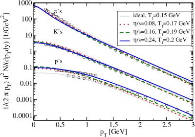
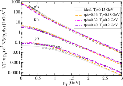
Figure 1: Viscous hydrodynamic fits of pion spectra to experimental data from PHENIX (circles) and STAR (squares) Adler:2003cb ; Adams:2003xp , for relaxation time values $\tau_{\Pi}=\frac{\eta}{s}\frac{6}{T}$ (left) and $\tau_{\Pi}=\frac{\eta}{s}\frac{1.5}{T}$ (right). Also shown are results for kaons and protons, scaled by $0.1$ and $0.01$, respectively. (The hydrodynamic results and the STAR data include weak decays while the PHENIX data does not). See text for details.

The initial central temperature $T_{0}$ and the freeze-out temperature $T_{f}$ are adjusted such that both the normalization and slope of the resulting pion spectrum is in reasonable agreement with experimental data Adler:2003cb ; Adams:2003xp . This is the procedure adopted in ideal hydrodynamics Huovinen:2006jp , and – as anticipated in Ref. Baier:2006um ; Baier:2006gy – can be carried through also for non-vanishing $\eta/s$, as is shown in Fig. 1. Usually, in addition the initialization time $\tau_{0}$ is allowed to vary in order to obtain a best fit also of the elliptic flow experimental data. Since in this work only central collisions are studied, the choice $\tau_{0}=1$ fm/c is adopted, but results should not depend strongly on this choice.

In Fig. 1, results for the spectra of pions, kaons and protons for various hydrodynamic runs with different values of shear viscosity are shown together with experimental data from PHENIX Adler:2003cb and STAR Adams:2003xp experiments for the most central $5$% of Au+Au collisions at $\sqrt{s_{NN}}=200$ GeV. It should be noted that no chemical potential is included in the equation of state, and therefore a distinction between particles and anti-particles is not possible. As a consequence, the spectrum of protons cannot be expected to match the experimental data, but is included in order to demonstrate that it is at least close to the experimental result.

In general, increasing the value of $\eta/s$ and leaving the initial and freeze-out conditions unchanged tends to make resulting spectra flatter Teaney ; Muronga:2004sf ; Chaudhuri:2005ea ; Baier:2006gy and hence in some sense mimics increasingly stronger transverse flow. Starting from initial/freeze-out conditions for which ideal hydrodynamics fits the experimental spectra and smoothly “turning on” viscosity, one has to counteract the effect of $\eta/s$ by reducing the buildup of transverse flow to keep the spectra in agreement with the experimental data. Both decreasing the initial central temperature and increasing the freeze-out temperature reduces the amount of hydrodynamic transverse flow at freeze-out. The former significantly affects the total pion multiplicity whereas the latter does not, offering a convenient way of decreasing total transverse flow while keeping the overall meson multiplicity close to data. However, since the concept of the Cooper-Frye freeze-out mechanism including the effects from resonance decays probably does not make sense at temperatures that are too high (far above $T_{c}\simeq 175$ MeV), an upper limit $T_{f}\leq 200$ MeV is imposed. This limiting $T_{f}$ is much larger than what is typically used in ideal hydrodynamic model fits. However, in ideal hydrodynamics the system interactions by definition always keep the system in perfect thermal equilibrium, while the presence of viscosity means that interactions are not as efficient, allowing for departures from equilibrium. As a consequence, an earlier freezing-out and thus a higher $T_{f}$ for viscous hydrodynamics as compared to ideal hydrodynamics is to be expected.

	$\frac{dN_{\pi,\rm visc}}{dy}/\frac{dN_{\pi,\rm ideal}}{dy}$	$\frac{dN_{K,\rm visc}}{dy}/\frac{dN_{K,\rm ideal}}{dy}$
$\eta/s=0.08$	1.06	1.06
$\eta/s=0.16$, $\tau_{\Pi}=\frac{\eta}{s}\frac{6}{T}$	1.12	1.12
$\eta/s=0.16$, $\tau_{\Pi}=\frac{\eta}{s}\frac{1.5}{T}$	1.12	1.12
$\eta/s=0.24$, $\tau_{\Pi}=\frac{\eta}{s}\frac{6}{T}$	1.15	1.15
$\eta/s=0.24$ $\tau_{\Pi}=\frac{\eta}{s}\frac{1.5}{T}$	1.18	1.19
$\eta/s=0.32$	1.23	1.23
$\eta/s=0.40$	1.28	1.28

Table 1: Fraction of multiplicity due to viscous entropy production: shown are the ratios of total multiplicities for pions and kaons calculated in viscous and ideal hydrodynamics, for identical initial/freeze-out conditions.

In Fig. 1, results are shown for a relaxation time value of $\tau_{\Pi}=\frac{\eta}{s}\frac{6}{T}$ (left) and $\tau_{\Pi}=\frac{\eta}{s}\frac{1.5}{T}$ (right) and various $\eta/s$. For $\tau_{\Pi}=\frac{\eta}{s}\frac{6}{T}$ the values of $T_{0}$ used to generate the figure are $T_{0}=0.34,0.33,0.33$ GeV for $\eta/s=0.08,0.16,0.24$. For $\tau_{\Pi}=\frac{\eta}{s}\frac{1.5}{T}$ the values are $T_{0}=0.34,0.32,0.31$ GeV for $\eta/s=0.16,0.32,0.40$. From this figure, it can be seen that for the larger value of $\tau_{\Pi}$, the pion (and kaon) spectra in viscous hydrodynamics can be made to agree reasonably well with experimental data up to $\eta/s\sim 0.25$ by mainly changing the freeze-out temperature $T_{f}$. At higher values of $\eta/s$, the pion spectrum becomes either too flat (when leaving $T_{0},T_{f}$ unchanged), the pion multiplicity becomes too low (when $T_{0}$ is lowered such that the slope matches the data) or one has to choose an unreasonably large $T_{f}>200$ MeV.

The same is true when adopting a smaller value of $\tau_{\Pi}$, but it is possible to have reasonable agreement with experimental data up to $\eta/s\sim 0.4$ (see Fig. 1), about twice the bound from the larger value of $\tau_{\Pi}$. A more detailed study of the effect of changing $\tau_{\Pi}$ is currently in progress prep .

For non-vanishing viscosity, the hydrodynamic evolution is no longer isentropic. Some part of the final multiplicity is therefore due to entropy production; in order to give some quantitative answers how much entropy is created, it is instructive to consider the ratio of meson multiplicities at non-vanishing $\eta/s$ and ideal hydrodynamics for identical initial/freeze-out conditions. Using the initial/freeze-out conditions for which the viscous calculations match the experimental pion spectrum, one finds the results shown in Table 1. It seems plausible to infer from Table 1 that final multiplicities are increased by a fraction of $\sim 0.75\,\eta/s$ with respect to ideal hydrodynamics due to viscous entropy production. Roughly, this translates to a percentage from $50\,\eta/s$ to $75\,\eta/s$ of the final multiplicity being due to viscous effects.

IV.2 HBT Radii

Using the definition of the HBT radii from the previous section and the initial/freeze-out conditions for which the viscous hydrodynamic calculation matches the experimental pion spectrum, one can proceed to compare the viscous hydrodynamic results for the HBT radii to experimental data. This is done in Fig. 2, where the ratios $R_{\rm out}/R_{\rm side}$ and $R_{\rm long}/R_{\rm side}$ for various values of $\eta/s$ are compared to data from STAR Adams:2004yc . The ratio $R_{\rm long}/R_{\rm out}$ is of special interest since in ideal hydrodynamics it has been notoriously hard to obtain results that are not far above the experimental data (which sometimes is known as the “HBT puzzle”). It has been argued in Refs. Dumitru:2002sq ; Teaney ; Muronga:2004sf that non-vanishing viscosity may decrease this ratio and thus bring it closer to the data. Fig. 2 represents the first result of the ratio $R_{\rm long}/R_{\rm out}$ for non-vanishing viscosity and initial/freeze-out conditions for which the experimental pion spectrum is matched at the same time.

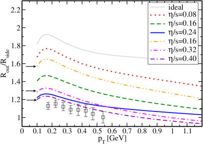
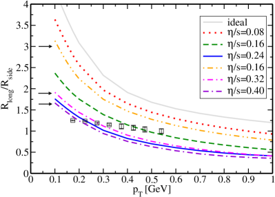
Figure 2: Pion HBT Radii from hydrodynamics compared to data from the STAR experiment Adams:2004yc . Shown are the ratios $R_{\rm out}/R_{\rm side}$ (left) and $R_{\rm long}/R_{\rm side}$ (right) for ideal and viscous hydrodynamics (with $\tau_{\Pi}=\frac{\eta}{s}\frac{6}{T}$ except for results indicated by arrows where $\tau_{\Pi}=\frac{\eta}{s}\frac{1.5}{T}$). See text for details.

As can be seen from this figure, the ratio $R_{\rm out}/R_{\rm side}$ approaches the experimental data as viscosity is increased. Indeed, for all but the lowest $p_{\perp}$ values the ratio is consistent with the data (within error bars) for the highest value of viscosity where the pion spectrum still matches the experimental data. Remarkable as this may be, it is unlikely that the presence of viscosity completely solves the HBT puzzle, the reason being that even though the ratio $R_{\rm out}/R_{\rm side}$ in the viscous hydrodynamic calculations moves close to data, the absolute values $R_{\rm out}$, $R_{\rm side}$ tend to be below the experimental values, as can be seen from Fig. 3. Put differently, the agreement of $R_{\rm out}/R_{\rm side}$ with data is achieved mainly by lowering $R_{\rm out}$, while $R_{\rm side}$ is hardly affected and always stays much below the experimental values.

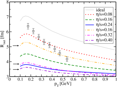
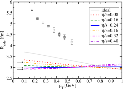
Figure 3: Pion HBT Radii from hydrodynamics compared to data from the STAR experiment Adams:2004yc . Shown are $R_{\rm out}$ (left) and $R_{\rm side}$ (right) for ideal and viscous hydrodynamics (with $\tau_{\Pi}=\frac{\eta}{s}\frac{6}{T}$ except for results indicated by arrows where $\tau_{\Pi}=\frac{\eta}{s}\frac{1.5}{T}$). See text for details.

At present, it is not excluded that a match of the viscous hydrodynamic $R_{\rm side}$ with experimental data can be achieved when e.g. when changing also the hydrodynamic initialization time $\tau_{0}$, or the initial energy density profile Huovinen:2006jp . However, the mismatch of $R_{\rm side}$ with data could also indicate that other effects, such as the replacement of the sharp hypersurface freeze-out by a more realistic continuous emission of particles Grassi:2000ke ; Sinyukov:2002if have to be taken into account to obtain a proper description of the experimental HBT radii.

Also shown in Fig. 2 is the ratio $R_{\rm long}/R_{\rm side}$, compared to experimental data Adams:2004yc . In this case, the viscous hydrodynamic result can be made to intersect the experimental results, but the too steep slope seems to prevent a nice match to data. Again the absolute values tend to be below the experimental data, also perhaps indicating the need for a more realistic freeze-out treatment.

V Conclusions

Using a simple numerical code to solve the causal viscous hydrodynamic equations for the case of central heavy-ion collisions, it has been shown that both pion total multiplicities and spectral slopes for Au+Au collisions at $\sqrt{s_{NN}}=200$ GeV can be matched to experimental data for moderate viscosities. The bound on $\eta/s$ up to which this matching is possible depends on the value of the relaxation time (which is a priori a free parameter of the causal viscous hydrodynamic framework) and on the hydrodynamic initialization time $\tau_{0}$. Setting $\tau_{0}=1$ fm/c, one obtains $\eta/s\lesssim 0.25$ for a value of the relaxation time $\tau_{\Pi}$ that corresponds to the weak-coupling QCD result, and $\eta/s\lesssim 0.4$ for a somewhat smaller value of $\tau_{\Pi}$. For all the viscous hydrodynamic calculations that result in a pion spectrum matching the experimental data, it was found that roughly $50\,\eta/s$ to $75\,\eta/s$ percent of the final multiplicity is due to viscous entropy production.

For hydrodynamic parameters that allow to match the experimental pion spectrum, it was shown that the ratio of HBT radii $R_{\rm out}/R_{\rm side}$ approaches and eventually matches the experimental result as $\eta/s$ is increased. The absolute values of $R_{\rm out}$, $R_{\rm side}$, however, tend to be much below the experimental values, suggesting that a more elaborate freeze-out treatment (or other effects, see e.g. Ref. Cramer:2004ih ) might be necessary to achieve agreement.

The above bound on the ratio $\eta/s\lesssim 0.4$ is interesting since it lies roughly half-way in between the weak-coupling QCD result Trans1 ; Trans2 and the strong coupling ${\mathcal{N}}=4$ SYM result Kovtun:2004de ; Janik:2006ft . If this bound was saturated, this could suggest that the quark-gluon plasma created at the highest RHIC energies is neither a very weakly nor a very strongly coupled plasma, but rather a border-case between these two. While this may not be the most elegant of possibilities that nature could have chosen, a not-weakly, not-strongly coupled plasma which behaves as a non-ideal fluid might be the most realistic assessment of the current status of RHIC data (see Ref. Romatschke:2006bb ; Huot:2006ys ; Blaizot:2006tk for related conclusions).

To decide, and maybe extract a value of the ratio $\eta/s$ (and at the same time $\tau_{\Pi}$) from RHIC data, it seems necessary to extend this work to the treatment of non-central collisions, and thus viscous hydrodynamic results for elliptic flow.

- (1) W.A. Hiscock and L. Lindblom, Phys. Rev. D 31, 725 (1985).
- (2) W. Israel, Ann.Phys. 100 (1976) 310; W. Israel and J.M. Stewart, Phys. Lett. 58A (1976) 213; W. Israel and J.M. Stewart, Ann.Phys. 118, (1979) 341.
- (3) I-Shih Liu, I. Müller and T. Ruggeri, Ann.Phys. 169 (1986) 191.
- (4) A. Muronga, Phys. Rev. Lett. 88 (2002) 062302 [Erratum-ibid. 89 (2002) 159901].
- (5) A. Muronga, Phys. Rev. C 69 (2004) 034903.
- (6) R. Baier, P. Romatschke and U. A. Wiedemann, Phys. Rev. C 73 (2006) 064903.
- (7) T. Koide, G. S. Denicol, Ph. Mota and T. Kodama, arXiv:hep-ph/0609117.
- (8) A. Muronga and D. H. Rischke, arXiv:nucl-th/0407114.
- (9) A. K. Chaudhuri and U. W. Heinz, J. Phys. Conf. Ser. 50 (2006) 251.
- (10) R. Baier and P. Romatschke, arXiv:nucl-th/0610108.
- (11) P. Arnold, G. D. Moore and L. G. Yaffe, JHEP 0011 (2000) 001.
- (12) P. Arnold, G. D. Moore and L. G. Yaffe, JHEP 0305 (2003) 051.
- (13) P. Kovtun, D. T. Son and A. O. Starinets, Phys. Rev. Lett. 94 (2005) 111601.
- (14) R. A. Janik, Phys. Rev. Lett. 98 (2007) 022302.
- (15) M. Asakawa, S. A. Bass and B. Muller, Phys. Rev. Lett. 96 (2006) 252301.
- (16) S. Mrowczynski, Acta Phys. Polon. B 37 (2006) 427.
- (17) P. Arnold, C. Dogan and G. D. Moore, Phys. Rev. D 74 (2006) 085021.
- (18) U. W. Heinz, H. Song and A. K. Chaudhuri, Phys. Rev. C 73 (2006) 034904.
- (19) A. Muronga, arXiv:nucl-th/0611090.
- (20) R. Baier, P. Romatschke and A. Starinets, in preparation.
- (21) P. F. Kolb, U. W. Heinz, P. Huovinen, K. J. Eskola and K. Tuominen, Nucl. Phys. A 696 (2001) 197.
- (22) Y. Aoki, Z. Fodor, G. Endrodi, S.D. Katz and K.K. Szabo, Nature 443 (2006) 675.
- (23) M. Laine and Y. Schroder, Phys. Rev. D 73 (2006) 085009.
- (24) F. Cooper and G. Frye, Phys. Rev. D 10, 186 (1974).
- (25) D. H. Rischke and M. Gyulassy, Nucl. Phys. A 608 (1996) 479.
- (26) D. Teaney, Phys. Rev. C 68 (2003) 034913.
- (27) B. R. Schlei, U. Ornik, M. Plumer and R. M. Weiner, Phys. Lett. B 293 (1992) 275.
- (28) S. Pratt, Phys. Rev. D 33 (1986) 72.
- (29) G. F. Bertsch, Nucl. Phys. A 498 (1989) 173C.
- (30) Version 0.2, available from http://nt3.phys.columbia.edu/people/molnard/OSCAR/
- (31) J. Sollfrank, P. Koch and U. W. Heinz, Phys. Lett. B 252 (1990) 256.
- (32) J. Sollfrank, P. Koch and U. W. Heinz, Z. Phys. C 52 (1991) 593.
- (33) S. S. Adler et al. [PHENIX Collaboration], Phys. Rev. C 69 (2004) 034909.
- (34) J. Adams et al. [STAR Collaboration], Phys. Rev. Lett. 92 (2004) 112301.
- (35) P. Huovinen and P. V. Ruuskanen, arXiv:nucl-th/0605008.
- (36) J. Adams et al. [STAR Collaboration], Phys. Rev. C 71 (2005) 044906.
- (37) A. Dumitru, arXiv:nucl-th/0206011.
- (38) F. Grassi, Y. Hama, S. S. Padula and O. J. Socolowski, Phys. Rev. C 62 (2000) 044904.
- (39) Yu. M. Sinyukov, S. V. Akkelin and Y. Hama, Phys. Rev. Lett. 89 (2002) 052301.
- (40) J. G. Cramer, G. A. Miller, J. M. S. Wu and J. H. S. Yoon, Phys. Rev. Lett. 94 (2005) 102302.
- (41) P. Romatschke, Phys. Rev. C 75, (2007) 014901.
- (42) S. C. Huot, S. Jeon and G. D. Moore, arXiv:hep-ph/0608062.
- (43) J. P. Blaizot, E. Iancu, U. Kraemmer and A. Rebhan, arXiv:hep-ph/0611393.