Superscaling in electroweak excitation of nuclei

Abstract

Superscaling properties of ¹²C , ¹⁶O and ⁴⁰Ca nuclear responses, induced by electron and neutrino scattering, are studied for momentum transfer values between 300 and 700 MeV/$c$. We have defined two indexes to have quantitative estimates of the scaling quality. We have analyzed experimental responses to get the empirical values of the two indexes. We have then investigated the effects of finite dimensions, collective excitations, meson exchange currents, short-range correlations and final state interactions. These effects strongly modify the relativistic Fermi gas scaling functions, but they conserve the scaling properties. We used the scaling functions to predict electron and neutrino cross sections and we tested their validity by comparing them with the cross sections obtained with a full calculation. For electron scattering we also made a comparison with data. We have calculated the total charge-exchange neutrino cross sections for neutrino energies up to 300 MeV.

I INTRODUCTION

The properties of the Relativistic Fermi Gas (RFG) model of the nucleus Alberico et al. (1988); DePace (1998); Amaro et al. (2002) have inspired the idea of superscaling. In the RFG model, the responses of the system to an external perturbation are related to a universal function of a properly defined scaling variable which depends on the energy and the momentum transferred to the system. With the adjective universal we want to indicate that the scaling function is independent of the momentum transfer, and also of the number of nucleons. These properties are respectively called scaling of first and second kind. Furthermore, the scaling function can be defined in such a way to result in independence also of the specific type of external one-body operator. This feature is usually called scaling of zeroth kind Maieron et al. (2002); Amaro et al. (2005a, b). One has superscaling when the three kinds of scaling we have described are verified. This happens in the RFG model.

The theoretical hypothesis of superscaling can be empirically tested by extracting response functions from the experimental cross sections and by studying their scaling behaviours. The responses of the nucleus to electroweak probes can be extracted from the lepton-nucleus cross sections by dividing them by the single-nucleon cross sections properly weighted to account for the number of protons and neutrons. In addition, one has to divide the obtained responses by the appropriate electroweak form factors.

Inclusive electron scattering data in the quasi-elastic region have been analyzed in this way Donnelly and Sick (1999a, b); Maieron et al. (2002). The main result of these studies is that the longitudinal responses show superscaling behaviour. To be more specific, scaling of second kind, independence of the nucleus, is better fulfilled than the scaling of first kind, independence of the momentum transfer. The situation for the transverse responses is much more complicated.

The presence of superscaling features in the data is relevant not only by itself, but mainly because this property can be used to make predictions. In effect, from a specific set of longitudinal response data Jourdan (1996), an empirical universal scaling function has been extracted Maieron et al. (2002) and has been used to obtain neutrino-nucleus cross sections in the quasi-elastic region Amaro et al. (2005a).

We observed that this universal scaling function is quite different from that predicted by the RFG model. This indicates the presence of physical effects not included in the RFG model, but still conserving the scaling properties. We have investigated the superscaling behaviour of some of the effects not considered in the RFG model. They are: the finite size of the system, its collective excitations, the Short-Range Correlations (SRC), the Meson Exchange Currents (MEC) and the Final State Interactions (FSI). The inclusion of these effects produce scaling functions rather similar to the empirical ones.

Before presenting our results, we recall in Sec. II the basic expressions of the superscaling formalism. We show how the scaling functions are related to the electromagnetic and weak response functions, and to the inclusive lepton scattering cross sections.

In Sec. III we discuss the scaling properties of our nuclear models. To quantify the quality of the scaling between the various functions obtained with different calculations, we define two indexes, ${\cal R}$ and ${\cal D}$. From the data of Ref. Jourdan (1996) we extract empirical reference values of these two indexes which indicate if scaling has occurred. From the same set of data we also extract an empirical universal scaling function. We analyze the scaling properties of all the effects beyond the RFG model, by comparing the values of the two indexes ${\cal R}$ and ${\cal D}$ of the theoretical scaling functions with the empirical ones. We choose a theoretical scaling function obtained by including all the effects considered as a theoretical universal scaling function.

In Sec. IV we study the prediction power of the superscaling hypothesis. Our universal empirical and theoretical scaling functions are used to calculate electron and neutrino inclusive cross sections. These results are compared with those obtained by calculating the same cross sections with our nuclear model. We discuss results for double differential electron scattering processes, and compare our cross sections with experimental data. We calculate also total neutrino cross sections for neutrino energies up to 300 MeV. In Sec. V we summarize our results and present our conclusions.

II BASIC SCALING FORMALISM

Scaling variables and functions have been presented in a number of papers Alberico et al. (1988); Barbaro et al. (1998); Donnelly and Sick (1999a, b); Maieron et al. (2002); Barbaro et al. (2004); Amaro et al. (2005a, b, 2006); Antonov et al. (2006). The purpose of this section is to recall the expression of the scaling variable used in our study and the relations between scaling functions, responses and cross sections.

In this work we have considered only processes of inclusive lepton scattering off nuclei. We have described these processes in Plane Wave Born Approximation and we have neglected the terms related to the rest masses of the leptons. In this presentation we indicate respectively with $\omega$ and ${\bf q}$ the energy and the momentum transferred to the nucleus.

In the RFG model the scaling variables and functions are related to the two free parameters of the model: the Fermi momentum $k_{\rm F}$ and the energy shift $E_{\rm shift}$. We define the quantity:

$$\Psi_{0}=\frac{2m}{k_{\rm F}}\left[\sqrt{\left(\frac{\omega-E_{\rm shift}}{2m}\right)\left(1+\frac{\omega-E_{\rm shift}}{2m}\right)}-\frac{q}{2m}\right]\,,$$ (1)

where $q\equiv|{\bf q}|$, and $m=(m_{p}+m_{n})/2$ indicates the average nucleon mass. The scaling variable is then defined as:

$$\Psi=\Psi_{0}\left(1+\Psi_{0}\frac{k_{\rm F}}{2q}\sqrt{\frac{q^{2}}{m^{2}}+1}\,\right)\,.$$ (2)

The RFG model provides a universal scaling function which can be expressed in terms of the scaling variable $\Psi$ as Amaro et al. (2005a, b):

$$f^{\rm RFG}(\Psi)=\frac{3}{4}\left(1-\Psi^{2}\right)\theta\left(1-\Psi^{2}\right)\,,$$ (3)

where $\theta(x)$ indicates the step function. The RFG scaling function (3) is normalized to unity.

In the electron scattering case, the inclusive double differential cross section can be written as Boffi et al. (1996):

$$\frac{{\rm d}^{2}\sigma}{{\rm d}\theta\,{\rm d}\omega}=\sigma_{\rm M}\left\{\frac{(\omega^{2}-q^{2})^{2}}{q^{4}}R_{\rm L}(\omega,q)+\left[\tan^{2}\left(\frac{\theta}{2}\right)-\frac{\omega^{2}-q^{2}}{2q^{2}}\right]R_{\rm T}(\omega,q)\right\}\,,$$ (4)

where $\theta$ is the scattering angle, $\sigma_{\rm M}$ is the Mott cross section, and we have indicated with $R_{\rm L}$ and $R_{\rm T}$ the longitudinal and transverse responses, respectively defined as:

$$R_{\rm L}(\omega,q)=4\pi\sum_{J=0}~{}|\langle J_{\rm f}||\mathcal{C}_{J}||J_{\rm i}\rangle|^{2}\,,$$ (5)

and

$$R_{\rm T}(\omega,q)=4\pi\sum_{J=1}~{}(|\langle J_{\rm f}||\mathcal{E}_{J}||J_{\rm i}\rangle|^{2}+|\langle J_{\rm f}||\mathcal{M}_{J}||J_{\rm i}\rangle|^{2})\,.$$ (6)

In the above equations we have indicated with $|J_{\rm i}\rangle$ and $|J_{\rm f}\rangle$ the initial and final states of the nucleus characterized by their total angular momenta $J_{\rm i}$ and $J_{\rm f}$. The double bars indicate that the angular momentum matrix elements are evaluated in their reduced expressions, as given by the Wigner-Eckart theorem Edmonds (1957). We have indicated with $\mathcal{C}_{J}$, $\mathcal{E}_{J}$ and $\mathcal{M}_{J}$ respectively the Coulomb, electric and magnetic multipole operators Boffi et al. (1996); Blatt and Weisskopf (1952).

The scaling functions are obtained from the electromagnetic responses as:

$$f_{\rm L}(\Psi) = k_{\rm F}\,\frac{q^{2}-\omega^{2}}{q\,m}\,\frac{R_{\rm L}(\omega,q)}{Z(G^{p}_{\rm E})^{2}+N(G^{n}_{\rm E})^{2}}\,,$$ (7)

$$f_{\rm T}(\Psi) = 2\,k_{\rm F}\,\frac{q\,m}{q^{2}-\omega^{2}}\,\frac{R_{\rm T}(\omega,q)}{Z(G^{p}_{\rm M})^{2}+N(G^{n}_{\rm M})^{2}}\,,$$ (8)

where $Z$ and $N$ indicate, respectively, the number of protons and neutrons of the target nucleus, and we have indicated with $G_{\rm E,M}^{p,n}$ the electric (E) and magnetic (M) form factors of the proton ($p$) and the neutron ($n$). In our calculations we used the electromagnetic nucleon form factors of Ref. Hoeler et al. (1976). In Eq. (8) only the magnetic nucleon form factors are present. This implies the hypothesis that in $R_{\rm T}$ only the one-body magnetization current is active. In the range of momentum transfer values investigated, from 300 to 700 MeV/$c$, we found that the contribution of the convection current is of few percents that of the magnetization current.

Since our calculations are done in a non relativistic framework, we have modified our responses by using the semi-relativistic corrections proposed in Amaro et al. (2005b, 1996):

$$\epsilon \rightarrow \epsilon\left(1+\frac{\epsilon}{2m}\right)\,,$$ (9)

$$R_{\rm L}(q,\omega) \rightarrow \frac{q^{2}}{q^{2}-\omega^{2}}\,R_{\rm L}(q,\omega)\,,$$ (10)

$$R_{\rm T}(q,\omega) \rightarrow \frac{q^{2}-\omega^{2}}{q^{2}}\,R_{\rm T}(q,\omega)\,,$$ (11)

where $\epsilon$ indicates the energy of the emitted nucleon.

The above discussion can be extended to the case of the inclusive neutrino scattering processes. For example, for the $(\nu_{e},e^{-})$ reaction we express the differential cross section as O’Connell et al. (1972); Walecka (1975, p. 113, 1995):

$$\frac{{\rm d}^{2}\sigma}{{\rm d}\Omega{\rm d}\omega} = \frac{G^{2}\cos^{2}\theta_{\rm C}}{(2\pi)^{2}}|\,{\bf k}_{\rm f}|\,\epsilon_{\rm f}\,F(Z^{\prime},\epsilon_{\rm f})\left\{\left(l_{0}l_{0}^{\star}+\frac{\omega^{2}}{q^{2}}l_{3}l_{3}^{\star}-\frac{\omega}{q}l_{3}l_{0}^{\star}\right)\,R_{\rm CC}^{\rm V}(\omega,q)\right.$$ (12)

$$+\,l_{0}l_{0}^{\star}\,R_{\rm CC}^{\rm A}(\omega,q)\,+\,l_{3}l_{3}^{\star}\,R_{\rm LL}^{\rm A}(\omega,q)\,+\,2\,l_{3}l_{0}^{\star}\,R_{\rm CL}^{\rm A}(\omega,q)$$

$$+\,\left.\frac{1}{2}\,\left(\vec{l}\cdot\vec{l}^{\star}-l_{3}l_{3}^{\star}\right)\,\left[R_{\rm T}^{\rm V}(\omega,q)+R_{\rm T}^{\rm A}(\omega,q)\right]\,-\,\frac{i}{2}\,\left(\vec{l}\times\vec{l}^{\star}\right)_{3}\,R^{VA}_{\rm T^{\prime}}(\omega,q)\right\}\,.$$

In the above equation we have indicated with $G$ the Fermi constant, with $\theta_{\rm C}$ the Cabibbo angle, with $\epsilon_{\rm f}$ and ${\bf k}_{\rm f}$ the energy and the momentum of the scattered lepton and with $F(Z^{\prime},\epsilon_{\rm f})$ the Fermi function taking into account the distortion of the electron wave function due to the Coulomb field of the daughter nucleus of charge $Z^{\prime}$. The expressions of the factors $l_{i}l_{i}^{\star}$, related only to the leptons variables, are given in Refs. O’Connell et al. (1972); Walecka (1975, p. 113, 1995).

The nuclear response functions are expressed in terms of multipole expansion of the operators describing the various terms of the weak interaction. They are the Coulomb $\mathcal{C}_{J}$, longitudinal $\mathcal{L}_{J}$, transverse electric $\mathcal{E}_{J}$ and transverse magnetic $\mathcal{M}_{J}$ operators. The responses are defined as:

$$R_{\rm CC}^{\rm V}(\omega,q)=4\pi\sum_{J=0}~{}|\langle J_{\rm f}||\mathcal{C}_{J}^{\rm V}||J_{\rm i}\rangle|^{2}\,,$$ (13)

$$R_{\rm CC}^{\rm A}(\omega,q)=4\pi\sum_{J=0}~{}|\langle J_{\rm f}||\mathcal{C}_{J}^{\rm A}||J_{\rm i}\rangle|^{2}\,,$$ (14)

$$R_{\rm CL}^{\rm A}(\omega,q)=2\pi~{}\sum_{J=0}\left(\langle J_{\rm f}||\mathcal{C}_{J}^{\rm A}||J_{\rm i}\rangle^{\star}\langle J_{\rm f}||\mathcal{L}_{J}^{\rm A}||J_{\rm i}\rangle+\langle J_{\rm f}||\mathcal{C}_{J}^{\rm A}||J_{\rm i}\rangle\langle J_{\rm f}||\mathcal{L}_{J}^{\rm A}||J_{\rm i}\rangle^{\star}\right)\,,$$ (15)

$$R_{\rm LL}^{\rm A}(\omega,q)=4\pi\sum_{J=0}~{}|\langle J_{\rm f}||\mathcal{L}_{J}^{\rm A}||J_{\rm i}\rangle|^{2}\,,$$ (16)

$$R_{\rm T}^{\rm V}(\omega,q)=4\pi\sum_{J=1}\,\left(|\langle J_{\rm f}||\mathcal{E}_{J}^{\rm V}||J_{\rm i}\rangle|^{2}+|\langle J_{\rm f}||\mathcal{M}_{J}^{\rm V}||J_{\rm i}\rangle|^{2}\right)\,,$$ (17)

$$R_{\rm T}^{\rm A}(\omega,q)=4\pi\sum_{J=1}\,\left(|\langle J_{\rm f}||\mathcal{E}_{J}^{\rm A}||J_{\rm i}\rangle|^{2}+|\langle J_{\rm f}||\mathcal{M}_{J}^{\rm A}||J_{\rm i}\rangle|^{2}\right)\,,$$ (18)

and

$$R_{\rm T^{\prime}}^{\rm VA}(\omega,q)=2\pi~{}\sum_{J=1} \left(\langle J_{\rm f}||\mathcal{E}_{J}^{\rm V}||J_{\rm i}\rangle^{\star}\langle J_{\rm f}||\mathcal{M}_{J}^{\rm A}||J_{\rm i}\rangle+\langle J_{\rm f}||\mathcal{E}_{J}^{\rm V}||J_{\rm i}\rangle\langle J_{\rm f}||\mathcal{M}_{J}^{\rm A}||J_{\rm i}\rangle^{\star}+\right.$$ (19)

$$\left.\langle J_{\rm f}||\mathcal{E}_{J}^{\rm A}||J_{\rm i}\rangle^{\star}\langle J_{\rm f}||\mathcal{M}_{J}^{\rm V}||J_{\rm i}\rangle+\langle J_{\rm f}||\mathcal{E}_{J}^{\rm A}||J_{\rm i}\rangle\langle J_{\rm f}||\mathcal{M}_{J}^{\rm V}||J_{\rm i}\rangle^{\star}\right)\,,$$

where we have separated the vector (V) and the axial-vector (A) contributions.

We found that the terms related to the axial-Coulomb operator $\mathcal{C}^{\rm A}_{J}$ give a very small contribution to the cross section, and, in our study, we neglected them. This means that our scaling analysis has been done for the $R_{\rm CC}^{\rm V}$, $R_{\rm LL}^{\rm A}$, $R_{\rm T}^{\rm V}$, $R_{\rm T}^{\rm A}$ and $R_{\rm T^{\prime}}^{\rm VA}$ responses only. The corresponding scaling functions have been defined as:

$$f_{\rm CC}^{\rm V}(\Psi) = k_{\rm F}\,\frac{q^{2}-\omega^{2}}{q\,m}\,\frac{R_{\rm CC}^{\rm V}(\omega,q)}{N(G^{(1)}_{\rm E})^{2}}\,,$$ (20)

$$f_{\rm LL}^{\rm A}(\Psi) = 4\,k_{\rm F}\,\frac{q\,m}{4m^{2}+q^{2}-\omega^{2}}\,\frac{R_{\rm LL}^{\rm A}(\omega,q)}{N(G_{\rm A})^{2}}\,,$$ (21)

$$f_{\rm T}^{\rm V}(\Psi) = 2\,k_{\rm F}\,\frac{q\,m}{q^{2}-\omega^{2}}\,\frac{R_{\rm T}^{\rm V}(\omega,q)}{N(G^{(1)}_{\rm M})^{2}}\,,$$ (22)

$$f_{\rm T}^{\rm A}(\Psi) = 2\,k_{\rm F}\,\frac{q\,m}{4m^{2}+q^{2}-\omega^{2}}\,\frac{R_{\rm T}^{\rm A}(\omega,q)}{N(G_{\rm A})^{2}}\,,$$ (23)

$$f_{\rm T^{\prime}}^{\rm VA}(\Psi) = 2\,k_{\rm F}\,\frac{q\,m}{\sqrt{q^{2}-\omega^{2}}\sqrt{4m^{2}+q^{2}-\omega^{2}}}\,\frac{R_{\rm T^{\prime}}^{\rm VA}(\omega,q)}{NG^{(1)}_{\rm M}G_{\rm A}}\,,$$ (24)

where we have indicated with $G^{(1)}_{\rm E,M}$ the isovector electric (E) and magnetic (M) nucleon form factors, and with $G_{\rm A}$ the axial-vector one. We have used the electromagnetic form factors of Ref. Hoeler et al. (1976), and the dipole form of the axial vector form factor with an axial mass value of 1030 MeV.

The relativistic effects are taken into account by using semi-relativistic corrections similar to those of Eqs. (9)-(11). In this case the responses are obtained by doing the following changes with respect to the pure non relativistic case:

$$R_{\rm CC}^{\rm V}(q,\omega) \rightarrow \frac{q^{2}}{q^{2}-\omega^{2}}\,R_{\rm CC}^{\rm V}(q,\omega)\,,$$ (25)

$$R_{\rm LL}^{\rm A}(q,\omega) \rightarrow \left(1+\frac{q^{2}-\omega^{2}}{4m^{2}}\right)\,R_{\rm LL}^{\rm A}(q,\omega)\,,$$ (26)

$$R_{\rm T}^{\rm V}(q,\omega) \rightarrow \frac{q^{2}-\omega^{2}}{q^{2}}\,R_{\rm T}^{\rm V}(q,\omega)\,,$$ (27)

$$R_{\rm T}^{\rm A}(q,\omega) \rightarrow \left(1+\frac{q^{2}-\omega^{2}}{4m^{2}}\right)\,R_{\rm T}^{\rm A}(q,\omega)\,,$$ (28)

$$R_{\rm T^{\prime}}^{\rm VA}(q,\omega) \rightarrow \sqrt{\frac{q^{2}-\omega^{2}}{q^{2}}}\,\sqrt{1+\frac{q^{2}-\omega^{2}}{4m^{2}}}\,R_{\rm T^{\prime}}^{\rm VA}(q,\omega)\,.$$ (29)

The extension of these expressions to antineutrino charge exchange scattering processes is straightforward. The treatment of charge conserving processes is slightly different.

III SUPERSCALING BEYOND RFG MODEL

The basic quantities calculated in our work are the electromagnetic, and the weak, nuclear response functions. We obtain the scaling functions by using Eqs. (7) and (8) for the electron scattering case, and Eqs. (20)-(24) for the neutrino scattering. The scaling properties of the scaling functions have been studied by a direct numerical comparison. We thought it necessary to define some numerical index able to quantify the quality of the scaling.

Let us consider the problem of comparing a number $M$ of scaling functions $\left\{{f_{\alpha},\alpha=1,\ldots,M}\right\}$, each of them known for $K$ values of the scaling variable $\left\{\Psi_{i},i=1,\ldots,K\right\}$. For each value of $\Psi_{i}$ we found the maximum and minimum of the various $f_{\alpha}$ scaling functions:

$$f^{\rm max}_{i}\,=\,\max_{\alpha=1,\ldots,M}\left[f_{\alpha}(\Psi_{i})\right]\,,$$ (30)

$$f^{\rm min}_{i}\,=\,\min_{\alpha=1,\ldots,M}\left[f_{\alpha}(\Psi_{i})\right]\,.$$ (31)

We define the two indexes

$${\cal D}\,=\,\max_{i=1,\ldots,K}\left[f^{\rm max}_{i}\,-\,f^{\rm min}_{i}\right]\,,$$ (32)

and

$${\cal R}=\frac{1}{Kf^{\max}}\sum_{i=1,\ldots,K}\left[f^{\rm max}_{i}-f^{\rm min}_{i}\right]\,,$$ (33)

where $f^{\rm max}$ is:

$$f^{\rm max}\,=\,\max_{i=1,\ldots,K}\left[f^{\rm max}_{i}\right]\,.$$ (34)

The two indexes give complementary information. The ${\cal D}$ index is related to a local property of the functions: the maximum distance between the various curves. The value of this index could be misleading if the responses have sharp resonances. For this reason we have also used the ${\cal R}$ index which is instead sensitive to global properties of the differences between the functions. Since we know that the functions we want to compare are roughly bell shaped, we have inserted the factor $1/f^{\rm max}$ to weight more the region of the maxima of the functions than that of the tails.

The perfect scaling is obtained when both ${\cal D}$ and ${\cal R}$ are zero. This is achieved only in the RFG model. In our calculations the perfect scaling is obviously violated, as it is violated by the empirical scaling functions. In order to have reference values of the two indexes we have determined the values of ${\cal R}$ and ${\cal D}$ for experimental scaling functions extracted from the longitudinal and transverse electromagnetic response data of ¹²C, ⁴⁰Ca and ⁵⁶Fe given in Ref. Jourdan (1996). This is the same set of data used in Ref. Maieron et al. (2002) to extract a universal scaling function.

The definition of the scaling variable $\Psi$, Eqs. (1) and (2), requires on to fix the values of $k_{\rm F}$ and $E_{\rm shift}$ for each nucleus. We used values of $k_{\rm F}$ obtained by doing an average over the nuclear density, and values of $E_{\rm shift}$ that, in a Fermi gas calculation, reproduce the peak position of the experimental response functions Amaro et al. (1994a). We used $E_{\rm shift}$=15 MeV for all the nuclei and $k_{\rm F}$=215 MeV/$c$ for ¹²C and ¹⁶O and $k_{\rm F}$=245 MeV/$c$ for ⁴⁰Ca and ⁵⁶Fe.

	$f_{\rm L}$		$f_{\rm T}$
$q$ [MeV/$c$]	${\cal D}$	${\cal R}$	${\cal D}$	${\cal R}$
300	0.107 $\pm$ 0.002	0.152 $\pm$ 0.013	0.223 $\pm$ 0.004	0.165 $\pm$ 0.017
380	0.079 $\pm$ 0.003	0.075 $\pm$ 0.009	0.235 $\pm$ 0.005	0.155 $\pm$ 0.014
570	0.101 $\pm$ 0.009	0.079 $\pm$ 0.017	0.169 $\pm$ 0.003	0.082 $\pm$ 0.007

Table 1: Values of the ${\cal D}$ and ${\cal R}$ indexes, Eqs. (32) and (33), calculated by comparing the empirical $f_{\rm L}$ and $f_{\rm T}$ scaling functions shown in Fig. 1 for each value of the momentum transfer $q$. The values provide information about the scaling of second kind. The values of the ${\cal D}$ and ${\cal R}$ for $f_{\rm L}$ at $q$=570 MeV/$c$, in boldface, are taken as our reference values.

The details of the procedures we have used to extract the experimental scaling functions and to calculate the empirical values of ${\cal R}$ and ${\cal D}$ are given in Appendix A. We present in Fig. 1 the experimental longitudinal and transverse scaling function data for ¹²C, ⁴⁰Ca and ⁵⁶Fe for each value of the momentum transfer given in Ref. Jourdan (1996). In Table 1 we give the values of ${\cal D}$ and ${\cal R}$ obtained by comparing the experimental scaling functions shown in each panel.

We analyze the empirical scaling functions by studying the three different kinds of scaling defined in the Introduction. The presentation of the data of Fig. 1 and Table 1 gives direct information on the scaling of second kind. It is immediate to observe that, in this case, the $f_{\rm L}$ functions scale better than the $f_{\rm T}$ ones. The $f_{\rm T}$ scaling functions of ¹²C, especially for the lower $q$ values, are remarkably different from those of ⁴⁰Ca and ⁵⁶Fe. This is confirmed by the values of ${\cal R}$ and ${\cal D}$ given in Table 1.

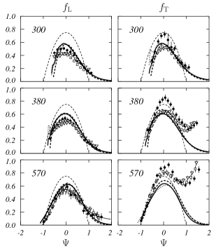
Figure 1: Empirical longitudinal, $f_{\rm L}$, and transverse, $f_{\rm T}$, scaling functions obtained from the experimental electromagnetic responses of Ref. Jourdan (1996) as explained in Appendix A. The numbers in the panels indicate the values of the momentum transfer in MeV/$c$. The full circles refer to ¹²C, the white squares to ⁴⁰Ca, and the white triangles to ⁵⁶Fe. The thin black line in the $f_{\rm L}$ panel at 570 MeV/$c$, is the empirical scaling function obtained by fitting the data. The thick lines show the results of our calculations when all the effects beyond the RFG model have been considered (see text). The full lines have been calculated for ¹²C, the dotted lines for ¹⁶O, and the dashed lines for ⁴⁰Ca. The thin dashed lines show the RFG scaling functions.

The other two kinds of scaling are not so well fulfilled by the experimental functions. It is evident, from the figure, the poor quality of the scaling of zeroth kind. Longitudinal and transverse scaling functions are remarkably different, not only in size, but even in their shapes. The excitation of subnucleonic degrees of freedom, mainly the excitation of the $\Delta$ resonance, strongly affects $f_{\rm T}$, while it is almost irrelevant in $f_{\rm L}$. Also the quality of the scaling of first kind is rather poor. These observations are in agreement with those of Refs. Donnelly and Sick (1999a, b); Maieron et al. (2002) where also data measured at large $q$ values have been used.

From the analysis of the scaling properties of the experimental functions, we have extracted two benchmark values of ${\cal R}$ and ${\cal D}$ that we have used to gauge the quality of the scaling of our theoretical functions. The values we have chosen are those related to the $f_{L}$ functions at $q$=570 MeV/c, see Tab. 1, where the quasi-elastic scattering mechanism works better. In the following, we shall consider that the scaling is violated when ${\cal R}>$0.096 or ${\cal D}>$ 0.11. These numbers are obtained by adding the uncertainty to the central benchmark values. The non scaling regions will be indicated by the gray areas in the figures.

From the same set of data we extracted, see Appendix A, an empirical universal scaling function represented by the thin full line in the lowest left panel of Fig. 1. This function, which we called $f_{\rm U}^{\rm ex}$, is rather similar to the universal empirical function given in Ref. Maieron et al. (2002).

We start now to consider the scaling of the theoretical functions. The thick lines show the results of our calculations when various effects beyond the RFG are introduced. These scaling functions have been obtained by considering the nuclear finite size, the collective excitations, the short-range correlations, the final state interactions, and, in the case of the $f_{\rm T}$ functions, the meson-exchange currents.

The results presented by the thick lines have been obtained for three different nuclei. The full lines represent the ¹²C results, while the dotted and dashed lines show, respectively, the results obtained for ¹⁶O and ⁴⁰Ca. The differences between these curves become larger with decreasing $q$ values. We obtain ${\cal R}$=0.03 and ${\cal D}$=0.05 for $f_{\rm L}$ at 570 MeV/$c$ and ${\cal R}$=0.05 and ${\cal D}$=0.15 at 300 MeV/$c$. The scaling of the $f_{\rm T}$ functions is not as good. In this case we obtain ${\cal R}$=0.03 and ${\cal D}$=0.06 at 570 MeV/$c$ and ${\cal R}$=0.10 and ${\cal D}$=0.13 at 300 MeV/$c$. In any case, these numbers are smaller than our empirical reference values, and we can state that the scaling of second kind is satisfied.

On the contrary, the curves of Fig. 1 show a poor scaling of first kind. The comparison between the $f_{\rm L}$ functions calculated for the three $q$ values indicated in the figure, gives a minimum ${\cal R}$ value of 0.13, found for ¹²C nucleus, and a maximum value of 0.15, found for the ⁴⁰Ca nucleus. The minimum and maximum values of the other index, ${\cal D}$, are 0.18 and 0.30. We found similar, even if few percents larger, values also for the $f_{\rm T}$ functions.

The scaling of zeroth kind is rather well satisfied. By comparing the $f_{\rm L}$ and $f_{\rm T}$ for each nucleus and each $q$ value we found 0.04 as a maximum value of ${\cal R}$. We found 0.11 for ${\cal D}$, slightly large even if below our empirical limiting value. This relatively large value of ${\cal D}$ is due to the presence of sharp resonances in the longitudinal and transverse responses at $q$=300 MeV/$c$ which appear at different excitation energies. We have chosen the longitudinal scaling function obtained for ¹⁶O at $q=570$ MeV/$c$ as the theoretical universal scaling function that we called $f_{\rm U}^{\rm th}$.

In Fig. 1 the thin dashed lines show the RFG scaling functions. It is evident that the inclusion of the effects beyond the RFG we have considered, produce relevant modifications of the RFG scaling functions. These modifications remarkably improve the agreement with the experimental scaling functions. On the other hand, the effects we have considered do not heavily modify the scaling properties of the $f_{\rm L}$ and $f_{\rm T}$ functions. In the remaining part of the section, we first discuss the consequences of each effect beyond RFG, and then we analyze the scaling properties for neutrino scattering processes.

III.1 Finite size effects

The starting point of our calculations is the continuum shell model. In this model, the scattering processes are described by using some assumption on the nuclear structure which are also used in the Fermi gas model. We refer to the fact that both nuclear models consider the nucleons free to move in a mean-field potential. The continuum shell model takes into account the finite dimensions of the system, the finite number of nucleons, and the fact that protons and neutrons feel different mean-field potentials. In our calculations, the mean-field is produced by a Woods-Saxon well. The parameters of this potential are taken from Refs. Botrugno and Co’ (2005) (for ¹²C) and de Saavedra et al. (1996) (for ¹⁶O and ⁴⁰Ca) and have been fixed to reproduce the single particle energies around the Fermi surface and the rms radii of the charge distributions of each nucleus we have considered.

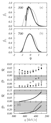
Figure 2: Continuum shell model results. In the panels (a) and (b), the thick lines represent the $f_{\rm L}$ scaling functions calculated for the various nuclei: full lines ¹²C, dotted lines ¹⁶O, dashed lines ⁴⁰Ca. The thin dashed lines represent the RFG scaling function. The number inside the panels indicate the values of the momentum transfer in MeV/$c$ units. In the panel (c) we show fr each nucleus the values of the indexes ${\cal R}$ and ${\cal D}$ obtained at a fixed $q$ value by comparing the $f_{\rm L}$ and $f_{\rm T}$ functions. The black circles indicate the ¹²C results, the black triangles those of ¹⁶O and the white squares those of ⁴⁰Ca. In the panel (d) we show the value of the two indexes obtained by considering the $f_{L}$ functions calculated for all the momentum transfer values ranging from the indicated $q$ value up to 700 MeV/$c$. Details of the procedure are given in the text. As in the panels (a) and (b), the full lines refer to ¹²C, the dotted ones to ¹⁶O, and the dashed ones to ⁴⁰Ca. The grey areas, drawn above the empirical values of ${\cal R}$ and ${\cal D}$, indicate the non-scaling region.

The scaling properties of this model have been verified in Ref. Amaro et al. (2005b) for $q$ values larger than 700 MeV/$c$. We are interested in the region of lower $q$ values, and we have calculated longitudinal and transverse responses for momentum transfer values down to 300 MeV/$c$. Our results are summarized in Fig. 2. In the (a) and (b) panels of the figure the thick lines show the $f_{\rm L}$ scaling functions obtained respectively for $q$=300 MeV/$c$ and $q$=700 MeV/$c$, the extreme values used in our calculations. The full, dotted and dashed lines indicate the ¹²C, ¹⁶O and ⁴⁰Ca results, respectively, while the thin dashed lines show the RFG model ones. As expected, for $q$=300 MeV/$c$, shell model and RFG produce rather different scaling functions. The shell model results present sharp resonances, and the figure indicates that the scaling of second kind is poorly satisfied. The situation changes with increasing momentum transfer. For $q$=700 MeV/$c$ the $f_{\rm L}$ show excellent scaling of second kind and the agreement with the RFG results has largely improved. Our scaling functions do not have their maxima exactly at $\Psi$=0 and present a small left-right asymmetry.

A more concise information about the scaling properties of these results, is given in the other two panels of Fig. 2. In the panel (c) the values of ${\cal R}$ and ${\cal D}$ are calculated by comparing the $f_{\rm L}$ and $f_{\rm T}$ scaling functions of the same nucleus, for a fixed $q$ value. The results shown in panel (c) give information how the scaling of zeroth kind is verified at each $q$ value. In this panel, the black circles show the ¹²C results, the black triangles the ¹⁶O results and the white squares the ⁴⁰Ca results. The general trend is an increase of the indexes values at low $q$. In any case, all the values of the indexes shown in this panel are well below the empirical ones, indicating the good quality of the scaling.

The results shown in the panel (d) have been obtained by using the following procedure. For each nucleus, we have calculated the scaling functions from $q$=300 MeV/c up to $q$=700 MeV/c, in steps of 50 MeV/c. The curves show the values of the indexes ${\cal R}$ and ${\cal D}$ obtained by considering in Eqs. (32) and (33) all the $f_{L}$ calculated from the $q$ value indicated in the figure, up to $q$=700 MeV/c. Evidently, these curves are zero at $q$=700 MeV/c and increase continuously with decreasing $q$ values. The panel (d) shows the evolution of the scaling of first kind with decreasing $q$ values. In panel (d) the full lines show the ¹²C results, the dotted and dashed lines those of ¹⁶O and of ⁴⁰Ca respectively. If the scaling of first kind is verified, the values of ${\cal R}$ and ${\cal D}$ in this panel are constant. We observe that all the curves are below the empirical benchmark limits until the scaling function obtained for $q$=400 MeV/$c$ is included. This could be considered the lower $q$ limit where the scaling of first kind is broken by the nuclear finite size effects.

III.2 Collective excitations

By definition, mean-field models, such as the RFG model or the shell model, do not describe collective excitations of the nucleus. We have considered the contribution of these excitations within a continuum Random Phase Approximation (RPA) framework. Details of our RPA calculations are given in Ref. Botrugno and Co’ (2005). In the present work, we used two effective nucleon-nucleon interactions. They are a zero-range interaction of Landau-Migdal type, called LM1 in Botrugno and Co’ (2005), and the finite-range polarization potential of Ref. Pines et al. (1998), properly renormalized as indicated in Botrugno and Co’ (2005), and labeled PP.

Before discussing the results of the RPA calculations, we want to point out a technical detail of our calculation. The semi-relativistic prescription (9) cannot be coherently implemented in the continuum RPA equations. We have calculated the continuum RPA responses without the semi-relativistic correction. The scaling functions have been obtained from these responses by using the non relativistic definition of the scaling variable DePace (1998):

$$\Psi=\frac{1}{k_{\rm F}}\left[\frac{m(\omega-E_{\rm shift})}{q}-\frac{q}{2}\right]\,.$$ (35)

With this scaling variable, the superscaling function of the non relativistic Fermi gas model assumes again the expression of Eq. (3) (see Ref. DePace (1998)).

Figure 3: Scaling functions calculated for the ¹²C nucleus. The thin dashed lines show the Fermi gas results. The full lines show the mean-field results. The other lines have been obtained by using the continuum RPA. The thick dotted lines show the results obtained with the PP interaction, while the thick dashed lines have been obtained by using the LM1 interaction. The numbers in the panels indicate the values of the momentum transfer in MeV/$c$ units.

The comparison between the Fermi gas scaling function and $f_{\rm L}$ and $f_{\rm T}$ calculated with the RPA is presented in Fig. 3. In this figure, we show the ¹²C scaling functions obtained for the two extreme values of $q$ considered in our calculations. The thick full lines show the mean-field results, the dotted lines the results obtained with the LM1 interaction, and the dashed lines those obtained with the PP interaction.

The scaling functions at $q$=300 MeV/$c$ are strongly affected by the RPA. This was expected, since for this value of the momentum transfer, the maxima of the electromagnetic responses are very close to the giant resonance region. The situation is rather different for the case of 700 MeV/$c$ where the mean-field and RPA scaling functions are very similar. Here, the RPA effects are larger for zero-range, than for finite-range interaction. The explanation of this fact becomes evident if one considers the ring approximation of the RPA propagator for a infinite system Fetter and Walecka (1971):

$$\Pi^{\rm RPA}(q,\omega)=\frac{\Pi^{0}(q,\omega)}{1-V(q)\Pi^{0}(q,\omega)}\,,$$ (36)

where $\Pi^{0}$ indicates the free Fermi gas polarization propagator, and $V(q)$ is a purely scalar interaction. Finite-range interactions vanish at large $q$ values, therefore the RPA propagator become equal to that of the Fermi gas. This does not happen if contact interactions are used, since these interactions are constant in momentum space. We found that for $q$ values larger than 500 MeV/$c$, the RPA effects are negligible if calculated with a finite-range interaction.

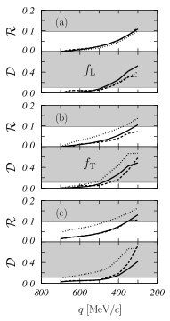
Figure 4: The ${\cal R}$ and ${\cal D}$ indexes calculated as in panel (d) of Fig. 2. In the panels (a) and (b) the $f_{\rm L}$ and $f_{\rm T}$ scaling functions calculated for the ¹²C nucleus are separately shown. In the panel (c) the indexes have been calculated by comparing the $f_{\rm L}$ and $f_{\rm T}$ scaling functions. The full lines represent the mean-field results, while the dotted and dashed lines have been obtained by doing continuum RPA calculations respectively with the polarization potential and with the Landau-Migdal interaction.

The scaling properties of continuum RPA $f_{\rm L}$ and $f_{\rm T}$ calculated for ¹²C are summarized in Fig. 4. The lines in this figure have been calculated with the same procedure used in the panel (d) of Fig. 2. The full lines represent the mean-field results, the dotted lines the results obtained with the finite-range interaction and the dashes lines have been obtained with the zero-range interaction. The figure shows that the scaling of first kind is well preserved by RPA calculations up to $q$=400 MeV/$c$. In the panel (c) the $f_{\rm L}$ and $f_{\rm T}$ scaling functions have been put together in the calculation of the two indexes. We observe a worsening of the scaling, especially for the polarization potential results. This indicates that the scaling of zeroth kind is slightly ruined by the RPA. This is understandable, since the effective nucleon-nucleon interaction acts in different manner on the longitudinal and on the transverse nuclear responses. Finally, the scaling of second kind is well preserved also in the RPA calculations.

III.3 Meson exchange currents

We have seen that collective excitations are different in longitudinal and transverse responses and this breaks the scaling of zeroth kind. However, our RPA results show that these effects are too small to explain the large differences between experimental $f_{L}$ and $f_{T}$ shown in Fig. 1. Another possible source of the breaking of the zeroth kind scaling are the MEC. Their role in the longitudinal responses is negligible Lallena (1996), while it can be relevant in the transverse responses.

Figure 5: Feynman diagrams of the MEC terms considered in our calculations. The (a) and (b) diagrams represent, respectively, the seagull and pionic currents, while the other two diagrams the $\Delta$ currents.

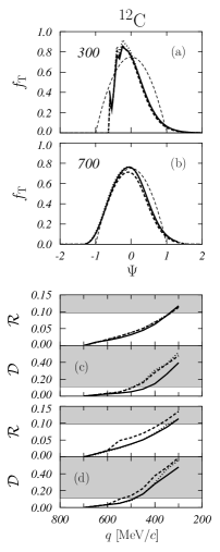
Figure 6: Transverse scaling functions for the ¹²C nucleus. In the (a) and (b) panels, the thin dashed lines show the RFG model. The other, thick, lines have been obtained by using the continuum shell model. The full lines show the results obtained by using one-body currents only. The dotted lines have been obtained by inserting the pionic and seagull terms of the MEC, and the dashed lines show the results obtained by including also the $\Delta$ currents. The numbers inside the panels indicate the values of the momentum transfer in MeV/$c$. The curves in the panels (c) and (d) are calculated as in panel (d) of Fig. 2. The curves in (c) compare the results obtained in ¹²C by using one-body currents only (full line) with those obtained by adding seagull and pionic MEC (dotted line) and by adding also the $\Delta$ currents (dashed lines). In panel (d) we compare the results obtained with all the MEC for the three nuclei considered. The full line show the ¹²C result, the dotted line the ¹⁶O result and the dashed line the ⁴⁰Ca result.

We have calculated the transverse response functions by adding to the one-body convection and magnetization currents the MEC arising from the exchange of a single pion. In Fig. 5 we show the Feynman diagrams of the MEC we have considered. They are the seagull, or contact, term, represented by the (a) diagram of the figure, where the virtual photon interacts at the pion-nucleon vertex, and the pionic, or pion in flight term, represented by the (b) diagram of the figure, where the virtual photon interacts with the exchanged pion. In addition we consider also the $\Delta$ current terms where the photon excites, or de-excites a virtual $\Delta$ resonance which interacts with another nucleon by exchanging a pion. These $\Delta$ current terms are represented by the (c) and (d) diagrams of Fig. 5. A detailed description of our MEC model is given in Refs. Anguiano et al. (2002, 2003, 2004).

We show in panels (a) and (b) of Fig. 6 the $f_{\rm T}$ scaling functions of the ¹²C nucleus calculated for the extreme $q$ values we have considered. The full lines have been obtained by using one-body currents only, the dotted lines by including seagull and pionic currents, and the dashed lines by adding the $\Delta$ currents. As usual, the thin dashed lines show the RFG scaling function.

The effects of the MEC on the scaling functions are analogous to those found on the responses in Ref. Amaro et al. (1994b). The seagull and pionic terms produce effects of opposite sign, therefore, the changes with respect to the one-body responses are rather small, and almost vanish for the largest values of $q$ we have considered. The inclusion of the $\Delta$ currents slightly decreases the values of the scaling functions. The presence of these currents becomes more relevant with increasing $q$ value.

The panel (c) of Fig. 6 shows the values of ${\cal R}$ and ${\cal D}$, calculated for $f_{\rm T}$ as in panel (d) of Fig. 2, for ¹²C. The meaning of the different curves is the same as in the two upper panels of the figure. In panel (d) we show the behaviour of the two indexes calculated for the $f_{\rm T}$ scaling functions when all the MEC are included. The full lines show the ¹²C results, the dotted lines the ¹⁶O results and the dashed lines the ⁴⁰Ca results.

Our MEC conserve rather well the scaling properties of $f_{\rm T}$. The shapes of the $f_{\rm T}$, shown in the upper panels of Fig. 6, are rather different from those of the empirical $f_{\rm T}$, given in Fig. 1. Our MEC model considers only virtual excitations of the $\Delta$ resonance which become more important at large $q$ values. All these observations indicate that the origin of the high energy tail of the experimental transverse scaling functions is the real excitation of the $\Delta$ resonance, with the consequent production of pions.

III.4 Short-range correlations and final state interactions

As already mentioned, we have also investigated the influence of SRC. Our results are summarized in Fig. 7, where, in the panel (a), we show, as example, the $f_{\rm L}$ scaling function of ¹²C calculated for $q$=700 MeV/$c$ with (dashed lines) and without (full curves) SRC. The same curves are plotted in both linear and logarithmic scales, to show the eventual effects in the tails of the distributions.

Figure 7: In the panel (a) we show the longitudinal scaling function of ¹²C calculated for $q$=700 MeV/$c$. The full lines show the mean-field result, the dashed lines have been obtained by including the SRC. In the insert, the same results are shown on a linear scale. In the panel (b) we show the momentum distribution of ¹²C calculated with the mean-field model, full line, and with the SRC, dashed line.

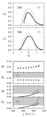
Figure 8: The same as Fig. 2 but showing the results of the mean field model with FSI.

The calculation of the responses with the SRC is done as described in Co’ and Lallena (2001), by considering all the cluster terms containing a single correlation line. This implies the evaluation of two and tree points cluster terms which produce contributions of different sign. The calculations have been done with the scalar correlation function labeled EU (Euler) in de Saavedra et al. (1996). The effects of the correlations on the momentum distribution of ¹²C are shown in the panel (b) of Fig. 7. Also this momentum distribution has been calculated in first order approximation de Saavedra et al. (1997). This example show that the scaling functions, in the kinematics of our interest, are insensitive to the high momentum tail of the momentum distribution, and, in general, to the SRC.

All the results we have so far presented, did not include the FSI which produce the largest modifications of the mean-field responses Amaro et al. (2001). We treat the FSI by using the model developed in Refs. Co’ et al. (1988); Smith and Wambach (1998). The mean-field responses are folded with Lorentz functions whose parameters have been extracted from optical potential volume integrals, and from the empirical spreading widths of single particle states. This approach has been successfully used to describe quasi-elastic electromagnetic responses Co’ et al. (1988); Amaro et al. (1994b), and, more recently, it has been applied to calculate neutrino scattering cross sections Bleve et al. (2001); Co’ et al. (2002); Botrugno and Co’ (2005).

In the two upper panels of Fig. 8 we show the shell model $f_{\rm L}$ scaling functions corrected for the presence of the FSI. Again, we show here the results obtained for the two extreme values of $q$ considered in our calculations. The thin dashed lines show the RFG results. It is evident that the FSI are responsible for the largest modifications of the mean-field results. The values of the maxima of the scaling functions in Fig. 2 are around 0.8. After the inclusion of the FSI, these maxima are of the order of 0.6. The FSI lower the values of the maxima of the responses, and, since the total area is conserved, increase their widths.

The presence of the FSI slightly worsen the almost perfect scaling of zeroth kind shown in Fig. 2. The FSI act differently on the two responses. The longitudinal responses are insensitive to the spin and spin-isospin terms of the nuclear interaction. This fact is considered in our FSI model. Even though in the panel (c) of Fig. 8 the values of ${\cal R}$, calculated for each $q$ value, are slightly larger than the analogous ones of Fig. 2, they are below the empirical value. The case of the ${\cal D}$ index is curious, since it shows almost constant values. This is because ${\cal D}$ indicates the maximum difference between the various curves considered. The FSI produce a smoothing of these curves and cancels the sharp resonant peaks which appear at low $q$ values.

The curves in the panel (d) are obtained in the same way as those of the analogous panel in Fig. 2. The values shown in Fig. 8 are clearly larger than those of panel (d) of Fig. 2. For the ${\cal R}$ index, the non scaling gray area is reached when the $q$ value is about 500 MeV/$c$. In conclusion, the FSI produce large modifications of the mean-field responses, but do not strongly violate the scaling.

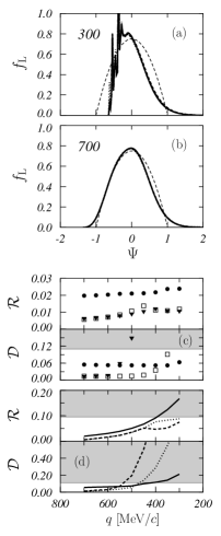
Figure 9: The same as Fig. 2 for the neutrino scaling functions. In both panels (a) and (b) the five scaling functions defined in Eqs. (20)-(24) and calculated for the ¹⁶O nucleus are shown by the thick lines. These lines are almost exactly overlapped. Again the dashed thin lines show the RFG scaling functions. In panel (c) the indexes are calculated by comparing the five scaling functions calculated at each $q$ value indicated on the $x$ axis. The black dots show the ¹²C results, the triangles the ¹⁶O results and the white squares the ⁴⁰Ca results. The values the two indexes shown in panel (d) have been calculated as in the analogous panel of Fig. 2. The full line refers to ¹²C, the dotted one to ¹⁶O and the dashed one to ⁴⁰Ca.

III.5 Neutrino scaling functions

Up to now, we have discussed the scaling properties of the electromagnetic scaling functions. We present in Fig. 9 the scaling functions defined in Eqs. (20)-(24), for the $(\nu_{e},e^{-})$ charge exchange reaction. The thick lines of the two upper panels show the five scaling functions calculated, in a continuum shell model, for the ¹⁶O nucleus, and for the two extreme values of $q$ considered in our work. The five curves are rather well overlapped at $q$=300 MeV/$c$, and almost exactly overlapped at $q$=700 MeV/$c$. The agreement with the RFG result, indicated as usual by the dashed thin lines, is rather good at $q$=700 MeV/$c$.

In panel (c) we show the ${\cal R}$ and ${\cal D}$ indexes calculated by comparing the five scaling functions at each $q$ value indicated in the $x$ axis. The black circles show the ¹²C results, the black triangles those of ¹⁶O and the white squares the ⁴⁰Ca results. These values are of the same order of magnitude as those of the (c) panel of Fig. 2. This confirms the observation that the scaling of zeroth kind is well satisfied in continuum shell model calculations.

In panel (d) the values of the two indexes are evaluated by doing a comparison of the scaling functions calculated at $q$=700 MeV/$c$ with those obtained for lower $q$ values. This indicates the validity of the scaling of first kind. The index ${\cal R}$ shows that there is a reasonable scaling down to $q$=400 MeV/$c$. This value is analogous to that found for the electromagnetic functions. The index ${\cal D}$ shows much rapid variations and, already at $q$=500 MeV/$c$, its value is over the empirical limiting value. This is due to the presence of sharp resonances at low $q$ values in some of the responses.

We studied the effects beyond the RFG for charge exchange neutrino responses, by following the same steps used for the electromagnetic responses. To be precise, we did not calculate responses with SRC or with the MEC, since from the results obtained for the electromagnetic responses, we do not expect large changes of the mean field results due to these effects. We found effects of RPA and FSI analogous to those of the electromagnetic case.

IV SUPERSCALING PREDICTIONS

In the previous section we have studied how the effects beyond the RFG model modify the scaling function. We found that the main effects are produced by the FSI. Despite the large modifications of the RFG scaling functions, the scaling properties are not heavily destroyed. For momentum transfer values above 500 MeV/$c$, our scaling functions present values of the scaling indexes smaller than the empirical benchmarks. After having established the range of validity of the superscaling hypothesis, we investigate, in this section, its prediction power. The strategy of our investigation consists in comparing responses, and cross sections, calculated by using RPA, FSI and eventually MEC and SRC, with those obtained by using our universal scaling functions, both $f_{\rm U}^{\rm ex}$ and $f_{\rm U}^{\rm th}$. All the RPA calculations presented in this section have been done by using the PP interaction.

Figure 10: Inclusive electron scattering cross sections. Here, the numbers in the panels indicate, in MeV, the energy of the incoming electron. The ¹²C data Sealock et al. (1989) have been measured at a scattering angle of $\theta$=37.5^o, the ¹⁶O data Anghinolfi et al. (1996) at $\theta$=32.0^o and the ⁴⁰Ca data Williamson et al. (1997) at $\theta$=45.5^o. The full lines show the results of our complete calculations. The cross sections obtained by using $f_{\rm U}^{\rm th}$ are shown by the dashed lines, and those obtained with $f_{\rm U}^{\rm ex}$ are given by the dotted lines.

Figure 11: Neutrino charge exchange cross sections on ¹⁶O. All the results shown in the various panels have been obtained for neutrino energy of 300 MeV. In all the panels the full lines show the result of our complete calculation, while the other lines show the results obtained by using the scaling functions. Specifically, the dashed and the dotted lines have been obtained respectively with $f_{\rm U}^{\rm th}$ and $f_{\rm U}^{\rm ex}$. In the panel (a) the double differential cross sections calculated for the scattering angle of 30^o as a function of the nuclear excitation energy is shown. In panel (b) we show the cross sections integrated on the scattering angle, always as a function of the nuclear excitation energy. In panel (c) we show the cross sections integrated on the nuclear excitation energy, as a function of the scattering angle.

Figure 12: Total neutrino cross sections. Both panels show the same results in linear (a) and logarithmic (b) scales. The full lines show the result of the complete calculations. The dashed lines have been obtained by using $f_{\rm U}^{\rm th}$, and the dotted lines by using $f_{\rm U}^{\rm ex}$.

The first test case of our study is done on the double differential electron scattering cross section. We show in Fig. 10 the inclusive electron scattering cross sections calculated with our model including the MEC and the FSI effects (full lines), those obtained with $f_{\rm U}^{\rm th}$ (dashed lines) and the cross sections obtained with $f_{\rm U}^{\rm ex}$ (dotted lines). These results are compared with the data of Refs. Sealock et al. (1989); Anghinolfi et al. (1996); Williamson et al. (1997).

The first remark about Fig. 10, regards the excellent agreement between the results of the full calculations with those obtained by using $f_{\rm U}^{\rm th}$. This clearly indicates the validity of the scaling approach in this kinematic region. This result was expected from the studies of the previous section, since in all the cases shown in Fig. 10, the value of the momentum transfer is larger than 500 MeV/$c$. The differences with the cross sections obtained by using the empirical scaling functions, reflect the differences between the various scaling functions shown in Fig. 1.

A second remark regarding Fig. 10, is about the fact that our results underestimate the data. Probably this is because the excitation of the $\Delta$ resonance is not considered in our calculations. The behaviour of the data of the figure in the higher energy part, show the presence of the $\Delta$ resonance. The low energy tail of the excitation of this resonance affect also the quasi-elastic peak.

The situation for the double differential cross sections is well controlled, since all the kinematic variables, beam energy, scattering angle, energy of the detected lepton, are precisely defined, and, consequently, also energy and momentum transferred to the nucleus. The situation changes for the total cross sections which are of major interest for the neutrino physics. The total cross sections are only function of the energy of the incoming lepton, therefore they consider all the scattering angles and the possible values of the energy and momentum transferred to the nucleus, with the only limitation of the global energy and momentum conservations. This means that, in the total cross sections, kinematic situations where the scaling is valid and also where it is not valid are both present.

In order to clarify this point with quantitative examples, we show in Fig. 11 various differential charge-exchange cross sections obtained for 300 MeV neutrinos on ¹⁶O target. In the panel (a) we show the double differential cross sections calculated for a scattering angle of 30^o, as a function of the nuclear excitation energy. The full line show the result of our complete calculation, done with continuum RPA and FSI. We have shown in the previous section that the effects of MEC and SRC are negligible, in this kinematic regime. The dashed line show the result obtained with $f_{\rm U}^{\rm th}$ and the dotted line with $f_{\rm U}^{\rm ex}$. The values of the momentum transfer vary from about 150 to 200 MeV/$c$. Evidently this is not the quasi-elastic regime where the scaling is supposed to hold, and this evidently produces the large differences between the various cross sections.

The cross sections integrated on the scattering angle are shown as a function of the nuclear excitation energy in the panel (b) of the figure, while the cross sections integrated on the excitation energy as a function of the scattering angle are shown in the panel (c).

The three panels of the figure illustrate in different manners the same physics issue. The calculation with the scaling functions fails in reproducing the results of the full calculation in the region of low energy and momentum transfer, where surface and collective effects are important. This is shown in panel (b) by the bad agreement between the three curves in the lower energy region, and in panel (c) at low values of the scattering angle, where the $q$ values are minimal.

Total charge-exchange neutrino cross sections are shown in Fig. 12 in both linear and logarithmic scale, as a function of the energy of the incident neutrino $\epsilon_{\rm i}$. As in the previous figure, the full lines show the result of the full calculation, while the dashed and dotted lines have been respectively obtained with $f_{\rm U}^{\rm th}$ and $f_{\rm U}^{\rm ex}$. The scaling predictions for neutrino energies up to 200 MeV are unreliable. These total cross sections are obviously dominated by the giant resonances, and more generally by collective nuclear excitation. We have seen that these effects strongly violate the scaling. At $\epsilon_{\rm i}$ =200 MeV the cross section obtained with $f_{\rm U}^{\rm th}$ is about 20% larger than those obtained with the full calculation. This difference becomes smaller with increasing energy and is about 7% at $\epsilon_{\rm i}$ = 300 MeV. This is an indication that the relative weight of the non scaling kinematic regions become smaller with the increasing neutrino energy.

V SUMMARY AND CONCLUSIONS

We have investigated the scaling properties of the electron and neutrino cross sections in a kinematic region involving momentum transfer values smaller than 700 MeV/$c$. Since our working methodology implies the numerical comparison of different scaling functions, we defined two indexes, Eqs. (32) and (33), to have a quantitative indication of the scaling quality.

We have first analyzed the scaling properties of the experimental electromagnetic responses given in Ref. Jourdan (1996) for the ¹²C, ⁴⁰Ca and ⁵⁶Fe nuclei. We found the better scaling situation for the longitudinal responses at 570 MeV/$c$. By considering these data we obtained empirical values of the two indexes which we consider the upper acceptable limit to have scaling. From a fit to the same set of data we have also obtained an empirical scaling function, $f_{\rm U}^{\rm ex}$.

Our study of the role played by effects beyond the RFG model on the scaling properties of the electroweak responses consisted in comparing the values of the indexes obtained in our calculations with the empirical values. We found that finite size effects conserve the scaling of first kind, the most likely violated, down to 400 MeV/$c$. We have estimated the effects of the collective excitations by doing continuum RPA calculations with two different residual interactions. The RPA effects become smaller the larger is the value of the momentum transfer. At momentum transfer values above 600 MeV/$c$ the RPA effects are negligible if calculated with a finite-range interaction, while zero-range interactions produce larger effects. Collective excitations breaks scaling properties. We found that scaling of first kind is satisfied down to about 500 MeV/$c$.

The presence of the MEC violates the scaling of the transverse responses. From the quantitative point of view, MEC effects, at relatively low $q$ values, are extremely small. In our model, MEC start to be relevant from $q\sim$ 600 MeV/$c$, especially these MEC related to the virtual excitation of the $\Delta$ resonance. In our calculations the real excitation of the $\Delta$ resonance, and the consequent production of real pions, is not considered. Our nuclear models deal with purely nucleonic degrees of freedom. Experimental transverse responses, such as those shown in Fig. 1, clearly show the presence of the $\Delta$ resonance peak, with increasing value of the momentum transfer. Our model indicates that MEC do not destroy the scaling in the kinematic range of our interest.

We have also investigated the effects of the SRC, which could also violate the scaling. However, the size of these effects are so small as to be negligible. The main modifications of the mean-field responses are due to the FSI. When we applied the FSI we obtain, even for $q$=700 MeV/$c$, scaling functions very different from those predicted by the RFG model or by the mean field model, and rather similar to the empirical one. In any case also the FSI do not heavily break the scaling properties. We found that the scaling of first kind is conserved down to $q$=450 MeV/$c$.

We have presented in detail only the results obtained for the electromagnetic transverse and longitudinal responses since we found for the weak responses, related to the neutrino scattering processes, analogous results. We can summarize the main points of this first part of our investigation by saying that the effects beyond the RFG model we have considered, strongly modify the scaling functions, but do not destroy their scaling. This explain the good scaling properties of the experimental longitudinal electromagnetic responses, which are not affected by the excitation of the $\Delta$ resonance, an effect not included in our calculations.

After studying the scaling properties of the various responses we have investigated the reliability of the cross sections predicted by using the scaling functions. The idea is to assume that superscaling is verified, i.e. all the three kinds of scaling we have considered, and then to use the scaling functions to predict the cross sections. The cross sections calculated with our complete model have been compared with those obtained by using as superscaling functions the empirical scaling function fitting the 570 MeV longitudinal data of Ref. Jourdan (1996) $f_{\rm U}^{\rm ex}$, and our longitudinal scaling function $f_{\rm U}^{\rm th}$. We have chosen this last scaling function as a theoretical universal scaling function.

We have verified that, in the quasi-elastic peak, the electron scattering cross sections obtained with the full calculation are very close to those obtained with $f_{\rm U}^{\rm th}$. Also the comparison with the data is rather good. These calculations have been done for momentum transfer values larger than 500 MeV/$c$, therefore these results confirm the validity of the superscaling in the quasi-elastic regime. The problems arise in the evaluation of the total neutrino cross sections. In these cross sections, together with the contribution of the quasi-elastic kinematics, where superscaling is satisfied, there is also the contribution of kinematics regions where there is not scaling. We found that the scaling predictions of the total neutrino cross sections are unreliable up to neutrino energies of 200 MeV. At this point the scaling cross sections are 20% larger than those obtained by the full calculation. This difference become smaller with increasing neutrino energy, and we found to be reduced to about the 7% at 300 MeV. We stopped here our calculations of the total cross section, since our model is not any reliable for larger neutrino energies. The comparison between double differential cross sections calculated at excitation energies of 150 and 200 MeV, for neutrino energies up to 1 GeV, gives an indication that the difference between the total cross sections becomes smaller with increasing neutrino energy. It is worth pointing out, however, that for neutrino energies larger than 300 MeV, the contribution of the $\Delta$ resonance is not any more negligible, as we have implicitly considered in our calculations.

Appendix A The experimental scaling functions

In this appendix we describe the procedure followed to obtain the experimental Scaling Functions (SF), and also the empirical values of the indexes ${\cal D}$ and ${\cal R}$, from the electromagnetic response data of Ref. Jourdan (1996).

The SF data have been obtained by inserting in Eqs. (7) and (8), the values of the experimental responses. The uncertainty on the SF data has been evaluated directly from the same equations, taking into account the uncertainties of the original response data.

The evaluation of ${\cal D}$ and ${\cal R}$, Eqs.(32) and (33), requires the knowledge of the various SF at the same $\Psi$ points. Since the SF data are given for different values of $\Psi$, we fixed a grid of $\Psi$ values, and we produced pseudo SF data by doing a quadratic interpolation of the SF data previously obtained.

The uncertainties of these pseudo SF data have been obtained by using a Monte Carlo strategy. Associated to each experimental SF point we have generated a new point compatible with the Gaussian distribution related to the experimental uncertainty. These new data formed a set of SF points used to obtain pseudo data on the grid by quadratic interpolation. We repeated this procedure thousand times, and obtained, for each value of $\Psi$ of the grid, a distribution of SF points which allowed us to determine the corresponding uncertainty.

After having determined the uncertainties of the pseudo SF data, we calculated the uncertainty of the ${\cal D}$ index as:

$$\sigma_{{\cal D}}\,=\,\sqrt{[f^{\rm max}_{i}(\psi_{i_{\rm max}})]^{2}+[f^{\rm min}_{i}(\psi_{i_{\rm max}})]^{2}}\,,$$

where $\Psi_{i_{\rm max}}$ is the value where the difference $f^{\rm max}_{i}-f^{\rm min}_{i}$ reaches the maximum value.

We have calculated the uncertainty on ${\cal R}$ in two steps. We first evaluated the uncertainty of the sum

$$S\,=\,\sum_{i=1,\ldots,K}\left[f^{\rm max}_{i}-f^{\rm min}_{i}\right]\,,$$

in the numerator of Eq. (33) by using a procedure analogous to that used to obtain $\sigma_{\cal D}$. That is,

$$\sigma_{S}\,=\,\sqrt{\sum_{i=1,\ldots,K}\left([f^{\rm max}_{i}]^{2}+[f^{\rm min}_{i}]^{2}\right)}\,.$$

To obtain the global uncertainty, we used again a Monte Carlo strategy, and we calculated the ratio in Eq. (33) thousand times by sampling the values of $S$ and of $f^{\rm max}$ within the corresponding Gaussian distributions.

The empirical SF represented by the thin full line in the $f_{\rm L}$ panel at 570 MeV/$c$ in Fig. 1, has been obtained as a best fit of all the experimental points shown in the panel. The expression of our fitting function is:

$$f_{\rm U}^{\rm ex}(\Psi)\,=\,\frac{A\exp(-\Psi^{2})+B\Psi^{2}+C\Psi+D}{(\Psi+E)^{2}+F^{2}}\,.$$ (37)

with $A$= 0.971, $B$=-0.067, $C$= 0.385, $D$= 0.145, $E$= 0.366, $F$= 1.378.

References

- Alberico et al. (1988) W. M. Alberico, A. Molinari, T. W. Donnelly, E. L. Kronenberg, and J. W. Van Orden, Phys. Rev. C 38, 1801 (1988).
- DePace (1998) A. De Pace, Nucl. Phys. A 635, 163 (1998).
- Amaro et al. (2002) J. E. Amaro, M. B. Barbaro, J. A. Caballero, T. W. Donnelly, and A. Molinari, Phys. Rep. 368, 317 (2002).
- Maieron et al. (2002) C. Maieron, T. W. Donnelly, and I. Sick, Phys. Rev. C 65, 025502 (2002).
- Amaro et al. (2005a) J. E. Amaro, M. B. Barbaro, J. A. Caballero, T. W. Donnelly, A. Molinari, and I. Sick, Phys. Rev. C 71, 015501 (2005a).
- Amaro et al. (2005b) J. E. Amaro, M. B. Barbaro, J. A. Caballero, T. W. Donnelly, and C. Maieron, Phys. Rev. C 71, 065501 (2005b).
- Donnelly and Sick (1999a) T. W. Donnelly and I. Sick, Phys. Rev. Lett. 82, 3212 (1999a).
- Donnelly and Sick (1999b) T. W. Donnelly and I. Sick, Phys. Rev. C 60, 065502 (1999b).
- Jourdan (1996) J. Jourdan, Nucl. Phys. A 603, 117 (1996).
- Barbaro et al. (1998) M. B. Barbaro, R. Cenni, A. De Pace, T. W. Donnelly, and A. Molinari, Nucl. Phys. A 643, 137 (1998).
- Barbaro et al. (2004) M. B. Barbaro, J. A. Caballero, T. W. Donnelly, and C. Maieron, Phys. Rev. C 69, 035502 (2004).
- Amaro et al. (2006) J. E. Amaro, M. B. Barbaro, J. A. Caballero, and T. W. Donnelly, Phys. Rev. C 73, 035503 (2006).
- Antonov et al. (2006) A. N. Antonov, M. V. Ivanov, M. K. Gaidarov, E. Moya de Guerra, P. Sarriguren, and J. M. Udías, Phys. Rev. C 73, 047302 (2006).
- Boffi et al. (1996) S. Boffi, C. Giusti, F. Pacati, and M. Radici, Electromagnetic response of atomic nuclei (Clarendon, Oxford, 1996).
- Edmonds (1957) A. R. Edmonds, Angular momentum in quantum mechanics (Princeton University Press, Princeton, 1957).
- Blatt and Weisskopf (1952) J. M. Blatt and V. F. Weisskopf, Theoretical nuclear physics (John Wiley and sons, New York, 1952).
- Hoeler et al. (1976) G. Hoeler, E. Pietarinen, I. Sabba-Stefanescu, F. Borkowski, G. G. Simon, V. H. Walther, and R. D. Wendling, Nucl. Phys. B 114, 505 (1976).
- Amaro et al. (1996) J. E. Amaro, J. A. Caballero, T. W. Donnelly, A. M. Lallena, E. Moya de Guerra, and J. Udías, Nucl. Phys. A 602, 263 (1996).
- O’Connell et al. (1972) J. S. O’Connell, T. W. Donnelly, and J. D. Walecka, Phys. Rev. C 6, 719 (1972).
- Walecka (1975, p. 113) J. D. Walecka, in Muon Physics, vol.2, V.W. Huges, C.S. Wu (Eds) (Academic Press, New York, 1975, p. 113).
- Walecka (1995) J. D. Walecka, Theoretical nuclear and subnuclear physics (Oxford University Press, New York Oxford, 1995).
- Amaro et al. (1994a) J. E. Amaro, G. Co’, and A. M. Lallena, Int. J. Mod. Phys. E 3, 735 (1994a).
- Botrugno and Co’ (2005) A. Botrugno and G. Co’, Nucl. Phys. A 761, 203 (2005).
- de Saavedra et al. (1996) F. Arias de Saavedra, G. Co’, A. Fabrocini, and S. Fantoni, Nucl. Phys. A 605, 359 (1996).
- Pines et al. (1998) D. Pines, K. Q. Quader, and J. Wambach, Nucl. Phys. A 477, 365 (1998).
- Fetter and Walecka (1971) A. L. Fetter and J. D. Walecka, Quantum theory of many-particle systems (McGraw-Hill, S. Francisco, 1971).
- Lallena (1996) A. M. Lallena, Nucl. Phys. A 615, 325 (1996).
- Anguiano et al. (2002) M. Anguiano, G. Co’, A. M. Lallena, and S. R. Mokhtar, Ann. Phys. (N.Y.) 296, 235 (2002).
- Anguiano et al. (2003) M. Anguiano, G. Co’, and A. M. Lallena, J. Phys. G 29, 1119 (2003).
- Anguiano et al. (2004) M. Anguiano, G. Co’, and A. M. Lallena, Nucl. Phys. A 744, 2004 (2004).
- Amaro et al. (1994b) J. E. Amaro, G. Co’, and A. M. Lallena, Nucl. Phys. A 578, 365 (1994b).
- Co’ and Lallena (2001) G. Co’ and A. M. Lallena, Ann. Phys. (N.Y.) 287, 101 (2001).
- de Saavedra et al. (1997) F. Arias de Saavedra, G. Co’, and M. M. Renis, Phys. Rev. C 55, 673 (1997).
- Amaro et al. (2001) J. E. Amaro, G. Co’, and A. M. Lallena, Quasielastic electron scattering in nuclei, R. Cenni Ed. (Nova Science, New York, 2001).
- Co’ et al. (1988) G. Co’, K. F. Quader, R. D. Smith, and J. Wambach, Nucl. Phys. A 485, 61 (1988).
- Smith and Wambach (1998) R. D. Smith and J. Wambach, Phys. Rev. C 38, 100 (1998).
- Bleve et al. (2001) C. Bleve, G. Co’, I. De Mitri, P. Bernardini, G. Mancarella, D. Martello, and A. Surdo, Astrop. Phys. 16, 145 (2001).
- Co’ et al. (2002) G. Co’, C. Bleve, I. De Mitri, and D. Martello, Nucl. Phys. B (Proc. Suppl.) 112, 210 (2002).
- Sealock et al. (1989) R. M. Sealock et al., Phys. Rev. Lett. 62, 1350 (1989).
- Anghinolfi et al. (1996) M. Anghinolfi et al., Nucl. Phys. A 602, 405 (1996).
- Williamson et al. (1997) C. Williamson et al., Phys. Rev. C 56, 3152 (1997).