Nuclear polarizability of helium isotopes in atomic transitions

Abstract

We estimate the nuclear polarizability correction to atomic transition frequencies in various helium isotopes. This effect is non-negligible for high precision tests of quantum electrodynamics or accurate determination of the nuclear charge radius from spectroscopic measurements in helium atoms and ions, in particular it amounts to $28(3)$ kHz for 1S-2S transition in ⁴He⁺.

There are various corrections which need to be included in an accurate calculation of the atomic energy levels. These are relativistic and QED effects, finite nuclear mass and, to some extent, finite nuclear size. There is also an additional correction which comes from possible nuclear excitation due to the electric field of the surrounding electrons. This effect is usually neglected, as it is relatively small compared to the uncertainties in the nuclear charge radii. There are however exceptions, where the nuclear polarizability correction can be significant. The first known example was the $2P_{3/2}-2S_{1/2}$ transition in muonic helium $\mu$-⁴He⁺ bj ; friar_m , where the polarizability correction is about 1% of the finite nuclear size effect. Another example is the isotope shift in the $1S-2S$ transition frequency between hydrogen and deuterium. The nuclear polarizability correction of about $20$ kHz, was two orders of magnitude larger than the experimental precision huber , and helped to resolve experimental discrepancies for the deuteron charge radius. Another very recent example is the isotope shift in the $2S-3S$ transition frequency between ¹¹Li and ⁷Li 11li . The ¹¹Li nucleus has probably the largest nuclear polarizability among all light nuclei, with a contribution to the $2S-3S$ isotope shift of about $36$ kHz. In this paper we study in detail the nuclear polarizability correction to atomic transitions for helium isotopes: ³He, ⁴He and ⁶He and compare with currently available and planned accurate measurements of transition frequencies in helium atoms and ions.

The interaction of the nucleus with an electromagnetic field can be described by the following Hamiltonian:

$$H_{\rm int}=q\,A^{0}-\vec{d}\cdot\vec{E}-\vec{\mu}\cdot\vec{B}-\frac{q}{6}\,\langle r^{2}\rangle\,\nabla\cdot\vec{E},$$ (1)

which is valid as long as the characteristic momentum of the electromagnetic field is smaller than the inverse of the nuclear size. Otherwise, one has to use a complete description in terms of formfactors and structure functions. Under this assumption, the dominant term for the nuclear excitation is the electric dipole interaction. This is the main approximation of our approach, which may not always be valid. It was checked however that higher order polarizabilities are quite small (below 1 kHz) for deuterium ros ; friar , and this should be similar for He isotopes. Within this low electromagnetic momentum approximation, the nuclear polarizability correction to the energy is given by the following formula mp (in units $\hbar=c=1,e^{2}=4\,\pi\,\alpha$):

$$E_{\rm pol}=-m\,\alpha^{4}\,\Bigl{\langle}\sum_{a}\delta^{3}(r_{a})\Bigr{\rangle}\;(m^{3}\,\tilde{\alpha}_{\rm pol}),$$ (2)

where $m$ is the electron mass and the expectation value of the Dirac $\delta$ is taken with the electron wave function in atomic units. For hydrogenic systems it is equal to $Z^{3}/\pi$. In the equation above, $\tilde{\alpha}_{\rm pol}$ is a weighted electric polarizability of the nucleus, which is given by the following double integral

$$\tilde{\alpha}_{\rm pol} = \frac{16\,\alpha}{3}\,\int_{E_{T}}^{\infty}dE\,\frac{1}{e^{2}}\,|\langle\phi_{N}|\vec{d}|E\rangle|^{2}\,\int_{0}^{\infty}\,\frac{dw}{w}\,\frac{E}{E^{2}+w^{2}}$$ (3)

$$\times\frac{1}{(\kappa+\kappa^{\star})}\,\biggl{[}1+\frac{1}{(\kappa+1)(\kappa^{\star}+1)}\,\biggl{(}\frac{1}{\kappa+1}+\frac{1}{\kappa^{\star}+1}\biggr{)}\biggr{]}$$

where $\kappa=\sqrt{1+2\,i\,m/w}$ and $E_{T}$ is the excitation energy for the breakup threshold. The kets $|\phi_{N}\rangle$ and $|E\rangle$ denote the ground state of the nucleus and a dipole excited state with excitation energy $E$, respectively. The square of the dipole moment is related to the so called $B(E1)$ function by

$$|\langle\phi_{N}|\vec{d}|E\rangle|^{2}=\frac{4\,\pi}{3}\,\frac{dB(E1)}{dE}$$ (4)

in units $e^{2}$ fm² MeV^-1, which explains the presence of $e^{2}$ in the denominator in Eq. (3). The $B(E1)$ function is, in turn, directly related to the photoabsorption cross section at photon energies $E$

$$\sigma(E)=\frac{16\,\pi^{3}}{9}\,\alpha\,E\,\left(\frac{1}{e^{2}}\,\frac{dB(E1)}{dE}\right)$$ (5)

which allows us to obtain the $B(E1)$ function from experimental data.

If $E_{T}$ is much larger than the electron mass $m$, one can perform a small electron mass expansion and obtain a simplified formula, in agreement with that previously derived in weitz :

$$\tilde{\alpha}_{\rm pol} = \frac{19}{6}\,\alpha_{\rm E}+5\,\alpha_{\rm Elog}$$ (6)

$$\alpha_{\rm E} = \frac{2\,\alpha}{3}\,\frac{1}{e^{2}}\,\biggl{\langle}\phi_{N}\biggl{|}\,\vec{d}\,\frac{1}{H_{N}-E_{N}}\,\vec{d}\;\biggr{|}\phi_{N}\biggr{\rangle}$$ (7)

$$= \frac{8\,\pi\,\alpha}{9}\,\int_{E_{T}}\frac{dE}{E}\,\frac{1}{e^{2}}\frac{dB(E1)}{dE}$$

$$\alpha_{\rm Elog} = \frac{2\,\alpha}{3}\,\frac{1}{e^{2}}\,\biggl{\langle}\phi_{N}\biggl{|}\,\vec{d}\,\frac{1}{H_{N}-E_{N}}\,\ln\biggl{(}\frac{2(H_{N}-E_{N})}{m}\biggr{)}\,\vec{d}\;\biggr{|}\phi_{N}\biggr{\rangle}$$ (8)

$$= \frac{8\,\pi\,\alpha}{9}\,\int_{E_{T}}\frac{dE}{E}\,\frac{1}{e^{2}}\frac{dB(E1)}{dE}\,\ln\biggl{(}\frac{2\,E}{m}\biggr{)}\,,$$

where $\alpha_{\rm E}$ is the static electric dipole polarizability and $\alpha_{\rm Elog}$ is the logarithmically modified polarizability. We have tested this approximation for ³He and ⁴He isotopes, and found that numerical results differ from the exact formula in Eq. (3) by less than $0.1\%$.

In the opposite situation, i.e.  when $m$ is much larger that $E_{T}$, that corresponds to the nonrelativistic limit, the polarizability correction adopts the form (with $m$ being the reduced mass here):

$$E_{\rm pol}=-m\,\alpha^{4}\,\Bigl{\langle}\sum_{a}\delta^{3}(r_{a})\Bigr{\rangle}\;\frac{32\,\pi\,\alpha\,m^{2}}{9}\,\int_{E_{T}}dE\,\frac{1}{e^{2}}\frac{dB(E1)}{dE}\,\sqrt{\frac{m}{2\,E}}.$$ (9)

This approximation is justified for muonic helium atoms or ions, because the muon mass ($\sim 106$ MeV) is much larger than the threshold energy $E_{T}$ [see Eq. (10)]. This formula requires, however few significant corrections, namely Coulomb distortion and formfactor corrections. They were obtained by Friar in friar_m for the calculation of the polarizability correction in $\mu\,^{4}$He. This nonrelativistic approximation, however, is not valid for electronic atoms since the typical nuclear excitation energy in light nuclei is larger than the electron mass.

We consider in this work three helium isotopes, namely ³He, ⁴He and ⁶He, which are stable or sufficiently long lived for performing precise atomic measurements. The separation energy $S\equiv E_{T}$ for these helium isotopes are audi :

$$S_{2n}(^{6}{\rm He}) = 0.975\,{\rm MeV}\,,$$

$$S_{p}(^{4}{\rm He}) = 19.8\,{\rm MeV}\,,$$

$$S_{n}(^{4}{\rm He}) = 20.6\,{\rm MeV}\,,$$ (10)

$$S_{p}(^{3}{\rm He}) = 5.493\,49\,{\rm MeV}\,,$$

$$S_{n}(^{3}{\rm He}) = 7.718\,04\,{\rm MeV}\,.$$

The separation energy $S$ is the main factor which determines the magnitude of the nuclear polarizability correction, since $E_{\rm pol}$ is approximately proportional to the inverse of $S$.

We first consider the ⁶He isotope. In this case the polarizability $\tilde{\alpha}(^{6}{\rm He})$ was calculated from two different $B(E1)$ distributions. The first one corresponds to the experimental distribution extracted by Aumann et al. Aum99 from the Coulomb breakup of ⁶He on lead at 240 MeV/u. These data are represented by the dots in Fig. 1. The second $B(E1)$ distribution corresponds to a theoretical calculation, and was obtained in Tho00 by evaluating the matrix element of the dipole operator between the ground state and the $1^{-}$ continuum states. These states where obtained by solution of the Schrödinger equation, assuming a three-body model for the ⁶He nucleus, with pairwise neutron-neutron and neutron-$\alpha$ interactions, plus an effective three-body force. The $B(E1)$ obtained in this calculation is represented in Fig. 1 by the dashed line.

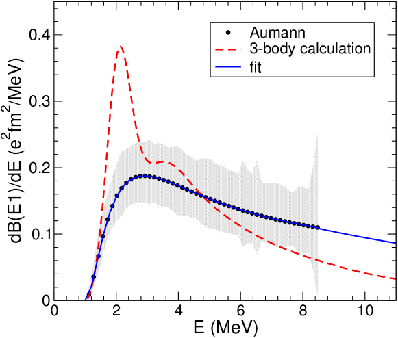
Figure 1: Electric dipole line strength $dB(E1)/dE$ in units $e^{2}\,{\rm fm}^{2}/$MeV for ⁶He. The solid line is a fit to the experimental distribution of Aumann et al. Aum99 (filled circles), extrapolated to 12 MeV. The shadow region indicates the experimental uncertainty of the data. The dashed line is the calculation of Thompson et al. Tho00 .

In spite of the discrepancy between the theoretical and the experimental $B(E1)$ distributions, the deduced polarizability $\tilde{\alpha}_{\rm pol}$, as obtained from Eq. (3), is similar in both cases: $\tilde{\alpha}_{\rm pol,the}=24.2\,{\rm fm}^{3}$ versus $\tilde{\alpha}_{\rm pol,exp}=21.1\,{\rm fm}^{3}$. It should be noted that the experimental data were extrapolated and integrated up to $E_{T}=12.3$ MeV, the threshold value for the decay into two tritons. We do not have, however, experimental data for the $B(E1)$ beyond this threshold. Therefore, for the final result we take the average and add the polarizability of ⁴He [calculated in Eq. (16)] to partially account for other decay channels, and obtain

$$\tilde{\alpha}_{\rm pol}(^{6}{\rm He})=24.7(5.0)\,{\rm fm}^{3}=4.3(9)\cdot 10^{-7}\;m^{-3}\,,$$ (11)

where $m$ is the electron mass. For the comparison with other possible determinations of ⁶He polarizabilities, we additionally present in Table I the static electric dipole and logarithmically modified polarizabilities. However, they can not be used to determine $\tilde{\alpha}_{\rm pol}$ since the $E_{T}$ is of the order of the electron mass $m$.

	Ref.	$\alpha_{\rm E}$[fm3]	$\alpha_{\rm Elog}$[fm3]	$\tilde{\alpha}_{\rm pol}$[fm3]
3He		$0.153(15)$	$0.615(62)$	$3.56(36)$
	rinker	$0.130(13)$
	leid	$0.145$
	goec	$0.250(40)$
4He		$0.076(8)$	$0.365(37)$	$2.07(20)$
	leid	$0.076$
	gazit	$0.0655$
	friar_m	$0.072(4)$
6He		$1.99(40)$	$4.78(96)$	$24.7(5.0)$

Table 1: The electric dipole polarizability $\alpha_{\rm E}$, the logarithmically modified polarizability $\alpha_{\rm Elog}$, and the weighted polarizability $\tilde{\alpha}_{\rm pol}$ for helium isotopes.

The resulting contribution to the frequency of, for example, the $2^{3}S_{1}-3^{3}P_{2}$ transition in ⁶He is

$$E_{\rm pol} = -m\,\alpha^{4}\,\Bigl{\langle}\delta^{3}(r_{1})+\delta^{3}(r_{2})\Bigr{\rangle}_{2^{3}S_{1}-3^{3}P_{2}}\;(m^{3}\,\tilde{\alpha}_{\rm pol})=h\,\nu_{\rm pol}\,\,.$$ (12)

$$\nu_{\rm pol} = 0.015(3)\,{\rm MHz}\,.$$ (13)

For comparison, the finite nuclear size correction to the same transition is Wan04 :

$$E_{\rm fs} = \frac{2\,\pi}{3}\,Z\,\alpha^{4}\,m^{3}\,\langle r_{\rm ch}^{2}\rangle\,\Bigl{\langle}\delta^{3}(r_{1})+\delta^{3}(r_{2})\Bigr{\rangle}_{2^{3}S_{1}-3^{3}P_{2}}=h\,\nu_{\rm fs}\,\,.$$ (14)

$$\nu_{\rm fs} = -1.008\,\langle r_{\rm ch}^{2}\rangle\frac{\rm MHz}{{\rm fm}^{2}}=-4.253\,{\rm MHz}\,\,.$$ (15)

The relative magnitude of the nuclear polarizability to the nuclear finite size for ⁶He is about $0.35$ %, so it alters the charge radius determination at this precision level. However, the uncertainty of the experimental result of Wang et al. Wan04 for the isotope shift between ⁶He and ⁴He, $\nu_{\rm iso}=43\,194\,772(56)$ kHz, is about four times larger than $\nu_{\rm pol}$, and therefore the nuclear polarizability correction at this precision level is not very significant.

We proceed now to evaluate the ⁴He nuclear polarizability. This has been obtained from the total photoabsorption cross section measured by Arkatov et al. Ark78 ; Ark80 ; Fuh95 .

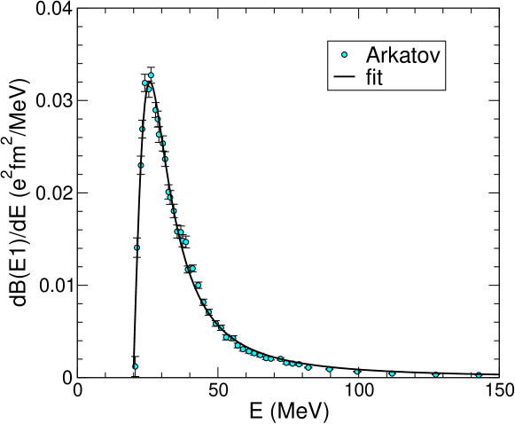
Figure 2: Electric dipole line strength $dB(E1)/dE$ in units $e^{2}\,{\rm fm}^{2}/$MeV for ⁴He. The circles correspond to the data of Arkatov et al. Ark78 ; Ark80 ; Fuh95 . The solid line is a fit to the data.

Using Eq. (5), we extracted from these data the $B(E1)$ distribution shown in Fig. 2 (filled circles). Then, applying Eq. (6), one obtains the weighted polarizability of ⁴He:

$$\tilde{\alpha}({{}^{4}}{\rm He})=2.07(20)\,{\rm fm}^{3}=3.6(4)\,10^{-8}\,m^{-3}\,.$$ (16)

It should be noted that at $100$ MeV the dipole approximation in Eq. (1) may not be correct, since the corresponding photon wavelength is of order of the nuclear size. Therefore we introduce $10\%$ uncertainty to account for this approximate treatment. Results for the static polarizability obtained in this work, along with those obtained in other works, are presented in Table I. Our static polarizability agrees with that of Friar friar_m , which was based on earlier experimental data for the photoproduction cross section. It agrees also with theoretical calculations by Leidemann leid , but slightly disagrees with the most recent calculations of Gazit et al gazit .

The obtained weighted polarizability gives a relatively small effect for transitions in neutral helium. The ratio of the polarizability to the finite size correction is $4.6\cdot 10^{-4}$. At present, there are no measurements for the charge radii at this precision level. However, from the planned high precision measurement of the $1S-2S$ transition in ⁴He⁺ hansch , one can in principle obtain the charge radius of the $\alpha$ particle from the knowledge of the nuclear polarizability. The polarizability correction to this transition amounts to

$$\nu_{\rm pol}(1S-2S,{\rm{}^{4}He}^{+})=28(3)\,{\rm kHz}$$ (17)

and is smaller than the uncertainty of about $400$ kHz in current theoretical predictions, which are due to $\alpha^{2}\,(Z\,\alpha)^{6}$ higher order two-loop electron self-energy corrections yerokhin .

For the ³He atom, we separately calculate the nuclear polarizability corrections coming from the two- and three-body photodisintegration processes. There are many experimental results for the photoabsorption cross section as well as theoretical calculations. They agree fairly well for the two-body dissociation, but they significantly differ for the case of three-body disintegration at high excitation energies ($E_{\gamma}>20$ MeV). Since these experimental results have large uncertainties we prefer to rely on theoretical calculations which agree with each other very well. In this work, we will use the calculations of Deltuva et al. Del05 and Golak et al. Gol05 . The former uses the realistic CD Bonn NN potential, supplemented with a three-body force to account for the $\Delta$ excitation, and a full treatment of the Coulomb potential. The calculation of Golak et al. is based on the AV18 NN interaction in combination with the UrbanaIX three-nucleon force, and considers Coulomb effects just for the ground state. The $B(E1)$ distributions, extracted from these theoretical photodisintegration cross sections, are displayed in Figs. 3 and 4, respectively, as a function of the excitation energy.

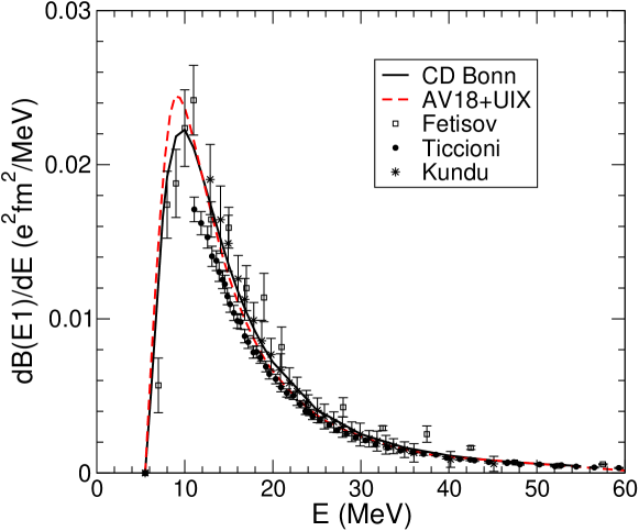
Figure 3: Electric dipole line strength $dB(E1)/dE$ in units $e^{2}\,{\rm fm}^{2}/$MeV for two-body disintegration of ³He. The data are from Fetisov et al. Fet65 , Ticcioni et al. Tic73 and Kundu et al. Kun71 . The solid and dashed lines are the calculations by Deltuva et al. Del05 and Golak et al. Gol05 , respectively.

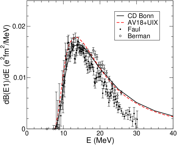
Figure 4: Electric dipole line strength $dB(E1)/dE$ in units $e^{2}\,{\rm fm}^{2}/$MeV for three-body disintegration of ³He. The data are from Faul et al. Fau81 and Berman et al. Ber74 . The solid and dashed lines are the calculations by Deltuva et al. Del05 and Golak et al. Gol05 , respectively.

Using these theoretical $B(E1)$ distributions, the result for the weighted polarizability due to both two- and three-body disintegration is

$$\tilde{\alpha}({\rm{}^{3}He})=3.56(36)\,{\rm fm}^{3}=6.2(6)\,10^{-8}\,m^{-3},$$ (18)

and the related contribution to the frequency of the $1S-2S$ transition in He⁺ is

$$\nu_{\rm pol}(1S-2S,{\rm{}^{3}He}^{+})=48(5)\,{\rm kHz}.$$ (19)

Hence, the magnitude of the nuclear polarizability correction for ³He is almost twice as large as for ⁴He and can be significant for the absolute charge radius determination from the $1S-2S$ measurement in hydrogen-like helium. The corresponding contribution to the ⁴He-³He isotope shift in the $2^{3}S_{1}-2^{3}P_{J}$ transition of $-1$ kHz is at present much smaller than the experimental precision of about $30$ kHz 3he .

Our result for the static polarizability of ³He is presented in Table I. It is in agreement with the first calculation by Rinker rinker which was based on measured that time photoabsorption cross section, it is also in agreement with calculations of Leidemann leid , but is in disagreement with the cross section mesurement for the elastic scattering of ³He nuclei of ²⁰⁸Pb below the Coulomb barrier goec .

In summary, we have obtained the nuclear polarizability correction in helium isotopes. In most cases, we find that the correction to the energy levels is smaller than current experimental precision, but could affect the determination of the charge radius when more accurate measurements become available. Together with possible high precision measurements in muonic atoms, it will allow for an improved test of QED and a more accurate determination of the fundamental constants.

References

- (1) J. Bernabéu and C. Jarlskog, Nucl. Phys. B47, 205 (1974).
- (2) J.L. Friar, Phys. Rev. C 16, 1540 (1977).
- (3) A. Huber, et al., Phys. Rev. Lett. 80, 468 (1998).
- (4) R. Sánchez, et al., Phys. Rev. Lett. 96, 033002 (2006).
- (5) W. Leidemann and R. Rosenfelder, Phys. Rev. C 51, 427 (1995).
- (6) J.L. Friar and G.L. Payne, Phys. Rev. C 56, 619 (1997).
- (7) M. Puchalski, A. Moro and K. Pachucki, Phys. Rev. Lett. 97, 133001 (2006).
- (8) K. Pachucki, D. Leibfried, and T.W. Hänsch, Phys. Rev. A 48, R1 (1993); K. Pachucki, M. Weitz, and T.W. Hänsch, Phys. Rev. A 49, 2255 (1994).
- (9) G. Audi, A.H. Wapstra, and C. Thibault, Nucl. Phys. A729, 337 (2003).
- (10) T. Aumann et al., Phys. Rev. C 59, 1252 (1999).
- (11) I.J. Thompson, B.V. Danilin, V.D. Efros, J.S. Vaagen, J.M. Bang and M.V. Zhukov, Phys. Rev. C 61, 024318 (2000).
- (12) G.A. Rinker, Phys. Rev. A 14, 18 (1976).
- (13) W. Leidemann, Few-Body Syst. Suppl. 14, 313 (2003).
- (14) F. Goeckner, L.O. Lamm, and L.D. Knutson, Phys. Rev. C 43, 66 (1991).
- (15) D. Gazit, N. Barnea, S. Bacca, W. Leidemann, and G. Orlandini, Phys. Rev. C 74, 061001(R) (2006); D. Gazit, S. Bacca, N. Barnea, W. Leidemann, and G. Orlandini, Phys. Rev. Lett. 96, 112301 (2006).
- (16) L.-B. Wang et al., Phys. Rev. Lett. 93, 142501 (2004).
- (17) J.M. Arkatov, P.I. Vatset, V.I. Voloshchuk, V.N. Gurev, A.F. Khodyachikh, Ukr. Fiz. Zh. 23, 1818 (1978).
- (18) Yu.M. Arkatov, P.I. Vatset, V.I. Voloshchuk, V.A. Zolenko, I.M. Prokhorets, Yad. Fiz. 31, 1400 (1980); [Sov. J. Nucl. Phys. 31, 726 (1980)].
- (19) K. Fuhrberg et al., Nucl. Phys. A 591, 1 (1995).
- (20) G. Gohle et al., Nature 436, 234 (2005).
- (21) V.A. Yerokhin, P. Indelicato, and V.M. Shabaev, Phys. Rev. A 71, 040101(R) (2005).
- (22) A. Deltuva, A.C. Fonseca, and P.U. Sauer, Phys. Rev. C 71, 054005 (2005); ibid 72, 054004 (2005).
- (23) J. Golak, R. Skibiński, H. Witała, W. Glöckle, A. Nogga, H. Kamada, Phys. Rep. 415, 89 (2005).
- (24) V.N. Fetisov, A.N. Gorbunov, and A.T.Varfolomeev, Nucl. Phys. 71, 305 (1965).
- (25) G. Ticcioni, S.N. Gardiner, J.L. Matthews, and R.O. Owens, Phys. Lett. 46B, 369 (1973).
- (26) S.K. Kundu, Y.M. Shin, G.D. Wait, Nucl. Phys. A 171, 384 (1971).
- (27) D.D. Faul, B.L. Berman, P. Meyer, and D.L. Olson, Phys. Rev. C 24, 849 (1981).
- (28) B.L. Berman, S.C. Fultz, P.F. Yergin, Phys. Rev. C 10, 2221 (1974).
- (29) D.C. Morton, Q. Wu, and G.W.F. Drake, Phys. Rev. A 73, 034502 (2006).