Extended Theory of Finite Fermi Systems:
Application to the collective and non-collective E1 strength in ²⁰⁸Pb

Abstract

The Extended Theory of Finite Fermi Systems is based on the conventional Landau-Migdal theory and includes the coupling to the low-lying phonons in a consistent way. The phonons give rise to a fragmentation of the single-particle strength and to a compression of the single-particle spectrum. Both effects are crucial for a quantitative understanding of nuclear structure properties. We demonstrate the effects on the electric dipole states in ²⁰⁸Pb (which possesses $50\%$ more neutrons then protons) where we calculated the low-lying non-collective spectrum as well as the high-lying collective resonances. Below 8 MeV, where one expects the so called isovector pygmy resonances, we also find a strong admixture of isoscalar strength that comes from the coupling to the high-lying isoscalar electric dipole resonance, which we obtain at about 22 MeV. The transition density of this resonance is very similar to the breathing mode, which we also calculated. We shall show that the extended theory is the correct approach for self-consistent calculations, where one starts with effective Lagrangians and effective Hamiltonians, respectively, if one wishes to describe simultaneously collective and non-collective properties of the nuclear spectrum. In all cases for which experimental data exist the agreement with the present theory results is good.

PACS: 24.30.Cz; 21.60.Ev; 27.40.+z

Keywords: Microscopic theory, low-lying and high-lying isoscalar and isovector electric dipole strength, Single-particle continuum, Transition densities.

I Introduction

The structure of neutron-rich nuclei is important for many applications in astrophysics. The rapid neutron-capture process, for instance, requires detailed knowledge of the properties of nuclei between the valley of stability and the neutron drip-line, such as neutron capture rates or photon-induced neutron emission cross sections. Progress in Nuclear Resonance Fluorescence photon scattering experiments has made possible studies of energetically low lying strength palit04 ; kneisl96 ; hartmann02 ; we04 and to distinguish between 1^-, 2⁺ and 1⁺ states kneisl96 ; las85 . Surprisingly, in the same region, appreciable isoscalar electric dipole strength was already detected some years ago with $(\alpha,\alpha^{\prime}\gamma_{0})$ experiments and reported in hvw01 . New data using the same technique have already been analyzed Zil06 .

In analogy to the giant dipole resonance which exhausts the major part of the Thomas-Reiche-Kuhn sum rule, the low lying strength is called the pygmy resonance. Commonly, this strength is interpreted as an oscillation of the neutron halo against the nuclear core ikeda . A collective model predicts the pygmy B(E1) strength to increase with the neutron excess vanisac .

For the electromagnetic dissociation of light nuclei with a one-neutron halo, Typel and Baur have developed a model independent approach that relies on only a few low-energy parameters, e.g. the neutron separation energy. Coulomb dissociation is found to be dominated by the energetically low-lying electromagnetic dipole strength. While in experimentally known nuclei, the relevant low-energy parameters can be obtained directly from the data, an extrapolation to unknown nuclei remains a challenge for many-body theory Typel:2004 .

Several microscopic models have been applied to the pygmy resonances. The self-consistent calculations are based on an effective Lagrangian or Hamiltonian which has the advantage that the extrapolation from the known stable nuclei to the nuclei near the drip line is well-defined. Theories of this kind are quite successful in reproducing the nuclear masses and radii, and also the collective excitation modes of nuclei, such as the giant dipole resonance, using the quasi-particle random phase approximation. A recent review on the relativistic approach is given in Ref.ring05 . Quantitatively, the relativistic approaches to the pygmy resonances do not compare too well with the experimental data. The theory obtains mean excitation energies of the pygmy strength consistently above the experimental strength. This appears to be a general phenomenon observed by several groups. Goriely and Khan goriely02 calculated within the QRPA the E1 strength distributions for all nuclei with $8\leq Z\leq 110$ between the proton and neutron drip lines using known Skyrme forces. In their calculation the low-lying E1 strength was located systematically higher by some 3 MeV compared with the available data.

Here, we want to point out that the discrepancy between the theoretical and experimental pygmy strength may be overcome by pushing the many-body approach beyond the mean field approximation.

In the past twenty years theoretical investigations of the structure of nuclei are performed in self-consistent models as mentioned before and in Migdal’s theory of finite Fermi system (TFFS). In both cases one ends up with the random phase approximation(RPA), which describes the excited states of the nuclei as superpositions of particle-hole states. The input for the RPA equations are single-particle energies, single-particle wave functions and the residual particle-hole (ph) interaction. The two approaches differ in the way how the input data are determined. In the self-consistent approach one starts with an effective Lagrangian or effective Hamiltonian and calculates the single-particle energies and single-particle wave functions in the mean field approximation. Also, the residual interaction is derived from the original interaction. This approach is considered the most fundamental one, as the effective Lagrangians and effective Hamiltonians can be used for all nuclei. As most of the self-consistent calculations employ effective masses well below $1$, the corresponding single particle energies are more widely spread than the experimental separation energies. Therefore the self-consistent approaches, in their present form, do not reproduce the experimental separation energies. A precise knowledge of the separation energies may be very important, however, as shown in Ref.Typel:2004 .

In TFFS the single-particle energies and wave-functions are the solutions of a phenomenological single-particle Hamiltonian and the ph-interaction is parameterized universally for all nuclei. The RPA results, especially the non-collective solutions, depend sensitively on the single-particle spectrum. For that reason TFFS-results are closer to the experimental data as, in general, one uses the experimental spectrum as far as it is available. The experimental spectrum as input into the RPA is of crucial importance for states that are not very collective, such as the odd-parity (magnetic) states. These states are, in general, dominated by one single ph-configuration and are only little shifted in energy compared to the corresponding uncorrelated ph energies. Famous examples in this respect are the $12^{-}$ and $14^{-}$ states in ²⁰⁸Pb Krew80 . Therefore, if one intends to do a consistent nuclear structure calculation in which collective and non-collective states agree with the data, one has to begin with a single-particle spectrum that is close to the experimental one.

In order to investigate this problem, we will rely on an extended version of the Landau-Migdal theory, ETFFS. Landau’s theory shares two important ideas with the modern effective field theories due to Weinberg: one has to identify (I) the degrees of freedom relevant for the energy scale one is interested in and then can incorporate the physics of the larger energy scales in a few low-energy constants and (II) a small expansion parameter. However, a systematic counting scheme to evaluate higher order corrections was not developed.

In Landau’s theory, the relevant degrees of freedom are called quasi-particles and the small parameter is the ratio excitation energy / Fermi energy GEB71 . In finite systems Migdal identified Landau’s quasi-particles with the single-particle excitations in odd mass nuclei and the associated energy scale with the particle-hole gap, i.e. 16 MeV (for medium mass nuclei) and 8 MeV (for the heavy ones), whereas the Fermi energy in nuclei is of the order of $40$ MeV. In the TFFS only these degree of freedom have been considered. On the other hand, there is additional degree of freedom, the phonons soloviev ; vg92 . In the ETFFS, the phonon degree is incorporated explicitly. The quasi-particles are dressed by the phonons, and it is the dressed quasi particle energy which has to be identified with the experimental separation energy. Details can be found in Ref.Kam84 ; VT89 ; rev (and references therein). The Quasiparticle Phonon Model (QPM) by Soloviev soloviev has been recently applied by Lenske et al. tsoneva04 to the pygmy resonances. In contrast to the original model, here the authors treat the mean-field part microscopically by incorporating HFB results as input for the QPM calculations. This model allows to consider higher phonon states. The QRPA plus phonon coupling model by Bortignon sarchi04 is very similar to the present one. Here the author start with a HF-BCS mean field were they used a Skyrme type interaction. In contrast to our approach the single particle continuum in both models is included in a discretized way.

In the following we will give a derivation of the basic equations of the TFFS as well as the extended theory within the many-body Green function method. An important issue is the definition of the one-body potential from which one derives the single-particle properties, which are the crucial input data for the RPA. We will apply both approaches to the electric dipole states in ${}^{208}Pb$ and compare the results. We will show explicitly that in ETFFS the low-lying phonons give rise to a compression of the ph spectrum up to several MeV. This is an important result for self-consistent approaches: as the number of phonons and their energy are quite different in the various mass regions, one has to include these effects explicitly in self-consistent calculations. The mean field in self-consistent calculations provides the bare single-particle spectrum, which enters in the extended theory. Therefore, in self-consistent calculations, the 1p1h RPA is insufficient. One has to include the effects of the low-lying phonons explicitly, as is done in the extended theory. We demonstrate our findings by investigating the low-lying and high-lying electric dipole states in the 1p1h RPA as well as in the extended theory.

II Method

The Landau Migdal theory can be derived within the theory of many-body Green functions Migdal67 ; rev77 ; GS06 . The one-particle and two-particle Green functions are defined as

$$g_{\nu_{1}\nu_{2}}\;{(t_{1};t_{2})}=(-i)\left\langle A0\right|{T{\left\{{a_{\nu_{1}}{(t_{1})}{a_{\nu_{2}}^{+}{(t_{2})}}}\right\}}}\left|A0\right\rangle$$ (2.1)

$$g_{\nu_{1}\nu_{3}\nu_{2}\nu_{4}}\;{(t_{1}t_{3};t_{2}t_{4})}=$$

$$(-i)^{2}\left\langle A0\right|{T{\left\{{a_{\nu_{1}}{(t_{1})}{a_{\nu_{3}}{(t_{3})}}{a_{\nu_{4}}^{+}{(t_{4})}}{a_{\nu_{2}}^{+}{(t_{2})}}}\right\}}}\left|A0\right\rangle$$ (2.2)

with the time-dependent creation and annihilation operators

$$a_{\nu}(t)=e^{iHt}\;a_{\nu}\;e^{-iHt}\qquad\qquad a_{\nu}^{+}(t)=e^{iHt}\;a_{\nu}^{+}\;e^{-iHt}$$ (2.3)

The symbol $T$ denotes the time-ordering operator, which means that the operators should be taken in time-ordered form with the latest time to the left and the earliest to the right. The nucleons are in the single-particle state $\phi_{\nu}$. Here $\left|A0\right\rangle$ is assumed to be the exact ground state of an even-even nucleus. In the Landau Migdal theory one investigates the response function $L$, which is defined as:

$$L(13,24)\;=\;g(13,24)\;-\;g(1,2)g(3,4).$$ (2.4)

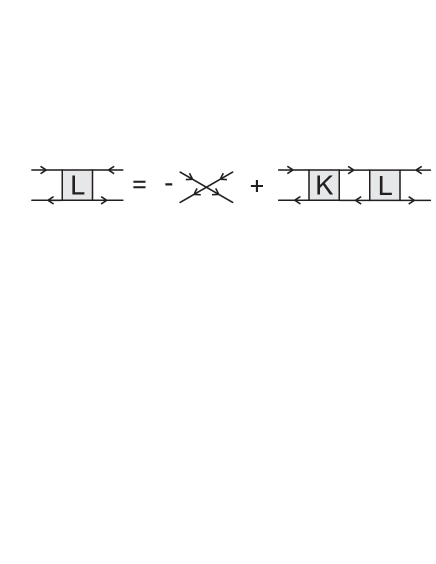
Figure 1: Graphical representation of the Bethe-Salpeter equation for the response function in the ph channel

The response function obeys an integral equation of the form

$$L(13,24)=-g(1,4)g(3,2)$$

$$-i\int{d5d6d7d8\;g(1,5)K(57,68)L(83,74)g(6,2)}\,,$$ (2.5)

where $K$ is an effective two-body interaction. A graphical representation of eq.(II) is given in Fig.1. One should note that the kernel $K$ of the integral equation is the irreducible part of the response function with respect to the particle-hole propagator. We further introduce the vertex function $\widetilde{\tau}$ by

$$L(13,24)=\int{d5d6\;g(1,5)\;\widetilde{\tau}{(53,64)}\;g(6,2)}\,.$$ (2.6)

The corresponding equation follows from eq.(II)

$${\widetilde{\tau}{(13,24)}}=-\delta(1,4)\delta(3,2)$$ (2.7)

$$-i\int{d5d6d7d8\;K(17,28)g(8,5)g(6,7)\widetilde{\tau}(53,64)}\,.$$

In this paper we investigate the excitation energies and transition amplitudes of double closed-shell nuclei. With the time order $t_{3},t_{4}>t_{1},t_{2}$ we insert into the two-particle Green function a complete system of eigenfunctions of the A-particle system between the two particle-hole pairs:

$$g(13,24)=\sum_{n=0}^{\infty}\;g^{0n}(34)g^{n0}(12)\,.$$ (2.8)

with

$$g^{0n}(34)\;=\;-i\left\langle A0\right|T{\left\{{a(3)a^{+}(4)}\right\}}{\left|An\right\rangle}$$ (2.9)

and

$$g^{n0}(12)\;=\;-i\left\langle An\right|T{\left\{{a(1)a^{+}(2)}\right\}}{\left|A0\right\rangle}\,.$$ (2.10)

The spectral representation of the response function eq.(2.4) is also given by eq.(2.8), but the sum begins at $n=1$

$$L(13,24)=\sum_{n=1}^{\infty}\;g^{0n}(34)g^{n0}(12)\,.$$ (2.11)

With the appropriate time-ordering and a Fourier transformation one obtains the spectral representation the response function

$$L_{13,24}=\sum_{n=1}^{\infty}\;\left(\frac{\chi^{n0*}_{12}\chi^{n0}_{43}}{\Omega+E_{n}-i\delta}-\frac{\chi^{n0}_{21}\chi^{n0*}_{34}}{\Omega-E_{n}+i\delta}\right)_{\delta\rightarrow 0^{+}}.\,$$ (2.12)

Here $E_{n}$ are the (exact) energies of the excited states of the A-particle system and

$$\chi^{n0}_{12}=<An|a^{+}_{1}a_{2}|A0>$$ (2.13)

are the corresponding transition matrix elements between the ground state and the excited states of the A-particle system. In the actual calculation we solve the equation for the change of the density in an external field and determine its poles.

II.1 One-particle Green function and the nuclear shell model

In order to solve the equation for the response function and vertex function, respectively, we have to know the one-particle Green functions $g(1,2)$ and the effective two-body interaction $K$. As Landau has shown, one does not need the full information included in $g$, but only the so-called pole part of the one-body Green functions near the Fermi surface. The rest gives rise to a renormalized interaction and effective one-body operators. We first discuss the pole part of the one-body Green function. For that we consider the Dyson equation in coordinate space Migdal67

$$\left({\epsilon-\frac{p^{2}}{2m}}\right)g{\left({\xi_{1},\xi_{2},\epsilon}\right)}$$

$$-\int{d\xi_{3}\;{\Sigma(\xi_{1},\xi_{3},\epsilon)}}\;g(\xi_{3},\xi_{2},\epsilon)=\delta({\xi_{1}}-\xi_{2})\,,$$ (2.14)

where $\xi\equiv{(\bm{r},s)}$ represents space and spin coordinates. In an arbitrary single-particle basis $\widetilde{\varphi}_{\nu}(\xi)$ the Dyson equation has the form

$$\epsilon\;g_{\nu_{1}\nu_{2}}-\sum_{\nu_{3}}\left[\frac{p^{2}}{2m}+\Sigma(\xi_{1},\xi_{3},\epsilon)\right]_{\nu_{1}\nu_{3}}g_{\nu_{3}\nu_{2}}=\delta_{\nu_{1}\nu_{2}}\,.$$ (2.15)

We now chose a special basis $\varphi_{\nu}(\xi)$ that diagonalizes the expression in the brackets

$$\left[\frac{p^{2}}{2m}+\Sigma(\xi_{1},\xi_{3},\epsilon)\right]_{\nu_{1}\nu_{3}}=E_{\nu_{1}}(\epsilon)\delta_{\nu_{1}\nu_{3}}\,.$$ (2.16)

It is obvious that such a basis must depend on the energy $\epsilon$. The one-body Green function becomes diagonal in this basis and can be written as

$$g_{{\nu_{1}}\nu_{2}}=\frac{{\delta}_{\nu_{1}\nu_{2}}}{\epsilon-E_{\nu_{1}}(\epsilon)}\,.$$ (2.17)

Due to Landau’s renormalization procedure one needs the one-particle Green functions only near the dominant poles $\epsilon_{\nu}$, i.e. near the poles, which are the solutions of the equation

$$\epsilon_{\nu}=E_{\nu}(\epsilon_{\nu})$$ (2.18)

and having maximal single-particle strengths (see below). The single-particle energies $\epsilon_{\nu}$ so defined are the quasi-particle energies (in the sense of Landau) for finite systems. In the vicinity of $\epsilon_{\nu}$ we obtain for the one-(quasi)particle Green function

$$g_{\nu_{1}\nu_{2}}(\epsilon)=\frac{\delta_{\nu_{1}\nu_{2}}}{\epsilon-\epsilon_{\nu_{1}}+i\gamma_{\nu_{1}}}\;{\frac{1}{\left(1-{\frac{dE_{\lambda}}{d\epsilon}}\right)}}_{\epsilon=\epsilon_{\nu_{1}}}\,.$$ (2.19)

The residue of $g$ at the pole is called the single-particle strength

$$z_{\nu}={\frac{1}{\left(1-{\frac{dE_{\nu}}{d\epsilon}}\right)}}_{\epsilon=\epsilon_{\nu_{1}}}\,.$$ (2.20)

Within the framework of this method it is easy to derive an equation for the single-particle energies and the single-particle wave functions. To this aim let us omit, for the sake of simplicity, the spin variables and introduce the self-energy in a mixed representation:

$$\Sigma(\bm{R},\bm{k},\epsilon)=\int d\bm{s}\,\Sigma(\bm{R}-{\textstyle\frac{1}{2}}\bm{s},\bm{R}+{\textstyle\frac{1}{2}}\bm{s},\epsilon)\,e^{i\bm{s}\bm{k}}\,,$$ (2.21)

where $\bm{R}={\textstyle\frac{1}{2}}(\bm{r}_{1}+\bm{r}_{2})$, $\bm{s}=\bm{r}_{2}-\bm{r}_{1}$. The local energy approximation (see PS64 ) consists in the replacement of the function $\Sigma(\bm{R},\bm{k},\epsilon)$ by the following ansatz:

$$\Sigma(\bm{R},\bm{k},\epsilon)\simeq\bar{\Sigma}(\bm{R},k^{2}_{F},\epsilon_{F})$$

$$+\,(k^{2}-k^{2}_{F})\left(\partial\bar{\Sigma}(\bm{R},k^{2},\epsilon_{F})/\partial k^{2}\right)_{k^{2}=k^{2}_{F}}$$

$$+\,(\epsilon-\epsilon_{F})\left(\partial\bar{\Sigma}(\bm{R},k^{2}_{F},\epsilon)/\partial\epsilon\right)_{\epsilon=\epsilon_{F}}\,,$$ (2.22)

where $\bar{\Sigma}(\bm{R},k^{2},\epsilon)$ is the average with respect to the angular variables of vector $\bm{k}$,

$$\bar{\Sigma}(\bm{R},k^{2},\epsilon)=\int d\bm{s}\,\Sigma(\bm{R}-{\textstyle\frac{1}{2}}\bm{s},\bm{R}+{\textstyle\frac{1}{2}}\bm{s},\epsilon)\,\frac{\sin(ks)}{ks}$$ (2.23)

and the Fermi energy $\epsilon_{F}$ is related to the Fermi momentum $k_{F}(\bm{r})$ by the formula

$$\frac{\hbar^{2}}{2m}\,k^{2}_{F}(\bm{r})+\bar{\Sigma}(\bm{r},k^{2}_{F}(\bm{r}),\epsilon_{F})=\epsilon_{F}\,.$$ (2.24)

On substituting eq.(II.1) into the Dyson equation (II.1) we come, after a series of transformations, to the following equation for the eigenfunctions:

$$\left[-\bm{\nabla}\frac{\hbar^{2}}{2m^{*}(\bm{r})}\bm{\nabla}+U_{c}(\bm{r})\right]\,\varphi_{\lambda}(\bm{r})=\epsilon_{\lambda}\,\varphi_{\lambda}(\bm{r})\,,$$ (2.25)

where

$$\frac{m}{m^{*}(\bm{r})}=a(\bm{r})\left[1+\frac{2m}{\hbar^{2}}\left(\frac{\partial\bar{\Sigma}(\bm{r},k^{2},\epsilon_{F})}{\partial k^{2}}\right)_{k^{2}=k^{2}_{F}(\bm{r})}\right]\,$$ (2.26)

and

$$a(\bm{r})=\left[1-\left(\frac{\partial\bar{\Sigma}(\bm{r},k^{2}_{F}(\bm{r}),\epsilon)}{\partial\epsilon}\right)_{\epsilon=\epsilon_{F}}\right]^{-1}\,.$$ (2.27)

If we also take the spin degree of freedom into account then, proceeding in the same way, one obtains the following single-particle Hamiltonian:

$$H=-\bm{\nabla}\frac{\hbar^{2}}{2m^{*}(\bm{r})}\bm{\nabla}+U_{c}(\bm{r})$$

$$+{\textstyle\frac{1}{2}}\,[\alpha(\bm{r})\,(\bm{\sigma}\bm{l})+(\bm{\sigma}\bm{l})\,\alpha(\bm{r})]\,.$$ (2.28)

Here $\bm{l}$ is the angular momentum operator. The form of this Hamiltonian follows from the expansion of the self-energy $\Sigma$ about the Fermi energy $\epsilon_{F}$ and the Fermi momentum $p_{F}$, and symmetry arguments. This Hamiltonian agrees with phenomenological shell model Hamiltonians. It is useful to point out Migdal67 that the spin-orbit term follows here from the expansion of the non-locality of $\Sigma$. A certain fraction of the non-locality may be connected with the $\omega$ and $\sigma$ exchange of the bare nucleon-nucleon interaction but certainly not the whole effect, as is assumed in some of the relativistic effective mean field approaches.

II.2 Landau’s renormalization procedure

We now return to the one-particle Green function. With eqs.(2.19 and 2.20) we can separate the one-particle Green function into a singular part and a remainder:

$$g_{\nu_{1}\nu_{2}}(\omega)=\frac{\delta_{\nu_{1}\nu_{2}}z_{\nu_{1}}}{\omega-\epsilon_{\nu_{1}}+i\eta\;sign(\epsilon_{\nu_{1}}-\mu)}\;+\;g^{(r)}_{\nu_{1}\nu_{2}}(\omega)\,,$$ (2.29)

with

$$z_{\nu_{1}}={\left|\left\langle A0\left|a_{\nu_{1}}\right|A+1\;\nu{{}_{1}}\ \right\rangle\right|}^{2}$$

$$\epsilon_{\nu_{1}}=E^{A+1}_{\nu_{1}}-E^{A}_{0}\;\;\;\;for\;\;\epsilon_{\nu_{1}}>\mu$$ (2.30)

$$z_{\nu_{1}}={\left|\left\langle A0\left|a^{+}_{\nu_{1}}\right|A-1\;\nu{{}_{1}}\ \right\rangle\right|}^{2}$$

$$\epsilon_{\nu_{1}}=E^{A}_{0}-E^{A-1}_{\nu_{1}}\;\;\;\;for\;\;\epsilon_{\nu_{1}}<\mu\,,$$ (2.31)

where $\left|A\pm 1\;\nu{{}_{1}}\right\rangle$ denotes an excited state of the $A\pm 1$-particle system. With this ansatz one writes the product of two one-particle Green functions—a quantity that appears in all the integral equations we have derived before—as a singular part $S$ and the remainder $R$, using the ansatz in eq.(2.29)

$$g_{\nu_{1}\nu_{3}}\left(\omega+\frac{1}{2}\Omega\right)g_{\nu_{2}\nu_{4}}\left(\omega-\frac{1}{2}\Omega\right)=$$

$$S_{\nu_{1}\nu_{2}\nu_{3}\nu_{4}}\left(\omega;\Omega\right)+R_{\nu_{1}\nu_{2}\nu_{3}\nu_{4}}\left(\omega;\Omega\right)\,,$$ (2.32)

with

$$S_{\nu_{1}\nu_{2}\nu_{3}\nu_{4}}\left(\omega;\Omega\right)=2\pi iz_{\nu_{3}}z_{\nu_{4}}\delta_{\nu_{1}\nu_{3}}\delta_{\nu_{2}\nu_{4}}$$

$$\times\delta\left(\omega-\frac{\epsilon_{\nu_{3}}+\epsilon_{\nu_{4}}}{2}\right)\;\frac{n_{\nu_{2}}-n_{\nu_{1}}}{\epsilon_{\nu_{2}}-\epsilon_{\nu_{1}}-\Omega}\,.$$ (2.33)

Here $n_{\nu}$ are the quasi-particle occupation numbers ($1$ or $0$) and $\Omega$ is the energy transfer between particle and hole states. Using Landau’s renormalization procedure, one obtains from eq.(2.8) an equation for the renormalized vertex function $\tau$:

$$\tau_{\nu_{1}\nu_{3},\nu_{2}\nu_{4}}\left(\omega,\Omega\right)=\tau^{\omega}_{\nu_{1}\nu_{3},\nu_{2}\nu_{4}}\left(\omega,\Omega\right)+$$

$$\sum_{\nu_{5}\nu_{6}}F^{ph}_{\nu_{1}\nu_{5},\nu_{2}\nu_{6}}\left(\omega,\frac{\epsilon_{\nu_{5}}+\epsilon_{\nu_{6}}}{2},\Omega\right)$$

$$\times\frac{n_{\nu_{5}}-n_{\nu_{6}}}{\epsilon_{\nu_{5}}-\epsilon_{\nu_{6}}-\Omega}\;\tau_{\nu_{5}\nu_{3},\nu_{6}\nu_{4}}\left(\frac{\epsilon_{\nu_{5}}+\epsilon_{\nu_{6}}}{2};\Omega\right)\,.$$ (2.34)

The renormalized vertex is defined as

$$\tau_{\nu_{1}\nu_{3},\nu_{2}\nu_{4}}\left(\omega,\Omega\right)=\sqrt{z_{\nu_{1}}z_{\nu_{2}}}\;\widetilde{\tau}_{\nu_{1}\nu_{3},\nu_{2}\nu_{4}}\left(\omega,\Omega\right)\,.$$ (2.35)

Here only the singular part of the product of the two Green functions appears explicitly, whereas the remainder gives rise to a renormalized effective two-body interaction $F^{ph}$ and a renormalized inhomogeneous term $\tau^{\omega}$. In similar fashion one can renormalize the response function $L$ and obtains

$$L(13,24)=\tau^{\omega}(13,57)\widetilde{L}(57,68)\tau^{\omega}(68,24)$$ (2.36)

$$+\tau^{\omega}(13,57)R(57,24)\,,$$

where $\widetilde{L}$ is the quasi-particle response function

$$\widetilde{L}(13,24)=S(1,2)\tau(1324)\,.$$ (2.37)

II.3 The renormalized equations of the TFFS

As we have seen in section II, the response function includes the transition amplitudes between the ground state and the excited states of an A-particle system. Using the arguments in section II and the projection procedure described in rev77 , one obtains from the renormalized response function in eq.(2.36) and the renormalized vertex function eq.(II.2) an equation for the quasi-particle quasi-hole transition matrix elements

$$\left(\epsilon_{\nu_{1}}-\epsilon_{\nu_{2}}-\Omega\right)\chi^{m}_{\nu_{1}\nu_{2}}=\left(n_{\nu_{1}}-n_{\nu_{2}}\right)\sum_{\nu_{3}\nu_{4}}F^{ph}_{\nu_{1}\nu_{4}\nu_{2}\nu_{3}}\;\chi^{m}_{\nu_{3}\nu_{4}}\,,$$ (2.38)

which are connected with the full ph-transition matrix elements $\chi^{m0}_{\nu_{1}\nu_{2}}$ defined in eq.(2.13) by the relation

$$\chi^{m0}_{\nu_{1}\nu_{2}}=\sum_{\nu_{3}\nu_{4}}\tau^{\omega}_{\nu_{3}\nu_{1}\nu_{4}\nu_{2}}\;\chi^{m}_{\nu_{3}\nu_{4}}\,.$$ (2.39)

The transition matrix element of a one-body operator $Q$ is given by

$$\left\langle Am\right|Q\left|A0\right\rangle\;=\sum_{\nu_{1}\nu_{2}}Q^{\rm eff}_{\nu_{1}\nu_{2}}\;\chi^{m}_{\nu_{1}\nu_{2}}\,,$$ (2.40)

where $Q^{\rm eff}$ is the renormalized one-body operator

$$Q^{\rm eff}_{\nu_{1}\nu_{2}}=\sum_{\nu_{3}\nu_{4}}\tau^{\omega}_{\nu_{1}\nu_{3}\nu_{2}\nu_{4}}Q_{\nu_{3}\nu_{4}}\,.$$ (2.41)

There exist many derivations of the RPA equations (2.38). In all cases the equations have the identical form but the approximations that led to them are quite different. In the present derivation within the many-body Green functions no approximations have been made so far. We arrive, however, at a renormalized ph interaction which, in principle, can be calculated starting from the bare nucleon-nucleon interaction. This, however, is not done in practice. An important result of our derivation concerns the single-particle energies, which are major input data. The quasi-particle energies in the single-particle Green functions (eq.(2.29)) are the experimental single-particle energies of the $\rm A\pm 1$ particle system. In the case of self-consistent calculations this means that one has to choose an interaction that reproduces in mean field approximation the experimental single-particle spectrum of the neighboring nuclei. This point will be discussed again in connection with the extended theory.

From eq.(II.2) one obtains the change of the quasi-particle density in an external field (details are given in Ref.Migdal67 ; rev77 ):

$${\rho}_{\nu_{1}\nu_{2}}(\Omega)=\frac{n_{\nu_{1}}-n_{\nu_{2}}}{\epsilon_{\nu_{1}}-\epsilon_{\nu_{2}}-\Omega}Q^{\rm eff}_{\nu_{1}\nu_{2}}(\Omega)$$

$$-\frac{n_{\nu_{1}}-n_{\nu_{2}}}{\epsilon_{\nu_{1}}-\epsilon_{\nu_{2}}-\Omega}\sum_{\nu_{3}\nu_{4}}F^{ph}_{\nu_{1}\nu_{3}\nu_{2}\nu_{4}}\rho_{\nu_{4}\nu_{3}}(\Omega)\,.$$ (2.42)

The actual calculations presented here have been performed in $\bf{r}$-space because this allows treatment of the continuum in the most efficient way. The corresponding equation takes the form Ka93 ; rev

$$\rho(\bm{r},\Omega)=-\int d^{3}\bm{r}^{\prime}A(\bm{r},\bm{r}^{\prime},\Omega)Q^{\rm eff}(\bm{r}^{\prime},\Omega)$$ (2.43)

$$-\int d^{3}\bm{r}^{\prime}d^{3}\bm{r}^{\prime\prime}A(\bm{r},\bm{r}^{\prime},\Omega)F^{ph}(\bm{r}^{\prime},\bm{r}^{\prime\prime})\rho(\bm{r}^{\prime\prime},\Omega)\,.$$

The poles of the equation are the excitation energies of the A-particle system and $\rho(\bm{r},\Omega)$ at a given pole is the corresponding transition density.

III Extended theory of finite Fermi systems (ETFFS)

As mentioned earlier, the original TFFS allows one to calculate only the centroid energies and total transition strength of giant resonances because the approach is restricted to 1p1h configurations. In order to describe nuclear structure properties in more detail one has to include 2p2h, or even more complex configurations. A theoretical approach that takes into account the complete 2p2h configuration space and a realistic 2p2h interaction is numerically intractable if one uses a realistically large configuration space. For this reason the main approximation in the ETFFS concerns the selection of the most important 2p2h configurations. One knows from experiments, e.g. from the neighboring odd mass nuclei of ²⁰⁸Pb, that the coupling of low-lying collective phonons to the single-particle states gives rise to a fragmentation of the single-particle strength, which is seen in even-even nuclei as a spreading width in the giant resonances.

In the past 15 years an extension of the TFFS that includes, in a consistent microscopic way, the most collective low-lying phonons has been developed by some of us VT89 ; rev ; ka06 (and references therein). Many of these ideas have been developed in the early work by Werner Werner66 and Werner and Emrich Werner70 (see also Refs.rev77 ; KS82 ) and Ref.RW73 . In this way one considers a special class of 2p2h configurations because the phonons are calculated within the conventional (1p1h) TFFS. The phonons give rise to a modification of the particle and hole propagators, the ph interaction and the ground state correlations.

III.1 Some basic relations

In Landau’s theory the self energy $\Sigma$ is irreducible in the one-particle and one-hole channels, respectively, and the kernel $K$ in the integral equation for the response function (see Fig.1) is irreducible in the particle-hole channel. One now introduces a hierarchy of energy dependencies. As one can see from eq.(II.2), the particle-hole propagator introduces a strong dependence on the energy transfer $\Omega$. Compared to this singular behavior, one neglects in Landau’s theory the energy dependence of the ph-interaction. One neglects consistently the energy dependence of the self-energy $\Sigma$ in the Dyson equation (II.1) and considers the quasi-particle and quasi-hole poles only. This approach is of leading order in the energy transfer $\Omega$. In the extended theory, in which phonons are introduced, one considers the next-to-leading order in the energy transfer; i.e. the self energy and the ph interaction become energy dependent. We then write, explicitly,

$$\widetilde{\Sigma}_{\nu}(\epsilon)=\Sigma_{\nu}+{\Sigma}^{ext}_{\nu}(\epsilon)\,;$$ (3.44)

$$\widetilde{F}^{ph}_{\nu_{1}\nu_{3},\nu_{2}\nu_{4}}(\Omega)=F^{ph}_{\nu_{1}\nu_{3},\nu_{2}\nu_{4}}+F^{ph,ext}_{\nu_{1}\nu_{3},\nu_{2}\nu_{4}}(\Omega)\,.$$ (3.45)

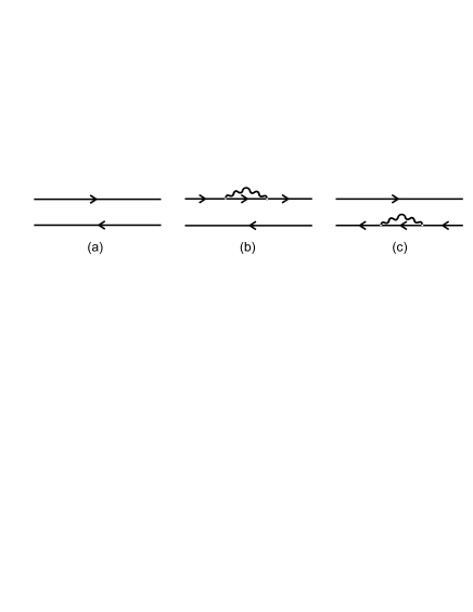
Figure 2: Graphs corresponding to the propagator of (a) the RPA and (b-d) the extended theory. The wavy lines and the thin lines denote the phonons and the single-particle propagators, respectively.

First we discuss the so-called $g^{2}$ approximation Kam84 , which is graphically shown in Fig.2. The upper part of graph (b) gives a correction to the Dyson equation for quasi-particles, which now has the form

$$\left[\epsilon-{\epsilon_{\nu_{1}}}-\sum_{\nu_{2};i}\frac{\left|\gamma^{\nu_{2};i}_{\nu_{1}}\right|^{2}}{\epsilon-\Omega_{i}-\epsilon_{\nu_{2}}}\right]g_{\nu_{1}}^{ext}(\epsilon)=1\,.$$ (3.46)

Here $g_{\nu}^{ext}(\epsilon)$ is the one-quasi-particle Green function in the extended theory and the vertex $\gamma_{\nu}^{\mu;i}$, which couples the quasi-particle state $\nu$ to the core excited configuration $\mu{\otimes}i$, is given by

$$\gamma_{\nu}^{\mu;i}=\sum_{\alpha,\beta}F^{ph}_{\nu\alpha;\mu\beta}\chi^{i}_{\alpha\beta}\,,$$ (3.47)

where $\chi^{i}$ is the RPA wave function of the phonon considered. The corresponding energy-dependent correction for the ph-interaction has the form

$$F^{ph,ext}_{\alpha\mu,\beta\nu}(\Omega,\epsilon,\epsilon^{\prime}) =\sum_{i}\biggl{[}\frac{(\gamma^{\mu;i}_{\beta})^{*}\gamma^{\nu;i}_{\alpha}}{\epsilon-\epsilon^{\prime}+(\Omega_{i}-i\delta)}$$ (3.48)

$$-\frac{(\gamma^{\alpha;i}_{\nu})^{*}\gamma^{\beta;i}_{\mu}}{\epsilon-\epsilon^{\prime}-(\Omega_{i}-i\delta)}\biggr{]}\,.$$

This model has been applied, for example, to M1 resonances in closed shell nuclei KAM89 . In general, the approximation has problems with the so-called second-order poles, which give rise to a distortion of the strength function near these poles. For this reason the model has been extended in several steps: (I) summation of the $g^{2}$ terms KT86 and (II) partial summation of diagrams VT89 , which is called chronological decoupling of diagrams. In the latter case all 1p1h$\otimes$phonon contributions are consistently included and all more complex configurations are excluded—as long as one neglects ground state correlations. The actual formulas, however, include the ground state correlations completely.

In the present analytical approach, as in VT89 , two types of ground state correlations are included: the conventional RPA ground state correlations, which affect the location and the magnitude of the residua of the ph propagators only; and the new type of ground state correlations, caused by the phonons. These correlations are qualitatively different from the conventional RPA correlations because they create new poles in the propagator, which then cause transitions between the 1p1h$\otimes$phonon in the ground state and the excited states. They give rise to a qualitative change of the strength distribution and a change in the sum rules for the moments of the strength function. In the present numerical application we only included the conventional RPA correlations. Calculations which include the complete ground state correlations are in progress.

As in the TFFS, the energy dependence of the generalized propagator, $A^{ext}$, is much stronger than that of the generalized ph interaction, as the next-to-leading order energy dependence is removed from the interaction and explicitly taken into account in the generalized propagator. Therefore one considers explicitly only the energy dependence of the propagator and neglects the energy dependence of the ph interaction. The interaction is parameterized as before, although the corresponding parameters may differ from the previous ones. The final equation for the change of the quasi-particle density in an external field has a form identical to that in the TFFS (eq.(2.43)):

$${\widetilde{\rho}^{ext}(\bm{r},\Omega)=-\int d^{3}\bm{r}^{\prime}A^{ext}(\bm{r},\bm{r}^{\prime},\Omega)}Q^{eff}(\bm{r}^{\prime},\Omega)$$ (3.49)

$${-\int d^{3}\bm{r}^{\prime}d^{3}\bm{r}^{\prime\prime}A^{ext}(\bm{r},\bm{r}^{\prime},\Omega)}F^{ph,}(\bm{r}^{\prime},\bm{r}^{\prime\prime})\widetilde{\rho}^{ext}(\bm{r}^{\prime\prime},\Omega)\,.$$

The analytic form of the generalized propagator can be found in Ref. rev .

In the following we investigate, within the continuum random phase approximation (CRPA) and the ETFFS, electric dipole states in ²⁰⁸Pb. The strength distributions for isovector as well as isoscalar transitions are shown. The single-particle continuum has been included at the RPA level where it is taken into account correctly within our Green function technique in the coordinate representation. For details see rev . In our approach we consider therefore the three mechanisms that create the width of giant resonance, namely (I) the Landau damping ((Q)RPA configurations), (II) the escape width (the single-particle continuum) and (III) the spreading width (phonon coupling, or complex configurations). As in all our previous calculations within the ETFFS, we include the most collective low-lying phonons. These phonons have been microscopically calculated within the RPA. In the present and in our previous calculations we used the procedure developed in kl98 to obtain the energy of the spurious E1 state to be exactly equal to zero without having to use the procedure of fitting force parameters.

III.2 Single-particle basis

Lπ	energies [MeV]
$2^{+}$	4.09 6.44
$3^{-}$	2.61
$4^{+}$	4.32 5.44 6.00
$5^{-}$	3.20 3.66 5.29 6.14 7.22
$6^{+}$	4.42 5.21
$7^{-}$	4.04 4.69 5.03 5.66 6.33 7.17
$8^{+}$	4.61 4.99 5.22 6.23 6.43

Table 1: Phonons used in the ETFFS calculation

We have seen that in the conventional TFFS Landau’s quasi-particle are the single-particle states of the neighboring odd mass nuclei. Therefore one has to use as input data in the corresponding equation for the excited states of the even nuclei (renormalized RPA) the experimental single-particle energies. These single-particle energies include obviously the effect of the coupling to more complicated configurations e.g. phonons. In the actual calculation within the extended theory we consider about twenty low-lying phonons explicitly and for that reason one has first to determine bare single-particle energies that do not include the coupling to those phonons. If we couple the corresponding phonons to the bare single-particle states we reproduce the original quasi-particle energies. In order to obtain the new refined single-particle basis $\widetilde{\epsilon}_{\nu}$ one has to solve eq.(3.50), which can be obtain from eq.(3.46):

$$\widetilde{\epsilon}_{\nu_{1}}=\epsilon_{\nu_{1}}-\sum_{\nu_{2};i}\frac{\left|\gamma^{\nu_{2};i}_{\nu_{1}}\right|^{2}}{\epsilon_{\nu_{1}}-\Omega_{i}-\widetilde{\epsilon}_{\nu_{2}}}\,.$$ (3.50)

Equation ( 3.50) has been first derived by Ring and Werner RW73 . It has been applied to the calculation of the fragmentation of the single particle strength in the neighboring odd mass nuclei of ${}^{208}Pb$ RW73 and the high-spin states in ${}^{208}Pb$ Ref. Krew80 .

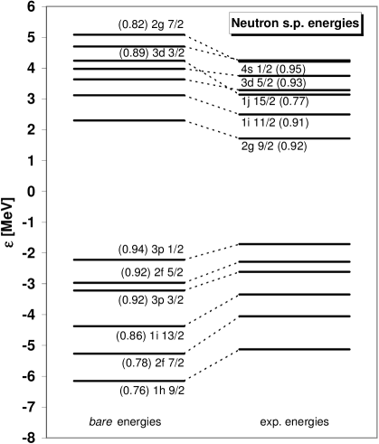
Figure 3: Neutron single-particle energies in ²⁰⁸Pb. Here we compare the experimental values with the bare single-particle energies which were obtained from eq.(3.50). The values in parentheses are the single particle strengths.

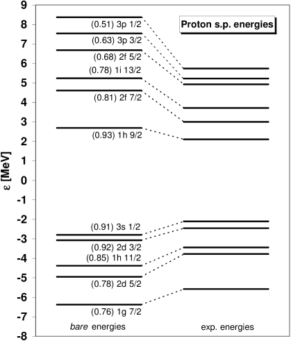
Figure 4: Same as in Fig. 3 for the proton single-particle energies in ²⁰⁸Pb

.

The phonons that are explicitly considered in the present calculation are given in Table 1. In Figs. 3 and 4 the bare single-particle spectrum for protons and neutrons are shown and compared with the experimental spectrum. The energy shift due to the coupling to the phonons is nearly twice as large for the protons as for the neutrons. In addition, one obtains a fragmentation of the single-particle strength. The corresponding values are also given in Figs. 3 and 4. Here we point out that, in addition to the phonon coupling, the short range correlations in the G-matrix also reduce in a uniform way the single-particle strength. This part of the reduction is taken care of by the renormalization procedure in section II. The bare energies may be identified with the mean energies that one obtains within a self-consistent approach. From the present calculation one observes that the (in general) too large spreading of the self-consistent single-particle spectra compared with the experimental ones would be reduced on the average for the neutrons by about 1 MeV and for the protons by 1.5 MeV with relatively large fluctuations. If one solves equation (3.50) with the corresponding mean field solutions one obtains the dressed single-particle energies that should agree (from our point of view) with the experimental spectrum. The number of phonons can be restricted to the most collective ones because they are the most important ones for the width of the giant resonances. They also influence the different single-particle states in an individual manner. If we increase the number of phonons one only obtains an overall shift that is equivalent to a change in the effective mass. We conclude that for a given set of phonons one has to chose an effective interaction with the appropriate effective mass and spin orbit interaction. We return to this question in the final discussion.

III.3 The residual particle-hole interaction

As in our previous calculations we used the effective particle-hole Landau-Migdal interaction

$$F(\bm{r},\bm{r^{\prime}})=C_{0}\left[f(r)+f^{\prime}(r)\bm{\tau}_{1}\cdot\bm{\tau_{2}}\right.$$

$$+\left.(g+g^{\prime}\bm{\tau_{1}}\cdot\bm{\tau_{2}})\bm{\sigma_{1}}\cdot\bm{\sigma_{2}}\right]\;\delta(\bm{r}-\bm{r^{\prime}})$$ (3.51)

with the conventional interpolation formula, for example, for the parameter $f$,

$$f(r)=f_{ex}+(f_{in}-f_{ex})\rho_{0}(r)/\rho_{0}(0)$$ (3.52)

and similarly for the other $r$-dependent parameter $f^{\prime}(r)$. Here $\rho_{0}(r)$ is the density distribution of the ground state of the nucleus under consideration and $f_{in}$ and $f_{ex}$ are the force parameters inside and outside of the nucleus. The standard values of the parameters, which have been used for all the nuclei under consideration rev , are:

$$f_{in}=-0.002,\;f_{ex}=-1.35,\;f_{ex}^{\prime}=2.30,\;f_{in}^{\prime}=0.76,$$

$$g_{in}=g_{ex}=0.05,\;g^{\prime}_{in}=g^{\prime}_{ex}=0.96.$$ (3.53)

The parameters are given in units of $C_{0}=300\;{\rm MeVfm^{3}}$. For the nuclear density $\rho_{0}(r)$ in the interpolation formula we chose the theoretical ground state density distribution of the corresponding nucleus,

$$\rho_{0}(r)=\sum_{\epsilon_{i}\leq\epsilon_{F}}\frac{1}{4\pi}(2j_{i}+1)R^{2}_{i}(r)\,.$$ (3.54)

Here $R_{i}(r)$ are the single-particle radial wave functions of the Woods-Saxon single-particle model. This is more consistent than the previously used phenomenological Fermi distribution. For that reason we readjusted in the present calculation $f_{ex}$ to reproduce the breathing mode and obtained the value of $f_{ex}$ = -1.35. For other details of the calculations, see Ref.rev ; GS06 .

IV Low-lying electric dipole strength

IV.1 The isovector case

The giant electric dipole resonance (GDR) is one of the most collective states in nuclei. It exhausts a major part of the energy-weighted sum rule; the excitation energy is a smooth function of the mass number; and the form of the GDR changes only little from nucleus to nucleus. Phenomenological collective models describe well the A-dependence of the energy and the strength with only a few parameters. In microscopic models these collective states are coherent superpositions of many particle-hole states.

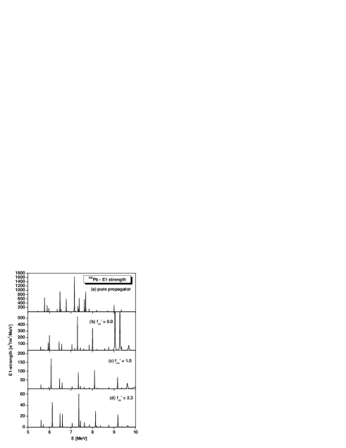
Figure 5: Electromagnetic E1 strength distribution calculated within the conventional 1p1h RPA. In (a) we show the uncorrelated ph-matrix elements. In (b) we used our universal isoscalar interaction and the spurious state has been removed. For the results shown in (c) a reduced isovector force has been used, while (d) shows the results with the full interaction.

The theoretical results of such models for the mean energy and the total strength agree, in general, very well with the data. The strength distribution, however, is reproduced by only a few very involved models, such as the ETFFS considered here.

Here we first investigate the question whether the pygmy dipole resonances (PDR) are like the GDR collective states in the microscopic definition. That is, are they coherent superpositions of many particle-hole states? In order to answer this question we performed a series of calculations within the continuum RPA in which we varied the particle-hole interaction.

In Fig.5a the dipole distribution for the electromagnetic $E1$-operator is plotted, where the particle-hole interaction is zero; i.e. the figure shows pure proton and neutron ph-matrix elements. The largest matrix elements are the ones between the ph states with the largest angular momenta that differ by one unit—the stretched configurations. The state at $E\approx$6.5 MeV is the neutron $(1j_{15/2})(1i_{13/2})^{-1}$ configuration and the states at $E\approx$ 7.15 MeV and $E\approx$ 7.70 MeV are the proton configurations $(1i_{13/2})(1h_{11/2})^{-1}$ and $(1h_{9/2})(1g_{7/2})^{-1}$. The three largest transitions exhaust about 40% of the total strength. Here, we have to bear in mind that the transitions shown also include spurious components that give rise to the spurious isoscalar state at zero energy. This state corresponds to the translation of the whole nucleus. For that reason one has to remove the spurious components in each of the particle-hole configurations. The method developed in Ref. kl98 is used that brings the spurious state exactly to zero energy and removes completely the spurious strength in all excited states.

In Fig.5b-d the electromagnetic dipole strength, from which the spurious strength has been removed, is shown.

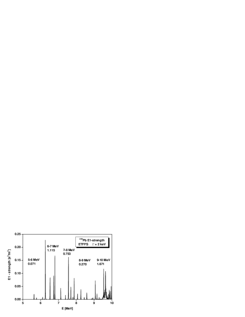
Figure 6: Integrated electromagnetic E1 strength calculated within the ETFFS. These results should be compared with the distribution shown in Fig.5d. Note that the strength in the present figure is integrated over the smearing width, given in $\rm e^{2}fm^{2}$.

To demonstrate the effect of the repulsive isovector interaction we have chosen three different values for the isovector force parameter $f^{\prime}_{ex}$. The isoscalar ph interaction is the same for all three cases. It reproduces the breathing mode, which is later shown in Fig.20. If we compare the completely uncorrelated strength distribution in Fig.5a with the results in Fig.5b, where the spurious components are removed but the isovector force parameter $f^{\prime}_{ex}=0$, one observes an appreciable shift of the B(E1) strength to higher energies. We notice thereby that if one removes the spurious strength one has to introduce correlations that give rise to this redistribution of the strength. With setting the isovector interaction to zero, most of the B(E1) strength (87%) lies below 10 MeV. If we increase the isovector interaction parameter to $f^{\prime}_{ex}=1.0$ (Fig.5c), which is about half of the force parameter that reproduces the experimental data of the GDR, the dipole strength below 10 MeV is reduced to $11\%$.

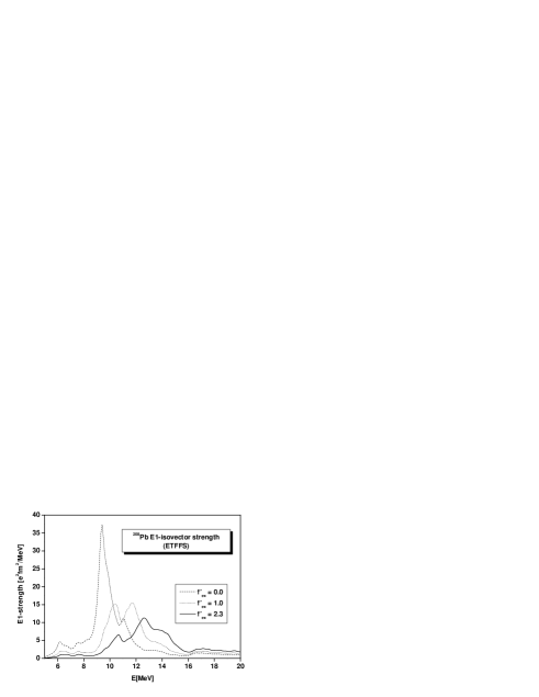
Figure 7: Electromagnetic E1 strength from 5 to 20 MeV calculated in our extended theory. The thick line indicates the final result whereas the other lines are the results of calculations where the isovector force parameter has been varied as indicated in the figure.

Finally, in Fig.5d, where we use our conventional force parameter (which reproduces nearly quantitatively the experimental data of the GDR), only $5.2\%$ of the strength remains below 10 MeV. We observe that the major part of the E1 strength is shifted into the GDR region, where it creates a very collective resonance—in agreement with the data.

Within our model, in the electromagnetic E1 strength up to 9 MeV, which is the region of the pygmy resonance, we do not find one single state in which most of the low-lying strength is concentrated, but we find already in the 1p1h RPA several states whose energies are essentially unchanged compared with the $f^{\prime}_{ex}=0$ case. The E1 strength, however, is reduced by a factor of 10 due to the strongly repulsive isovector force, which shifts the strength into the GDR region and produces a collective resonance. Such a behavior is expected from the schematic model of Brown and Bolsterli GEB .

In Fig.6 we present the results of the ETFFS calculation where, in addition to the single-particle continuum, the effect of the phonons is also included. The phonons that we consider are given in Table 1. The result in Fig.6 should be compared with the results in Fig.5d. One observes a further fragmentation of the strength and a small shift of the two strongest states to higher energies. Whereas the calculated strength distribution between 7 and 8 MeV is in good agreement with the data, we obtain too little strength below 6 MeV and too much between 6-7 MeV as compared with the present data. A shift of the two neutron states $1j_{15/2}$ and $(1i_{13/2})^{-1}$ improves the agreement between theory and experiment.

In Fig.7 the electromagnetic E1 strength distribution calculated within the ETFFS is shown up to 20 MeV with a smearing parameter $\Delta$ = 250 keV and three different $f^{\prime}_{ex}$ parameters. It is interesting to see how the strength is shifted to higher energies with increasing interaction strength. For our conventional value $f^{\prime}_{ex}$ = 2.30 the theoretical distribution in the GDR region agrees quantitatively with the experimental data. In connection with the previous discussion, the energy range between 6-8 MeV is of special interest. With no isovector interaction, but the spurious components removed, one obtains some concentration of strength around 6.2 MeV and 7.5 MeV. The latter is considered as the PDR region. With increasing isovector force this strength is reduced. For the full force the reduction is a factor of 5 compared to $f^{\prime}_{ex}=0$. This behavior is just the opposite of a collective structure, where with increasing force the collectivity is enhanced.

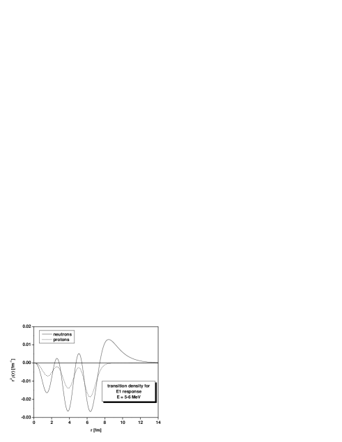
Figure 8: Summed transition densities for the electric dipole response shown in Fig.6 from 5 to 6 MeV

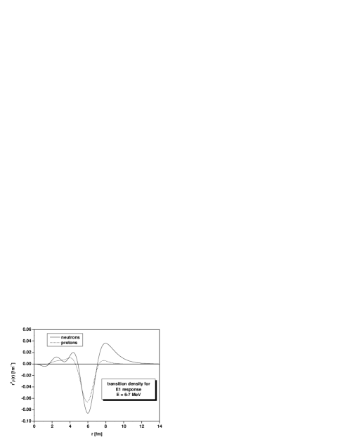
Figure 9: Summed transition densities for the electric dipole response shown in Fig.6 from 6 to 7 MeV

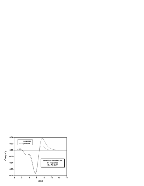
Figure 10: Summed transition densities for the electric dipole response shown in Fig.6 from 7 to 8 MeV

In Figs.8-10 the transition densities between 5-6 MeV, 6-7 MeV and 7-8 MeV of the electric dipole response are plotted for transitions shown in Fig.6. In all three cases the protons and neutrons are in phase, which indicates strong isoscalar components. This at-first-glance surprising behavior has also been found by other authors. It can be understood immediately in our microscopic model. As discussed in the next section, the isoscalar force is attractive and gives rise to a collective structure around 22 MeV. Due to this attractive force, some of the high-lying strength couples also to the low-lying states, whereas the strong repulsive isovector force simultaneously shifts the isovector strength from these configurations into the GDR region. We demonstrate this behavior in Figs.12-14 where the transition densities are plotted for the same energy ranges but with the force parameters $f^{\prime}_{ex}$ set to zero. As the isovector force is zero, the isovector strength remains in the low energy region, which can be clearly seen in the transition densities.

IV.2 The isoscalar case

As mentioned earlier, for the electric isoscalar dipole states we have a special situation because the lowest isoscalar resonance is the spurious state corresponding to the translation of the whole nucleus. In self-consistent calculations this state appears (at least in principle) at zero energy and carries all the spurious strength.

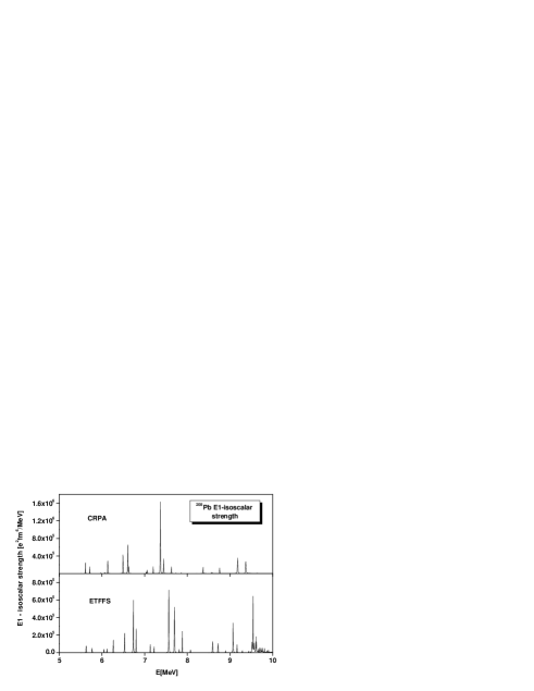
Figure 11: E1 isoscalar strength distribution in ²⁰⁸Pb from 5-10 MeV for the transition operator $(r^{3}-5/3\langle r^{2}\rangle r)Y_{1,\mu}$. Here we compare the results derived from the CRPA with the results obtained with the extended theory.

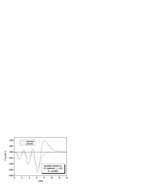
Figure 12: Summed transition densities from 5 to 6 MeV with the isovector force parameter $f^{\prime}_{ex}=0$

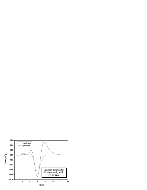
Figure 13: Summed transition densities from 6 to 7 MeV with the isovector force parameter $f^{\prime}_{ex}=0$

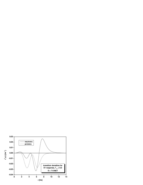
Figure 14: Summed transition densities from 7 to 8 MeV with the isovector force parameter $f^{\prime}_{ex}=0$

In the Landau-Migdal approaches the spurious state has to be removed explicitly. Here we use the procedure developed in Ref.kl98 to obtain the energy of the spurious E1 state exactly at zero energy, with no spurious components in the excited state. As the isoscalar electric dipole strength distribution depends on the isoscalar parameter $f$, we test the force by calculating the isoscalar monopole resonance—the breathing mode. With our universal value of $f_{ex}=-1.35$ we reproduce the mean energy as well as the width of the resonance (see the next section). In Fig.11 the results of our calculation for the isoscalar dipole operator $(r^{3}-5/3\langle r^{2}\rangle r)Y_{1,\mu}$ up to 10 MeV are presented. There we compare the CRPA with the ETFFS results. In the CRPA we obtain one strong state near 7.4 MeV and several somewhat weaker states at lower energies. Due to the phonon coupling the strength of the strongest state is fragmented and shifted to slightly higher energies. Those isoscalar states have been investigated experimentally with the $(\alpha,\alpha^{\prime},\gamma_{0})$ reaction. So far the experimental data from ²⁰⁸Pb are not given in the form of cross sections but only in counts hvw01 . The data show a very strong signal at about 5.6 MeV and a somewhat weaker signal around 6.7 MeV. As the isoscalar strength distribution in Fig.11 is calculated with the operator $(r^{3}-5/3\langle r^{2}\rangle r)Y_{1,\mu}$, a comparison with these data is not directly possible because the $(\alpha,\alpha^{\prime})$ reaction is sensitive to the tails of the isoscalar distributions and the $\gamma_{0}$ is proportional the isovector admixture. Unfortunately, analyzing programs in which microscopic transition densities can be used do not yet exist Zil06 . The transition densities shown previously are the same for the isoscalar and isovector case. Only the transition strength is different because the corresponding operators weight the transition densities differently.

V High-lying electric dipole strength

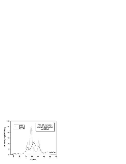
Figure 15: E1 isovector strength from 5 to 20 MeV. We compare here the results of the continuum RPA with the extended theory the width and the mean energy of the latter agree quantitatively with the experimental results.

Figure 16: Transition density of the isovector giant dipole resonance

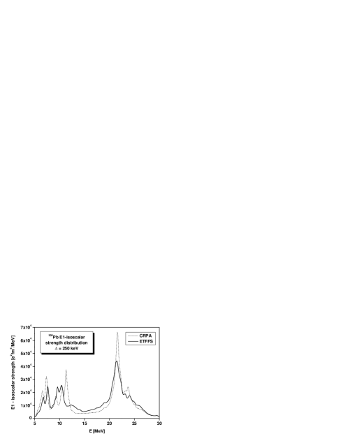
Figure 17: Isoscalar E1 strength from 5 to 30 MeV calculated with a smearing parameter $\Delta$ = 250 keV

Figure 18: Transition density of the isoscalar giant dipole resonance

Figure 19: Isoscalar E1 strength calculated with a smearing parameter $\Delta$= 3 MeV. Note: The larger smearing parameter is justified only for the high-lying ($\geq$15 MeV) part of the resonance.

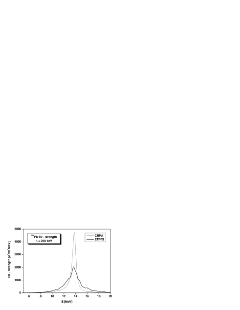
Figure 20: Isoscalar E0 strength from 5 to 20 MeV calculated in the continuum RPA and the extended theory. The mean energy and width of the latter agrees with the data.

Figure 21: Transition density of the breathing mode

The GDR was calculated with our universal parameters given in eq.(III.3) and the result is shown in Fig.15. The mean energy and the width of the resonance agree with the data within the error bars. The escape and spreading widths are included in our microscopic model. In addition, we consider a smearing parameter $\Delta$ = 250 keV , which corrects for more complex configurations that have not be considered in our approach. Here we point out again that the low-lying and high-lying E1 strength is calculated within the same model with exactly the same single-particle energies and force parameters. This differs from some self-consistent approaches in which the single-particle spectrum is modified in order to fit the low-lying spectrum e.g. HL02 .

In Fig.16 the corresponding transition density is plotted. It is surface-peaked and protons and neutrons are out of phase. As we have 50% more neutrons than protons, the neutron density has not only a stronger and longer tail than the proton density, but it is also peaked further out. For that reason we also have some admixture of isoscalar E1 strength—even in the isovector giant dipole region. The form of the transition density agrees with surface-peaked phenomenological models.

In Fig.17 the theoretical isoscalar E1 response from 5-30 MeV is plotted. One realizes that, in addition to the low-lying strength, we obtain a strong collective structure above 20 MeV, which represents the isoscalar electric dipole resonance. The mean energy of the resonance is $\widetilde{E}_{th}$ = 22.1 MeV and the width $\Gamma_{th}$ = 3.8 MeV if we chose a smearing parameter $\Delta$ = 250 keV. The deep-lying holes contribute a major part to the high-lying E1-strength. These holes are several MeV broad. These widths are not included in the calculation shown in Fig.17 where we used a smearing parameter of $\Delta$ = 250 keV. In order to correct for these widths we performed a calculation with $\Delta$ = 3 MeV, the corresponding result is shown in Fig.19. The theoretical results can be compared with a recent $(\alpha,\alpha^{\prime})$ experiment Uchida03 , which obtained $\widetilde{E}_{exp}$ = 22.5-23.0 MeV and a width $\Gamma_{exp}\approx$ 10 MeV. The corresponding transition density is given in Fig.18. It has the form of a compression mode and for that reason we have shown—finally—in Figs.20 and 21 the isoscalar monopole strength and the corresponding transition density. These calculations are performed for purpose of consistency because the isoscalar monopole and isoscalar dipole depend both on the isoscalar parameters $f$ and have, in addition, a very similar structure, as can be seen in the transition densities. In the monopole case the radial integral over the transition density has to be zero; in the electric dipole case the transition density multiplied by the radial coordinate $r$ must vanish.

VI Discussion

The center of our investigations has been the origin and the structure of the pygmy resonances. We have chosen in ²⁰⁸Pb a nucleus with an excess of 44 neutrons, which means that we have $50\%$ more neutrons than protons. The structure of this doubly-magic nucleus, as well as of the neighboring odd mass nuclei, is well known and all microscopic models and microscopic theories—self-consistent ones and Landau-Migdal —work best for this case.

Our calculation shows, first of all, that we obtain isovector as well as isoscalar electric dipole states below 10 MeV. This is obvious, as the ph-interaction has isoscalar as well as isovector components. Here we point out that all the spurious components are removed; i.e. the expectation value of the translation operator $rY_{1\mu}$ in all the excited states is negligibly small. The isoscalar strength is due to the $3\hbar\omega$ and higher ph components. In the present Landau-Migdal approach one is able to remove the spurious strength without performing a full RPA calculation, as must be done in self-consistent approaches. Here, the force parameters can be varied independently. This allows one to investigate the influence of the isovector interaction on the low-lying isovector dipole strength in detail.

We have shown in Figs.5 and 7 that if one starts with the experimental single-particle energies, then with increasing isovector force the isovector dipole strength is shifted to higher energies and one is finally left with a small fraction of the sum rule in a few states that are only slightly shifted with respect to the unperturbed ph energies. There is no indication in the present model of a low-lying collective state that is built up by the isovector interaction. The theoretical electromagnetic strength below 8 MeV is 1.94 $[e^{2}fm^{2}]$ compared with the experimental strength of 1.32 $[e^{2}fm^{2}]$. The distribution of the theoretical strength agrees in the range between 7-8 MeV with the current data. The calculated strength between 6-7 MeV, however, is too large and the strength below 6 MeV too small compared with the experimental values. On the other hand, the width and the mean energy of the GDR is reproduced quantitatively in our model.

It is obvious that if one changes the single-particle spectrum one is always able to improve the agreement with the data. In the present calculation we only consider the lowest order in the expansion of the Migdal interaction, as is done in nearly all calculations. The next-to-leading order in Migdal’s interaction depends on the momenta through $\bm{p}\cdot\bm{p^{\prime}}$, with the isoscalar force parameter $f_{1}$ and the isovector force parameter $f^{\prime}_{1}$. The sign and magnitude of the two parameters can be estimated from the effective mass of the nucleus and the orbital part of the effective magnetic operator rev77 . From this consideration it follows that both parameters are negative, with the $f^{\prime}_{1}$ parameter slightly smaller in magnitude. These parameters would give rise to an attractive velocity dependent isoscalar and isovector ph interaction. A small effective mass, as is used in relativistic RPA calculations, would increase the magnitude of both parameters. A strong isovector, velocity dependent force could be the explanation of the collective states with large vorticities that are found in relativistic RPA calculations ring05 . In this approach two phonon states will give rise to a fragmentation that should explain the E1 data between 5 and 9 MeV. Unfortunately, the lowest two phonon states are at 6.7 and 6.9 MeV, whereas the lowest experimental E1-states are more then one MeV lower. We therefore consider the present result, where the E1 strength between 5.5-9 MeV lies essentially at the unperturbed ph-energies and the major part of the isovector E1 strength is shifted into the GDR, to be the more physical one. Moreover, a collective phenomenon has not been found in self-consistent calculations in which one starts with effective forces of the Skyrme type. The next-to-leading order in Migdal’s interaction ($f_{1}$,$f^{\prime}_{1}$) will lead to some redistribution of the low-lying strength which may improve the agreement with the data below 7 MeV. Such calculations are in progress.

VII Consequences for self-consistent calculations

The present calculation is not self-consistent in the sense that one starts with an effective Lagrangian (or Hamiltonian), the numerous parameters of which are, in general, adjusted to gross properties of nuclei and can be used for all nuclei. These parameters cannot be determined in a unique way and therefore there exist numerous sets of parameters that reproduce the gross properties equally well, but give quite different results for excited states. If we consider, as a specific example, effective forces of the Skyrme type, we find parameterizations that, for example, give rise to effective masses from ${m^{*}}/{m}$ = .6 to ${m^{*}}/{m}$ = 1. For nuclear structure calculations the effective mass is of special importance because the spacing of the single-particle spectrum is inversely proportional to it; a smaller $m^{*}/m$ expands the single-particle spectrum and a larger one compresses the spectrum. The experimental single-particle spectra in the neighboring odd mass nuclei of ²⁰⁸Pb correspond to an effective mass of roughly one, whereas for medium mass nuclei it is smaller then one. If one describes the spectrum in the odd mass nuclei correctly one simultaneously reproduces the non-collective states in ²⁰⁸Pb. The collective states, on the other hand, depend not only on the ph-spectrum but also on the residual ph interaction. It seems always possible to find, under the numerous sets of Skyrme parameters, one set that reproduces the collective states in which one is interested, whereas the non-collective ones deviate from the data by several MeV.

In our calculations we investigated simultaneously the E1 spectrum between 5-8 MeV and the high-lying spectrum. Our calculations show that the E1 spectrum below 8 MeV is very similar to the unperturbed experimental ph spectrum, whereas the high-lying collective states depends sensitively on the (universal) Migdal parameters. This is not an exception; rather, it is the general experience. In the low energy spectrum of ²⁰⁸Pb one finds some collective states with natural parity that are collective (e.g. $3^{-},5^{-},2^{+}$ etc.) but the majority of the states—especially the low-lying unnatural ones—are energetically at the experimental ph energies. Therefore, if one is looking for a unified description of the structure of even-even nuclei, one has also to consider the spectra of the neighboring odd mass nuclei.

VIII Summary

The extended theory of finite Fermi systems has been applied to the low-lying and high-lying E1 spectrum of ²⁰⁸Pb as an example of a neutron-rich nucleus. In the present approach the low-lying electromagnetic E1 spectrum is non-collective in the sense that the major part of the strength is not concentrated in one single state. The strength is rather distributed over several states which are close to unperturbed ph energies and we find in the low-lying E1 states strong isoscalar admixtures. The theoretical results for the GDR as well as the breathing mode agree quantitatively with the data. We also find in our calculation a well-localized isoscalar E1 resonance at 22.2 MeV, with a width of 9.3 MeV. This resonance has been detected in $(\alpha,\alpha^{\prime})$ scattering.

From the present investigation one may draw important conclusions concerning self-consistent calculations. We have seen that the inclusion of the phonons gives rise to a shift of the single-particle spectrum of about 1 MeV for neutrons and nearly 2 MeV for protons. In the present extended theory one has to determine bare single-particle energies that give the experimental ones if one includes the phonons. Self-consistent approaches determine the bare spectrum that we need to use as input in our extended theory. One therefore has to chose a parametrization of the effective intercation that reproduces —if one includes the phonons—the experimental spectrum. From this point of view, self-consistent calculations for excited states at the level of the 1p1h RPA are not appropriate.

IX Acknowledgment

We thank Sergey Kamerdzhiev for many useful comments. One of us (JS) thanks Stanislaw Drożdż for many discussions and the Foundation for Polish Science for financial support through the Alexander von Humboldt Honorary Research Fellowship. The work was partly supported by the DFG and RFBR grants Nos.GZ:432RUS113/806/0-1 and 05-02-04005 and by the INTAS grand No.03-54-6545.

References

- (1) R.Palit, P.Adrich, T.Aumann, et al., Nucl.Phys. A731 (2004) 235.
- (2) U.Kneisl, H.H.Pilz and A.Zilges, Progr.Part.Nucl.Phys. 37 (1996) 349.
- (3) T.Hartmann, J.Enders, P.Mohr, et al., Phys.Rev. C65 (2002) 034301.
- (4) T.Hartmann et al., Phys.Rev.Lett. 93 (2004) 192501.
- (5) R.M.Laszewski, P.Rullhusen, S.D.Hoblit and S.F.LeBrun, Phys.Rev.Lett. 54 (1985) 530.
- (6) M.N.Harakeh and A.van der Woude, Giant Resonances (Clarendon Press, Oxford, 2001).
- (7) A.Zilges, private communication and D.Savran et al., Phys.Rev.Lett. (in press).
- (8) Y.Suzuki, K.Ikeda and H.Sato, Progr.Theor.Phys. 83 (1990) 180.
- (9) P.Van Isacker, M.A.Nagarajan and D.D.Warner, Phys.Rev. C45 (1992) R13
- (10) S.Typel and G.Baur, Phys.Rev.Lett. 93 (2004) 142502.
- (11) D.Vretenar, A.V.Afanasjev, G.A.Lalazissis and P.Ring, Phys.Rep. 409 (2005) 101.
- (12) S.Goriely, E.Khan, Nucl.Phys. A706 (2002) 217.
- (13) S.Krewald and J. Speth, Phys.Rev.Lett. 45 (1980) 458.
- (14) G.E.Brown, Rev.Mod.Phys. 43 (1971) 1.
- (15) V.G.Soloviev, Theory of Complex Nuclei (Pergamon Press, Oxford, 1976) [Russ. original, Nauka, 1971].
- (16) V.G.Soloviev, Theory of Atomic Nuclei: Quasiparticles and Phonons (Institute of Physics , Bristol and Philadelphia, USA, 1992).
- (17) S.Kamerdzhiev and V.N.Tkachev, Phys.Lett. B142 (1984) 22.
- (18) V.I.Tselyaev, Sov.J.Nucl.Phys. 50 (1989) 780.
- (19) S.Kamerdzhiev, J.Speth and G.Tertychny, Phys.Rep. 393 (2004) 1.
- (20) N.Tsoneva, H.Lenske, Ch.Stoyanov, Phys. Lett. B 586 (2004) 213; Nucl.Phys. A731 (2004) 273.
- (21) D.Sarchi, P.F.Bortignon, G.Colo, Phys.Lett. B601 (2004) 27.
- (22) A.B.Migdal: Theory of Finite Fermi Systems and Application to Atomic Nuclei (New York:Wiley) 1967.
- (23) J.Speth, E.Werner and W.Wild, Phys.Rep. 33 (1977) 127.
- (24) F.Grümmer and J.Speth, J.Phys. G: Nucl.Part.Phys. 32 (2006) R193.
- (25) S.Kamerdzhiev, J.Speth, G.Tertychny and V.I.Tselyaev, Nucl.Phys. A555 (1993) 90.
- (26) S.Kamerdzhiev, Phys.At.Nucl. 69( 2006) 1143.
- (27) E.Werner, Z.Physik 191 (1966) 381.
- (28) E.Werner and K.Emrich, Z.Physik 236 (1970) 454.
- (29) V.Khodel and E.Saperstein, Phys.Rep. 92 (1982) 183.
- (30) P.Ring and E.Werner Nucl.Phys. A211 (1973) 198.
- (31) S.Kamerdzhiev and V.N.Tkachev, Z.Physik A344 (1989) 19.
- (32) S.Kamerdzhiev and V.I.Tselyaev, Sov.J.Nucl.Phys.44 (1986) 214.
- (33) S.Kamerdzhiev, R.J.Liotta, E.Litvinova and V.Tselyaev, Phys.Rev. C58 (1998) 172.
- (34) S.Kamerdzhiev, J.Speth and G.Tertychny, Nucl.Phys. A624 (1997) 328.
- (35) V.I.Tselyaev, Bull.Rus.Acad.Sci.Phys. 64 (2000) 434.
- (36) G.E.Brown and M.Bolsterli, Phys.Rev.Lett. 3 (1959) 472.
- (37) N.Ryezayeva et al., Phys.Rev.Lett. 89 (2002) 272502.
- (38) M.Uchida et al., Phys.Lett. B557 (2003) 12.
- (39) F.G.Perey and D.S.Saxon, Phys.Lett. 10 (1964) 107.