Equation of State for Hot and Dense Matter: $\sigma$-$\omega$-$\rho$ Model with Scaled Hadron Masses and Couplings

Abstract

The proposed earlier relativistic mean-field model with hadron masses and coupling constants depending on the $\sigma$-meson field is generalized to finite temperatures. Within this approach we simulate the in-medium behavior of the hadron masses motivated by the Brown-Rho scaling. The high-lying baryon resonances and boson excitations as well as excitations of the $\sigma$, $\omega$ and $\rho$ fields interacting via mean fields are incorporated into this scheme. Thermodynamic properties of hot and dense hadronic matter are elaborated with the constructed equation of state. Even at zero baryon density, effective masses of $\sigma$-$\omega$-$\rho$-$N$ excitations abruptly drop down for $T\stackrel{{\scriptstyle\scriptstyle>}}{{\phantom{}{}_{\sim}}}170$ MeV and reach zero at a critical temperature $T=T_{c\sigma}\sim 210$ MeV. Below $T_{c\sigma}$ (at $T\sim 190$ MeV) the specific heat gets a peak like at crossover. We demonstrate that our EoS can be matched with that computed on the lattice for high temperatures provided the baryon resonance couplings with nucleon are partially suppressed. In this case the quark liquid would masquerade as the hadron one. The model is applied to the description of heavy ion collisions in a broad collision energy range. It might be especially helpful for studying phase diagram in the region near possible phase transitions.

, and

1 Introduction

The investigation of thermodynamic properties and phase structure of strongly interacting nuclear matter at high baryon densities and temperatures has recently become important in view of plans to construct new accelerator facilities (FAIR) at GSI Darmstadt for covering the (5-35) AGeV heavy-ion energy range [1]. Increasing interest to this energy region is emphasized by the recent proposal for a low-energy campaign at RHIC aimed at identification of the critical end-point [2] and by current discussions about the feasibility for searching the quark-hadron mixed phase at the Nuclotron-based collider (JINR, Dubna) [3].

Theoretical predictions for critical baryon densities and temperatures of phase transitions depend sensitively on the equation of state (EoS) of both the hadronic matter and the quark-gluon matter at high densities and temperatures in the nonperturbative regime. Here we focus on studying the hadronic EoS. An EoS of hadronic matter should satisfy experimental information extracted from the description of global characteristics of atomic nuclei such as the saturation density, binding energy per particle, compressibility, asymmetry energy and some other. Some constraints on hadronic models of EoS follow from analysis of elliptical flow and $K^{+}$ data in heavy ion collisions (HIC) . In addition to these constraints astrophysical bounds on the high-density behavior of $\beta$-equilibrium neutron star matter were applied in the recent paper [4].

Obviously relativistic effects are important under extreme conditions of high densities and temperatures. Microscopically based approaches, as the Dirac-Brueckner-Hartree-Fock method, see [5], are very promising but need rather involved calculations. Uncertainties are getting larger with increase of the baryon density and temperature. E.g., three-body forces are to large extend unconstrained. Their poorly-known isospin and temperature dependencies introduce additional sources of uncertainty. In the quark-meson-coupling models the nuclear system is represented as a collection of quark bags. The interactions are generated by the exchange of $\sigma$-, $\omega$- and $\rho$-mesons treated on the mean-field level with quarks, for recent review see [6]. These models might be especially useful for the study of the quark deconfinement phase transition. But they involve uncertainties due to phenomenological description of the nucleon structure. As a more economical approach for describing global properties of nuclear matter at the above extreme conditions the relativistic mean field (RMF) approach is often used where baryons interact with $\sigma$, $\omega$ and $\rho$ mean fields. Parameters of the model are extracted from the comparison with the experimental data. First RMF models used a minimal coupling of nucleons with $\sigma$, $\omega$ and $\rho$ mesons [7]. However it proved to be insufficient to appropriately describe experimental data. Therefore non-linear self-interactions of the $\sigma$ meson have been introduced, see [8]. This approach was latter extended to meson fields [9]. As an alternative, RMF models with density dependent nucleon-meson couplings were developed [10]. They allow a more flexible description of the medium dependence. Many other extensions of the models have been considered, e.g. models including $SU(3)$ symmetry [11]. It is not our goal here to study and compare different models with each other. Most of the models were developed in order to describe a specific domain of nuclear physics. Their validity in other regions of nuclear physics either was not considered or they failed to describe them. In Ref. [4] a general testing scheme was developed to apply the models to all known nuclear systems. It has been shown that among other phenomenological models studied there, the RMF model of the EoS suggested in [12] proved to be one of the most efficient model satisfying majority of the existing constraints at zero temperature (see KVOR EoS in Table 5 in Ref. [4]). Therefore focusing on the further application to HIC, the given model will be generalized here to finite temperatures.

Following Ref. [12] we assume a relevance of the (partial) chiral symmetry restoration at high baryon densities and/or temperatures  [13] manifesting in form of the Brown-Rho scaling hypothesis [14]: Masses and coupling constants of all hadrons decrease with a density increase in approximately the same way. Note that most of the models use the constant $\sigma$, $\omega$, $\rho$ effective masses. Some models introduce field interaction terms leading to an increase of the $\sigma$, $\omega$, $\rho$ effective masses with the increasing nucleon density, e.g. [15, 16]. Contrary, Ref. [12] follows the Brown-Rho scaling hypothesis and scales the quadratic (mass) terms of $\sigma$, $\omega$ and $\rho$ fields as well as the baryon mass by a universal scaling function $\Phi$. The scaling function $\Phi$ is assumed to be dependent on the $\sigma$ mean-field. This provides thermodynamical consistency of the model. In order to obtain a reasonable EoS, the meson-nucleon coupling constants should be also scaled with the $\sigma$ mean field. Differences in the scaling functions for the effective masses of $\omega$- and $\rho$-fields and their couplings to a nucleon allow one to get an appropriate density-dependent behavior of both the total energy and the nuclear asymmetry energy, in agreement with constrains obtained from measurements of neutron star masses and surface temperatures [4].

Our main goal here is to construct some effective model of EoS that would incorporate the decrease of hadron masses and couplings with increase of the baryon density $n_{B}$ and temperature $T$ and, simultaneously, would fulfill various constraints known from analysis of atomic nuclei, neutron stars and HIC. Our consideration is based on the generalization of the KVOR model [4] to finite temperatures. We aim to test its suitability to description of properties of hot and dense matter formed in HIC. Besides the nucleon and meson mean fields we include low-lying non-strange and strange baryon resonances ($N$, $\Delta$, $\Lambda$, $\Sigma$, $\Xi$, $\Sigma^{*}$, $\Xi^{*}$, and $\Omega)$, meson excitations $\sigma(600)$, $\rho(770)$, $\omega(782)$ constructed on the ground of mean fields , and the (quasi)Goldstone excitations $\pi(138)$, $K(495)$, $\eta(547)$. We add here their high mass partners in the $\rm{SU(3)}$ multiplet $K^{*}(892)$, $\eta^{{}^{\prime}}(958)$ and $\varphi(1020)$. All corresponding antiparticles are also included. All states are treated within quasiparticle approximation.

We restrict ourselves by taking into account only the large $N_{c}$ ground states of baryons and mesons [17]. Generalization to higher mass resonances is, of course, straightforward. However we will drop them from our consideration being guided by the following arguments: The next in mass state that does not enter the multiplet is the $\Lambda(1405)$ state. It manifests in the kaon scattering data as a quasimolecular state near the kaon-nucleon threshold. However in description of a broad kaon energy region under discussion in this work the $\Lambda(1405)$ hyperon does not manifest as a pole-like term [18]. Ref. [19] presented arguments that $\Lambda(1405)$ should dissolve in matter. Thereby we will exclude $\Lambda(1405)$ from our study. Moreover as it is conjectured in Ref. [20], higher mass baryon resonances can be understood as composite particles. Their widths in matter are expected to be quite large. Ref. [20] reproduces particle scattering data assuming that the lowest baryon octet and decouplet are only relevant degrees of freedom. Therefore we do not incorporate the higher resonances within our quasiparticle model. Besides, the higher mass particles are considered, the less they contribute to thermodynamics, and the less one knows about their interactions. Following above argumentation and in order not to complicate consideration by introducing dependencies on unknown parameters we accordingly cut the baryon particle set.

Although free $\sigma$-, $\rho$-, $\omega$-mesons are rather heavy, their effective masses in matter essentially decrease. Therefore we include excitations of these fields as well. Sometimes the $\delta[a_{0}(980)]$-meson is incorporated in the RMF scheme [21]. Its role in RMF models is similar to that of the $\rho$-meson except that inclusion of $\delta[a_{0}(980)]$-meson allows for mass splitting between proton and neutron. Since $\delta[a_{0}(980)]$ coupling constants to other particles are unknown and the mass is larger than that for $\omega$ we do not incorporate $\delta$ in our scheme.

To construct a practical description, the particle interaction with $\sigma$-, $\omega$- and $\rho$-meson fields is treated only in the mean-field approximation. The fermion-fermion hole loop diagrams for boson propagators and the boson-fermion loop diagrams for fermion propagators are disregarded. Thereby we omit the $p$-wave pion-baryon and kaon-baryon interaction effects, though these effects are important in high-baryon density regime [18, 22, 23]. At high temperatures the fermion-antifermion loops in boson propagation and fermion-boson loops in boson propagation might become very important [24]. We however postpone study of these effects to a future work. At sufficiently large baryon densities there might appear condensates of some (quasi)Goldstone bosons, like $K^{-}$ and $\bar{K}^{0}$, $\rho^{-}$, and might be $\eta$. To deal with stable ground state we include a self-interaction of (quasi)Goldstone boson fields. With this model we construct the EoS as function of the temperature and the baryon density and apply it in a broad density-temperature region. Below for brevity we call thus constructed model as the scaled hadron mass and couplings (SHMC) model.

The paper is organized as follows. In sect. 2 we formulate the Lagrangian of the model. Then in sect. 3 the energy density for a system at finite baryon density and temperature is constructed. In sect. 4 parameters of the model are determined by fitting them to available data at zero temperature or by exploiting the symmetry relations in case when there are no data. Sects. 5 and 6 are devoted to evaluation of thermodynamic properties of the constructed EoS for $T=0$ and $T\neq 0$, respectively. In sect. 7 we apply our model to HIC. Some concluding remarks and perspectives are given in sect. 8. Lengthy formulae for different terms of the energy density and a scheme how to calculate condensates, when they occur in some $(T,n_{B})$ range, are deferred to Appendices A and B. Throughout the paper we use units $\hbar=c=1$.

2 Lagrangian

Within our model we present the Lagrangian density of the hadronic matter as the sum of several terms:

$$\mathcal{L}=\mathcal{L}_{\rm bar}+\mathcal{L}_{\rm mes}+\mathcal{L}_{\rm Gold}+\mathcal{L}_{\rm el}+\delta\mathcal{L}_{\rm vec}.$$ (1)

Let us describe each term in (1).

The Lagrangian density for baryons interacting via $\sigma,\omega,\rho$ is as follows, cf. [12],

$$\mathcal{L}_{\rm bar} = \sum_{b\in\{b\}}\left[\bar{\Psi}_{b}\,\Big{(}i\,D\cdot\gamma\Big{)}\,\Psi_{b}-m_{b}^{*}\,\bar{\Psi}_{b}\,\Psi_{b}+t_{Q}^{b}n_{b}V\right].$$ (2)

The long derivative $D$ is given as follows

$$D_{\mu}=\partial_{\mu}-iV\ t_{Q}^{b}\ \delta_{\mu 0}+i\,g_{\omega b}\,{\chi}_{\omega}\ \omega_{\mu}+ig_{\rho b}\,{\chi}_{\rho}\,\vec{\rho}_{\mu}\,\vec{t}_{b}\,,$$ (3)

where $g_{\omega b}$ and $g_{\rho b}$ are coupling constants and $\chi_{\omega}$, $\chi_{\rho}$ are coupling scaling functions which will be determined below, $\omega^{\mu}=(\omega_{0},\vec{\omega})$ and $\rho_{\mu}^{a}=(\rho_{0}^{a},\vec{\rho}^{\,a})$ are $\omega$- and $\rho$-fields with $a=1,2,3$.

Table 1: Properties of the basic baryon set (masses are given in MeV)

	$p$	$n$	$\Delta^{++}$	$\Delta^{+}$	$\Delta^{0}$	$\Delta^{-}$	$\Lambda^{0}$	$\Sigma^{+}$	$\Sigma^{0}$	$\Sigma^{-}$
$m_{b}$	938	938	1232	1232	1232	1232	1116	1193	1193	1193
$t^{3}_{b}$	$\frac{1}{2}$	$-\frac{1}{2}$	$\frac{3}{2}$	$\frac{1}{2}$	$-\frac{1}{2}$	$-\frac{3}{2}$	0	1	0	-1
$t^{Q}_{b}$	1	0	2	1	0	-1	0	1	0	-1
$t^{s}_{b}$	0	0	0	0	0	0	-1	-1	-1	-1
$s_{b}$	$\frac{1}{2}$	$\frac{1}{2}$	$\frac{3}{2}$	$\frac{3}{2}$	$\frac{3}{2}$	$\frac{3}{2}$	$\frac{1}{2}$	$\frac{1}{2}$	$\frac{1}{2}$	$\frac{1}{2}$

continuation
$\Xi^{0}$ $\Xi^{-}$ $\Sigma^{*+}$ $\Sigma^{*0}$ $\Sigma^{*-}$ $\Xi^{*0}$ $\Xi^{*-}$ $\Omega^{-}$ $m_{b}$ 1318 1318 1385 1385 1385 1530 1530 1672 $t^{3}_{b}$ $\frac{1}{2}$ $-\frac{1}{2}$ 1 0 -1 $\frac{1}{2}$ $-\frac{1}{2}$ $-\frac{1}{2}$ $t^{Q}_{b}$ 0 -1 1 0 -1 0 -1 -1 $t^{s}_{b}$ -2 -2 -1 -1 -1 -2 -2 -3 $s_{b}$ $\frac{1}{2}$ $\frac{1}{2}$ $\frac{1}{2}$ $\frac{1}{2}$ $\frac{1}{2}$ $\frac{1}{2}$ $\frac{1}{2}$ $\frac{1}{2}$

Here $\gamma_{\mu}$ are Dirac matrices, $n_{b}$ is the particle (or antiparticle) density of baryon species $b$, $V=-e\Phi_{\rm el}$ is the electric potential $\Phi_{\rm el}$ measured in the electron charge units.

The baryon set $\{b\}$ that we use is presented in Table 1. In reality masses of charged and neutral particles of the given species are slightly different. We ignore this difference that allows us to use isospin invariance for $V=0$.

The $\sigma$-, $\omega$-, $\rho$-meson contributions to the Lagrangian density

$$\mathcal{L}_{\rm mes}=\sum_{m\in\{m\}}\mathcal{L}_{m},\quad\mbox{with}\quad\{m\}=\sigma,\omega,\rho$$ (4)

render, respectively:

$$\mathcal{L}_{\sigma} = \frac{\partial^{\mu}\sigma\ \partial_{\mu}\sigma}{2}-\frac{m_{\sigma}^{*2}\,\sigma^{2}}{2}-{U}(\sigma);$$

$$\mathcal{L}_{\omega} = -\frac{\omega_{\mu\nu}\,\omega^{\mu\nu}}{4}+\frac{m_{\omega}^{*2}\,\omega_{\mu}\omega^{\mu}}{2},\quad\omega_{\mu\nu}\,=\partial_{\mu}\omega_{\nu}-\partial_{\nu}\omega_{\mu};$$ (5)

$$\mathcal{L}_{\rho} = \mathcal{L}_{\rho^{0}}+\mathcal{L}_{\rho^{\pm}};$$

$$\mathcal{L}_{\rho^{0}} = \frac{\partial^{\mu}\rho_{0}^{3}\partial_{\mu}\rho_{0}^{3}}{2}+\frac{1}{2}m_{\rho}^{*2}(\rho_{0}^{3})^{2},$$ (6)

$$\mathcal{L}_{\rho^{\pm}} = [(i\partial^{0}-V+g_{\rho}\ \chi_{\rho}^{{}^{\prime}}\ \rho_{0}^{(3)})\ \rho_{ch}^{-}]\ [(i\partial^{0}-V+g_{\rho}\ \chi_{\rho}^{{}^{\prime}}\ \rho_{0}^{(3)})\ \rho_{ch}^{-}]^{\dagger}$$ (7)

$$- |\nabla\rho_{ch}^{-}|^{2}-m_{\rho}^{*2}|\rho_{ch}^{-}|^{2},\quad\rho_{ch}^{-}=(\rho_{1}-i\rho_{2})/\sqrt{2}.$$

Here $g_{\rho}$ coupling is responsible for the self-interaction of the charged and neutral species, $\chi_{\rho}^{{}^{\prime}}$ is the scaling function. Non-Abelian $\rho$-$\rho$ interaction with $g_{\rho}=g_{\rho N}$ is motivated by the hidden local symmetry approach, cf. [25], where $\rho$-meson is introduced as a non-Abelian gauge boson. Nevertheless this possibility is often disregarded and one uses the simplest form with $g_{\rho}=0$, cf. [26]. In a sufficiently dense asymmetric nuclear matter the presence of the self-interaction may result in appearance of the charged $\rho$-meson condensate characterized by non-zero $\rho^{-}$ mean field instead of $\rho^{0}$ one, cf. [12, 27].

Following [12] we use the $\sigma$-field dependent effective masses of baryons

$${m_{b}^{*}}/{m_{b}}=\Phi_{b}(\chi_{\sigma}\sigma)=1-g_{\sigma b}\ \chi_{\sigma}\ \sigma/m_{b}\,,\;b\in\{b\}$$ (8)

with the baryon set $\{b\}$ defined in Table 1 and mass terms of the mean fields are

$${m_{m}^{*}}/{m_{m}} = |\Phi_{m}(\chi_{\sigma}\sigma)|\,,\quad\{m\}=\sigma,\omega,\rho\,,$$ (9)

where $g_{\sigma b}$ are $\sigma b$-coupling constants. We have introduced the absolute value of $\Phi_{m}(\chi_{\sigma}\sigma)$ to indicate that only $(m_{m}^{*})^{2}$ mass terms, as they appear in the Lagrangian, have physical meaning. This observation is important to interpret the situation when $\Phi_{m}(\chi_{\sigma}\ \sigma)$ becomes negative, see sect. 6 below.

For the sake of simplicity we scale all couplings $g_{\sigma b}$ by a single scaling function $\chi_{\sigma}(\sigma)$, and all $g_{\omega b}$, $g_{\rho b}$ by $\chi_{\omega}(\sigma)$ and $\chi_{\rho}(\sigma)$ scaling functions, respectively. Thus all scaling functions depend only on $\sigma$. The idea behind that is as follows. The $\sigma$ field can be expressed in terms of the $ud$ quark condensate. The change of effective hadron masses and couplings is associated namely with modification of the quark condensate in matter. Thus we consider the $\sigma$ field as an order parameter. The $\sigma$ excitations are then treated as fluctuations around the mean value of the order parameter. Similarly long-scale fluctuations are treated in the Landau phenomenological theory of phase transitions.

The dimensionless scaling functions $\Phi_{b}$ and $\Phi_{m}$, as well as the coupling scaling functions $\chi_{m}$ depend on the scalar field in the combination $\chi_{\sigma}(\sigma)\ \sigma$. Therefore for further convenience we introduce the variable

$$f=g_{\sigma N}\ \chi_{\sigma}\ \sigma/m_{N}\,.$$ (10)

Following [12] we assume an approximate validity of the Brown-Rho scaling ansatz in the simplest form

$$\Phi=\Phi_{N}=\Phi_{\sigma}=\Phi_{\omega}=\Phi_{\rho}=1-f.$$ (11)

We keep the standard form for the non-linear self-interaction term (potential $U$) of RMF models, but now in terms of the new variable $f$, and using (10) it can be rewritten as follows:

$$U = m_{N}^{4}(\frac{b}{3}\,f^{3}+\frac{c}{4}\,f^{4})=\frac{bm_{N}\,(g_{\sigma N}\,\chi_{\sigma}\,\sigma)^{3}}{3}+\,\frac{c(g_{\sigma N}\,\chi_{\sigma}\,\sigma)^{4}}{4}\,.$$ (12)

Two additional parameters, $b$ and $c$, allow us to accommodate realistic values of the nuclear compressibility and the effective nucleon mass at the saturation density. An extra attention should be paid to the fact that the coefficient $c$ must be positive to deal with the stable ground state.

The contribution of the electric field $\mathcal{L}_{\rm el}$ to the Lagrangian density is:

$$\mathcal{L}_{\rm el}=\frac{1}{8\pi e^{2}}(\nabla V)^{2}~{}.$$ (13)

Coulomb effects are responsible for a deviation of the low-momentum $\pi^{+}/\pi^{-}$ rates from unity in HIC of isospin-symmetric nuclei, and for some other effects. It is important to include the Coulomb term for the description of mixed phases in dense neutron star matter, cf. [28, 29].

There are mean-field solutions of the Lagrangian $\mathcal{L}_{\rm bar}+\mathcal{L}_{\rm mes}+\mathcal{L}_{\rm el}\equiv\sum_{b\in\{b\}}\mathcal{L}_{b}+\sum_{m\in\{m\}}\mathcal{L}_{m}+\mathcal{L}_{\rm el}$. To these terms we add the Lagrangian density

$$\mathcal{L}_{\rm Gold}=\sum_{g\in\{g\}}\mathcal{L}_{g},\,\,\,\quad\{g\}=\pi^{\pm,0}(138);K^{\pm,0},\bar{K}^{0}(495);\eta(547).$$ (14)

These particles are often treated as (quasi)Goldstone (”$\rm Gold$”) bosons within the chiral SU(3) symmetrical models. Therefore we may not to scale their masses and couplings, as we have done for $\{m\}=\sigma,\omega,\rho$. At rather small baryon densities there are no mean-field solutions of equations of motion which follow from $\mathcal{L}_{\rm Gold}$. Such solutions may however arise at sufficiently large baryon densities signalizing on condensations of these fields. On the other hand, we observe, cf. [12], that for the case of spatially homogeneous system equations for mean fields and thus mean-field solutions do not change if we replace $\sigma$-, $\omega$-, $\rho$-fields by the scaled fields $\chi_{\sigma}\sigma$, $\chi_{\omega}\omega$ and $\chi_{\rho}\rho$ provided $\Phi_{b}=\Phi_{m}=\chi_{m}$, and $\chi_{\rho}^{\prime}=\chi_{\rho}^{2}$. If we wish to extend this symmetry to the case when Goldstones are included, in addition to scaling of masses we should scale couplings, $g^{*}_{mg}=g_{mg}\ \chi_{m}$. Below we will test both possibilities $g^{*}_{mg}=g_{mg}$ and $g^{*}_{mg}=g_{mg}\ \chi_{m}$, and refer to them as versions without and with scaling, respectively.

The contribution of the pion Lagrangian density $\mathcal{L}_{\pi}$ into Eq. (14) is given by

$$\mathcal{L}_{\pi} = \mathcal{L}_{\pi^{0}}+\mathcal{L}_{\pi^{\pm}},$$ (15)

$$\mathcal{L}_{\pi^{0}} = \frac{\partial^{\mu}\pi^{0}\partial_{\mu}\pi^{0}}{2}-\frac{m_{\pi}^{*2}\,(\pi^{0})^{2}}{2},\quad m_{\pi}^{*}=m_{\pi}-g_{\sigma\pi}^{*}\sigma;$$ (16)

$$\mathcal{L}_{\pi^{\pm}} = (i\partial_{0}-V+g_{\omega\pi}^{*}\omega_{0}+g_{\rho\pi}^{*}\rho_{0}^{3})\pi^{-}\ [(i\partial_{0}-V+g_{\omega\pi}^{*}\omega_{0}+g_{\rho\pi}^{*}\rho_{0}^{3})\pi^{-}]^{\dagger}$$ (17)

$$- |\nabla\pi^{-}|^{2}-m_{\pi}^{*2}|\pi^{-}|^{2}~{}.$$

The kaon Lagrangian density contributes as

$$\mathcal{L}_{K} = [(\partial_{0}-i\hat{q}_{K}V+ig_{\omega K}^{*}\omega_{0}+ig_{\rho K}^{*}\tau_{3}\rho_{0}^{3})^{\dagger}K^{\dagger}]$$

$$\times [(\partial_{0}-i\hat{q}_{K}V+ig_{\omega K}^{*}\omega_{0}+ig_{\rho K}^{*}\tau_{3}\rho_{0}^{3})K]$$

$$- \nabla K^{\dagger}\nabla K-m_{K}^{*2}K^{\dagger}K,\quad m_{K}^{*}=m_{K}-g_{\sigma K}^{*}\sigma,\quad\hat{q}_{K}=\frac{1}{2}(1+\tau_{3})~{},$$

with $K=(K,{K}^{0})$, $\tau_{3}$ is the Pauli matrix.

We follow [30] and present the Lagrangian density of the $\eta$ meson as

$$\mathcal{L}_{\eta} = \frac{1}{2}\partial^{\mu}\eta\ \partial_{\mu}\eta-\frac{1}{2}\left(m_{\eta}^{2}-\sum_{b\in\{b\}}\frac{\Sigma_{\eta b}}{f^{2}_{\pi}}\bar{\Psi}_{b}\,\Psi_{b}\right)\eta^{2}$$ (19)

$$+ \frac{1}{2}\sum_{b\in\{b\}}\frac{\kappa_{\eta b}}{f^{2}_{\pi}}\bar{\Psi}_{b}\,\Psi_{b}\ \partial^{\mu}\eta\ \partial_{\mu}\eta.$$

Here $f_{\pi}=93$ MeV is the pion decay constant. For nucleons the constants $\Sigma_{\eta N}$ and $\kappa_{\eta N}$ are estimated from the scattering data: $\Sigma_{\eta N}\simeq 280\pm 130~{}$MeV and $\kappa_{\eta N}\simeq 0.40\pm 0.08$ fm. Other parameters in (19) are not known. Ref. [30] used a large value for the $KN$-sigma term, $\Sigma_{KN}$. Below we argue for a smaller value of $\Sigma_{KN}$. Therefore we will test a sensitivity of the $\eta$-description to the coupling variations.

When the total Lagrangian is known, one can derive equations of motion for every field. Even for low baryon density, equations of motion for $\sigma$, $\omega$ and $\rho$ and $V$ allow mean-field solutions $\sigma_{0}$, $\omega_{0}$, $\rho^{3}_{0}$, and $V_{0}$. Therefore we use:

$$\sigma\equiv\sigma_{0};\quad\omega_{\mu}=\omega_{0}\ \delta_{\omega 0};\quad\rho_{\mu}^{a}=R_{0}\ \delta_{a3}\ \delta_{\mu 0};\quad V\equiv V_{0}.$$ (20)

Only for isotopically asymmetric matter ($N\neq Z$) we have $R_{0}\neq 0$. As we have mentioned, if the baryon density increases above a critical value and $N\neq Z$, there may appear another solution with $R_{0}=0$ but with a non-zero solution for the charged $\rho$-meson mean field, $\rho_{ch}^{-}\neq 0$, cf. [12, 27]. For the sake of simplicity we disregard such a possibility in the present work.

Similarly to the case of self-interacting $\rho$ meson fields, there exist higher order terms in $\mathcal{L}_{\rm Gold}$ describing self-interaction of the fields. Using approximate SU(3) theory these terms can be presented as

$$\mathcal{L}^{\rm int}_{\rm Gold}=\lambda\sum_{g}(\vec{\phi}^{\,2})^{2}/4;\quad\vec{\phi}=(\pi_{1},\pi_{2},\pi_{3};K_{1},K_{2},K_{3},K_{4};\eta)$$ (21)

with a positive self-interaction coupling constant $\lambda=const\sim 1$ and redefined fields $\pi^{\pm}=(\pi_{1}\pm i\pi_{2})/\sqrt{2}$, $\pi^{0}=\pi_{3}$, $K^{\pm}=(K_{1}\pm iK_{2})/\sqrt{2}$, $K^{0}=(K_{1}+iK_{2})/\sqrt{2}$, $\bar{K}^{0}=(K_{1}-iK_{2})/\sqrt{2}$. Eq. (21) has the simplest form although we could use self-interaction terms with different couplings for different particle species.

The remaining terms $\delta\mathcal{L}_{\rm vec}$ in the Lagrangian density (1) are due to the vector mesons $K^{*}$ and $\varphi$, and the glueball-like state $\eta^{{}^{\prime}}$. One could treat $\varphi$ like $\omega$ with similar scaling of the effective masses and couplings. Due to a high value of strange quark mass one can expect that $K^{*}$ and $\varphi$ couplings are less than those for $\omega$. Since little is known about interactions of these particles and not to complicate further consideration by introducing unknown parameters we consider $K^{*}$ and $\varphi$ as free particles in present work. To our knowledge there is no information about values of $\eta^{{}^{\prime}}b$-couplings. Therefore, being conservative, we put them zero treating $\eta^{{}^{\prime}}$ also as a free particle.

As we have mentioned, condensates of some (quasi)Goldstone fields may appear at some specific conditions. In this case their equations of motion acquire mean-field solutions, as those for $\sigma$, $\omega$ and $\rho$. In such cases for neutral fields (the strangeness and electric charge being zero) the stability of the ground state is provided only due to presence of the self-interaction, see Eq. (21).

To single out quasiparticles (excitations) from mean fields, in the Lagrangian $\mathcal{L}_{\rm mes}$ one should do replacements $\omega_{0}=\omega_{0}^{\rm cl}(\sigma)+\omega^{\prime}$, $R_{0}=R_{0}^{\rm cl}(\sigma)+R_{0}^{\;\prime}$, $\vec{\phi}=\vec{\phi}^{\rm cl}(\sigma)+\vec{\phi}^{\;\prime}$, $\vec{\omega}=\vec{\omega}^{\;{}^{\prime}}$ and $\vec{\rho}=\vec{\rho}^{\;{}^{\prime}}$. Here $\omega_{0}^{\rm cl}$, $R_{0}^{\rm cl}$, $\vec{\phi}^{\rm cl}$ are the mean (classical) field variables and $\omega_{\mu}^{\prime}$, $(\rho^{\prime}_{0})^{\mu}$, $(\rho^{\prime}_{\pm})^{\mu}$, $\vec{\phi}^{\prime}$ are responsible for new excitations. Then we expand the Lagrangian density retaining only quadratic terms in the fields of excitations. The coefficients at non-derivative quadratic terms are read as squared masses of excitations. We recognize that effective masses of the zero and spatial components of vector fields are equal and the gauge conditions $\partial^{\mu}\omega_{\mu}=0$, $\partial^{\mu}\rho_{\mu}^{a}=0$ are fulfilled.

Equations of motion for mean fields and for excitations are obtained by the variation of the total action. If mean-field terms are rather large and excitation contributions are small, one may disregard the excitation terms in equations of motion for the mean fields and neglect self-interactions of excitations. However one should keep interactions of excitations with mean fields in equations of motion for excitations and in their thermodynamic quantities.

Since there are no experimental indications of condensation of (quasi)Goldstone bosons in the regimes of HIC, we will focus our further discussion on the case when condensates do not occur, paying a special attention to situations when condensation is possible.

We checked that minimization of the energy density with respect to the $\sigma$ field produces an equation of motion for this field being in agreement with the Lagrange equation after its Gibbs averaging. Thus to find the squared effective mass of the $\sigma$ excitation (i.e. of the fluctuation of the order parameter), we take $\omega_{0}(\sigma)$, $R_{0}(\sigma)$, plug them in the energy density, put $\sigma=\sigma^{\rm cl}+\sigma^{{}^{\prime}}$, and find the second derivative of the energy density in respect with $\sigma^{\rm cl}$, see Eq. (66) in Appendix A.

3 Energy density at finite temperature

Let us assume that the system volume is sufficiently large and surface effects may be disregarded. Thus only spatially homogeneous RMF solutions of the equations of motion are considered. To simplify expressions we will treat all quantities in the rest frame. Generalization to the arbitrary moving inertial frame is obvious.

The thermodynamic potential density $\Omega$, pressure $P$, free energy density $F$, energy density $E$ and entropy density are related as

$$E=F+TS,\quad F[f,\omega_{0},R_{0},T]=\sum_{i}\mu_{i}n_{i}+\Omega\,,\quad\Omega=-P,$$ (22)

$$\mu_{i}=\frac{\partial F}{\partial n_{i}}\,.$$ (23)

Summation index $i$ runs over all particle species; $n_{i}$ are particle densities, see Eq. (63). Chemical potentials $\mu_{i}$ enter Green functions in the standard gauge combinations $\varepsilon_{i}+\mu_{i}$.

The energy density can be presented as the sum of the mean $\sigma$-, $\omega$-, $\rho$-field contributions as well as contributions of baryons and all meson excitations. So we have

$$E[f,\omega_{0},R_{0},T] = \sum_{b\in\{b\}}E_{b}[f,T]+\sum_{m\in\{m\}}E^{\rm MF}_{m}[f,\omega_{0},R_{0},T]$$ (24)

$$+ E_{\rm bos.ex.}[f,\omega_{0},R_{0},T]\equiv E_{\rm MF}+E_{\rm bos.ex.}~{}.$$

The first two sums (resulting in the term $E_{\rm MF}$) are included in every RMF model but with smaller set $\{b\}$, whereas the boson excitation term $E_{\rm bos.ex.}$ is obtained here beyond the scope of the RMF approximation.

Although all terms are functions only of $f$ and $T$, we will present them also as functions of $\omega_{0}$ and $R_{0}$ in such a way that the values of the $\omega_{0}(f)$ and $R_{0}(f)$ mean fields can be found by minimization of the energy at fixed $f$. Then $\omega_{0}(f)$ and $R_{0}(f)$ are plugged in the energy density functional that becomes function of $f$ only. So the equilibrium value of $f$ can be found by subsequent minimization of the energy in this field.

Since $E_{\rm bos.ex.}[f,\omega_{0},R_{0},T]$ depends on the mean fields, its minimization produces extra terms in the mean-field equations. Within the approximation of rarefied gas of excitations used in this work, we treat excitations perturbatively thus omitting these extra terms. Therefore, we assume that $E_{\rm bos.part}=E_{\rm bos.part}[f^{\rm MF},\omega_{0}^{\rm MF},R_{0}^{\rm MF},T]$, where $f^{\rm MF},\omega_{0}^{\rm MF},R_{0}^{\rm MF}$ are found by minimization of the energy $E=E_{\rm MF}$, i.e. without inclusion of the boson excitation term. Thus our equations of motion for mean fields are:

$$\frac{\partial}{\partial\omega_{0}}\,E_{\rm MF}[f,\omega_{0},T]=0\,~{},\quad\frac{\partial}{\partial R_{0}}\,E_{\rm MF}[f,R_{0},T]=0\,$$ (25)

and

$$\frac{d}{df}\,E_{\rm MF}[f,\omega_{0}(f),R_{0}(f),T]=0\,.$$ (26)

At variation of the energy density one should not vary over the particle occupation numbers. Note that if the interaction of excitations were included within the self-consistent Hartree approximation, in Eqs. (25), (26), we would minimize the total energy $E$ rather than $E_{\rm MF}$. It would however additionally complicate the solution of the problem. We postpone the study of this possible model generalization for a future work.

It is noteworthy that to obtain equations of motion, instead of the energy density one could vary the thermodynamic potential $\Omega$, cf. [29].

At the resonance peak the vacuum $\Delta$-isobar mass width is $\Gamma_{\Delta}^{\rm max}\simeq 115$ MeV. In reality $\Gamma_{\Delta}$ is the temperature-, density- and energy-momentum-dependent quantity. For low $\Delta$-energies the width is much less than $\Gamma_{\Delta}^{\rm max}$. A typical $\Delta$ energy is $\omega_{\Delta}-m_{\Delta}^{*}\sim T$. Thus for low temperature, $T\stackrel{{\scriptstyle\scriptstyle<}}{{\phantom{}{}_{\sim}}}\epsilon_{F}$ ($\epsilon_{F}$ is the nucleon Fermi energy) the effective value of the $\Delta$-width is significantly less than $\Gamma_{\Delta}^{\rm max}$. At these temperatures the quasiparticle approximation does not work for $\Delta$’s but their contribution to thermodynamic quantities is small. When the temperature is $\stackrel{{\scriptstyle\scriptstyle>}}{{\phantom{}{}_{\sim}}}m_{\pi}$ there appears essential temperature contribution to the width and the resonance becomes broader [31]. $\Delta$’s essentially contribute to thermodynamic quantities. Only for temperatures $T\stackrel{{\scriptstyle\scriptstyle>}}{{\phantom{}{}_{\sim}}}\Gamma_{\Delta}^{\rm max}(T)$ the quasiparticle approximation becomes a reasonable approximation.

In reality $\rho$- and $\sigma$-mesons also have rather broad widths. The observed enhancement of the dilepton production at CERN, in particular in the recent NA60 experiment [32] on $\mu^{+}\mu^{-}$ production, can be explained by significant broadening of the $\rho$ in matter [33], though decreasing of the $\rho$ mass could also help in explanation of the data [34]. Besides, the $\rho$ width might increase with further decrease of its effective mass [36]. Also particles which have no widths in vacuum like nucleons acquire the widths in matter due to collisional broadening. Their widths grow with the temperature increase, cf. [24]. As we have argued above in case with $\Delta$ isobars, the quasiparticle approximation may become a reasonable approximation at sufficiently high temperature, if $T\stackrel{{\scriptstyle\scriptstyle>}}{{\phantom{}{}_{\sim}}}\Gamma(T)$.

The problem becomes much more involved, if one tries to treat particle width effects consistently. Therefore, to simplify consideration we use the quasiparticle approximation in the present work for all particle species in the whole temperature and baryon density range of our interest.

Now let us subsequently consider all energy terms in Eq. (24).

3.1 The baryon contribution

The contribution of the given baryon species $b$ to the energy density is as follows

$$E_{b}[f,T] = (2s_{b}+1)\intop_{0}^{\infty}\frac{{\rm d}p\ p^{2}}{2\pi^{2}}\,(f_{b}+\bar{f}_{b})\sqrt{m_{b}^{*2}(f)+p^{2}}-t^{Q}_{b}\ n_{b}\ (V+\mu_{\rm ch})$$ (27)

$$+ t^{Q}_{b}\ \bar{n}_{b}\ (V+\mu_{\rm ch}),\quad\quad p=|\vec{p}|.$$

The spin factor $s_{b}=1/2$ for $N$ and hyperons, while $s_{b}=3/2$ for the $\Delta$-resonance, see Table 1. The Fermi-particle (baryon) occupations,

$$f_{b} = \frac{1}{\exp[(\sqrt{m_{b}^{*2}+p^{2}}-\mu_{b}^{*})/T]+1},$$ (28)

$$\bar{f}_{b} = \frac{1}{\mbox{exp}[(\sqrt{m_{b}^{*2}+p^{2}}+\mu_{b}^{*})/T]+1}~{},$$ (29)

depend on the gauge-shifted values of the chemical potentials

$$\mu_{b}^{*}=t_{b}\ \mu_{{\rm bar}}+t^{s}_{b}\ \mu_{{\rm str}}+t^{Q}_{b}(\mu_{\rm ch}+V)-g_{\omega b}\ \chi_{\omega}\omega_{0}-t^{3}_{b}\ g_{\rho b}\ \chi_{\rho}\ R_{0}~{}.$$ (30)

The baryon chemical potential of the $b$ species is $\mu_{b}=t_{b}\ \mu_{{\rm bar}}$, and the corresponding strangeness term is $\mu^{s}_{b}=t^{s}_{b}\ \mu_{{\rm str}}$. As is seen, the electrical potential $V\rightarrow V+\mu_{\rm ch}$ is shifted by the charge chemical potential $\mu_{\rm ch}$ related to the isospin composition of the system. Suppressing Coulomb effects one drops out the shifted value of $V$. Sometimes instead of $\mu_{\rm ch}$ one introduces the isospin chemical potential, cf. [37].

3.2 Mean-field contribution

It is convenient to introduce the coupling ratios

$$x_{mb}=g_{mb}/g_{mN},\,\,\,\{m\}=\sigma,\omega,\rho,$$ (31)

and, instead of $\chi_{m}$, another variables

$$\eta_{m}(f)={\Phi_{m}^{2}(f)}/{{\chi}_{m}^{2}(f)}\,,$$ (32)

since the energy density depends namely on such combinations rather than on $\Phi_{m}$ and $\chi_{m}$ separately.

Using these new variables the contribution of mean fields to the energy density is given as follows:

$$E^{\rm MF}_{\sigma}[f]=\frac{m_{N}^{4}\,f^{2}}{2\,C_{\sigma}^{2}}\,\eta_{\sigma}(f)+{U}(f),$$ (33)

$$E^{\rm MF}_{\omega}[f,\omega_{0}] = \frac{C_{\omega}^{2}\,(\sum_{b\in\{b\}}x_{\omega b}\ (n_{b}-\bar{n}_{b}))^{2}}{2\,m_{N}^{2}\,\eta_{\rm\omega}(f)}$$ (34)

$$- \frac{m_{N}^{2}\eta_{\omega}(f)}{2\,C_{\omega}^{2}}\left[g_{\omega N}\,{\chi}_{\omega}\,\omega_{0}-\frac{C_{\omega}^{2}\ (\sum_{b\in\{b\}}x_{\omega b}\ (n_{b}-\bar{n}_{b}))}{\,m_{N}^{2}\,\eta_{\omega}(f)}\right]^{2}\,.$$

The net baryon density is defined as follows

$$\sum_{b\in\{b\}}(n_{b}-\bar{n}_{b})\equiv n_{B}~{},$$ (35)

where the partial baryon and antibaryon densities for the species $b$ are

$$n_{b}=(2s_{b}+1)\intop_{0}^{\infty}\frac{{\rm d}p\ p^{2}}{2\pi^{2}}\,f_{b}~{},\quad\bar{n}_{b}=(2s_{b}+1)\intop_{0}^{\infty}\frac{{\rm d}p\ p^{2}}{2\pi^{2}}\,\bar{f}_{b}~{}.$$ (36)

Renormalized constants are

$$C_{m}=\frac{m_{N}\ g_{mN}}{m_{m}}.$$ (37)

Values of the parameters used will be specified in sect. 4 below. Similarly, for the $\rho$ mean-field contribution we have

$$E^{\rm MF}_{\rho}[f,R_{0},T]=\frac{C_{\rho}^{2}\ (n^{t}_{B})^{2}}{8\,m^{2}_{N}\,\eta_{\rho}(f)}-\frac{m_{N}^{2}\ \eta_{\rho}(f)}{2\,C_{\rho}^{2}}\left[g_{\rho N}\,{\chi}_{\rho}\ R_{0}-\frac{C_{\rho}^{2}\ n^{t}_{B}}{2\,m_{N}^{2}\,\eta_{\rho}(f)}\right]^{2}\!.$$ (38)

The isotopic charge density in the baryon sector is given by

$$n^{t}_{B}=2\sum_{b\in\{b\}}\ t_{b}^{3}(n_{b}-\bar{n}_{b})\ x_{\rho b}~{}.$$ (39)

As one can see, the isovector baryon density $n^{t}_{B}$ plays the role of the source for the $\rho$-meson field $\rho_{0}^{(3)}=R_{0}$ . Therefore for the iso-symmetrical matter ($N=Z$) one has $n_{t}^{B}=0$ and $E^{\rm MF}_{\rho}=0$ .

The net density of strange baryons and mesons reads

$$n_{\rm str}=\sum_{b\in\{b\}}t_{b}^{s}\ (n_{b}-\bar{n}_{b}) - n_{K^{-}}-n_{\bar{K}^{0}}-n_{K^{*-}}-n_{\bar{K}^{*0}}$$ (40)

$$+ n_{K^{+}}+n_{K^{0}}+n_{K^{*+}}+n_{K^{*0}}~{}.$$

We assume that all strange particles are trapped inside the fireball till the freeze-out. Therefore the total strangeness is zero. In this paper we do not consider the possibility of a mixed phase: Strange clusters surrounded by normal matter. This possibility arises since the charge (electric charge, baryon charge, strangeness, etc) can be conserved only globally rather than locally [38]. We put locally $n_{\rm str}=0$. Then this condition determines the value of the strangeness chemical potential $\mu_{\rm str}$.

Similarly, we may introduce the electric charge density

$$n_{\rm ch}=\sum_{b\in\{b\}}t_{b}^{Q}(n_{b}-\bar{n}_{b}) + n_{\pi^{+}}+n_{K^{+}}+n_{\rho^{+}}+n_{K^{*+}}$$ (41)

$$- n_{\pi^{-}}-n_{K^{-}}-n_{\rho^{-}}-n_{K^{*-}}\,,$$

assuming that it is conserved locally. The quantity $n_{\rm ch}=(Z/A)n_{B}$ determines the value of the charged chemical potential $\mu_{\rm ch}$.

Our SHMC RMF energy density functional depends on four particular combinations of the functions, $\eta_{\sigma,\rho,\omega}(f)$ and $U(f)$. Note that the dependence on the scaling function $\eta_{\sigma}$ can always be presented as a part of the new potential $U$ obtained by means of the replacement $U\to U+\frac{m_{N}^{4}\,f^{2}}{2\,C_{\sigma}^{2}}\,(1-\eta_{\sigma}(f))$ , and vise versa, so the potential $U$ can be absorbed in the new quantity $\eta_{\sigma}$. Thus actually only three independent functions enter the energy density functional. Eq. (24) together with Eqs. (27), (33), (34), (38) demonstrate explicitly equivalence of mean-field Lagrangians for constant fields with various parameters if they correspond to the same functions $\eta_{\rho,\omega}(f)$ and $\eta_{\sigma}$ (either $U(f)$), with the field $f$ related to the scalar field $\sigma$ through Eq. (10).

3.3 Bosonic excitations

To find the total energy (24) one should yet define the contribution of bosonic excitations. The energy density of boson excitations is the sum of partial contributions

$$E_{\rm bos.ex}[f,\omega_{0},R_{0},T] = E_{\sigma}^{\rm part}+E_{\omega}^{\rm part}+E_{\rho}^{\rm part}+E_{\pi}^{\rm part}$$ (42)

$$+ E_{K}^{\rm part}+E_{\eta}^{\rm part}+E_{K^{*}}^{\rm part}+E_{\eta^{\prime}}^{\rm part}+E_{\phi}^{\rm part}~{}.$$

Explicit expressions for the partial contributions can be found in Appendix A.

As was mentioned, in the present paper we consider a non-interacting gas of excitations. Thus, in order to get $E_{\sigma}^{\rm part}$ we expand $E_{\rm MF}[\sigma,\omega_{0}(\sigma),R_{0}(\sigma),T]$ in Eq. (24) in $\delta\sigma=\sigma-\sigma^{\rm cl}$. Linear term in $\delta\sigma$ does not contribute due to subsequent requirement of the energy minimum in $\sigma^{\rm cl}$. From the second order term we extract

$$(m_{\sigma}^{\rm part*})^{2}\equiv{\partial^{2}E_{\rm MF}[\sigma,\omega_{0}(\sigma),R_{0}(\sigma),T]}/{\partial\sigma^{2}}.$$ (43)

Here particle occupation are not varied as in (26). In the gas approximation we may drop the higher order terms in $\delta\sigma$. Effective masses of $\omega$ and $\rho$ prove to be the same as those follow from the mean-field mass terms

$$m_{\omega}^{\rm part*}=m_{\omega}|\Phi_{\omega}(f)|,\quad m_{\rho}^{\rm part*}=m_{\rho}|\Phi_{\omega}(f)|~{}.$$ (44)

As have been mentioned, the simplifying ansatz (11) is used in present work.

At certain conditions Bose condensates of some boson species may occur. Below we will demonstrate that our choices of couplings do not allow for Bose condensates of excitations in the temperature-density region which we will discuss in application to HIC. However condensates may appear for other possible choices of couplings and if a broader density-temperature interval is considered. Explanation how to include Bose condensates if they appear is given in Appendix B.

4 Choice of SHMC model parameters and scaling functions

Parameters of the RMF model, $C_{\sigma}$, $C_{\omega}$, $C_{\rho}$, and the self-interaction potential $U$, are to be adjusted to reproduce the nuclear matter properties at the saturation for $T=0$. Usually they are fixed by values of the binding energy $e_{\rm bind}$, nuclear saturation density $n_{B}=n_{0}$ and symmetry energy coefficient $a_{\rm sym}$, which are known within some error bars. We will use the same basic input parameters as in Ref. [12]:

$$n_{0}=0.16~{}\mbox{fm}^{-3},\quad e_{\rm bind}=-16~{}\mbox{MeV},\quad a_{\rm sym}(n_{0})=32~{}\mbox{MeV}.$$ (45)

The saturation baryon density and the binding energy are related as

$$\frac{\partial E[n_{B};f]}{\partial n_{B}}\Bigg{|}_{n_{0},f(n_{0})}=\frac{1}{n_{0}}\,E[n_{0};f(n_{0})]=m_{N}+e_{\rm bind}\,,$$ (46)

and the compressibility modulus is given by

$$K=9\,n_{0}\left[\frac{\partial^{2}E}{\partial n_{B}^{2}}\Bigg{|}_{n_{0},f(n_{0})}-\left(\frac{\partial^{2}E}{\partial n_{B}\,\partial f}\Bigg{|}_{n_{0},f(n_{0})}\right)^{2}\,\left[\frac{\partial^{2}E}{\partial f^{2}}\Bigg{|}_{n_{0},f(n_{0})}\right]^{-1}\right]\,.$$ (47)

Here $f(n_{0})$ is a solution of Eq. (26) at the density $n_{p}=n_{n}=n_{0}/2$ . The parameter $C_{\rho}$ is determined from the symmetry energy coefficient of the nuclear matter

$$a_{\rm sym}(n_{B}) = \frac{n_{B}}{8}\frac{\partial^{2}}{\partial n_{p}^{2}}E\left(n_{B}-n_{p},n_{p}\right)\Big{|}_{n_{p}=n/2}$$ (48)

$$= \frac{C_{\rho}^{2}\,n_{B}}{8m_{N}^{2}\,\eta_{\rho}}+\frac{\pi^{2}\,n_{B}}{4\,p_{F}\,\sqrt{m_{N}^{*2}+p_{\rm FN}^{2}}}\,,$$

$p_{\rm FN}$ being the nucleon Fermi momentum in iso-symmetrical matter ($N=Z$).

We use the modified Walecka model with a non-universal scaling of masses and couplings (referred as the MW(n.u) model in [12] and as the KVOR model in [4]). This model matches the Urbana-Argonne EoS (A18+$\delta v$+UIX*) [39] for the baryon densities below $4n_{0}$ at $T=0$, which correctly reproduces the maximal neutron star mass $M_{\rm max}\simeq 2~{}M_{\odot}$ and gives sufficiently large threshold density for the direct Urca reaction $n_{\rm crit}^{\rm DU}$ to be in agreement with the neutron star cooling phenomenology [40]. The Urbana-Argone (A18+$\delta v$+UIX*) EoS is derived within a microscopical variational theory of nuclear matter. It employs the non-relativistic paired $NN$ potential extracted from the analysis of the scattering data, includes the boost $v^{2}/c^{2}$-order corrections and incorporates a three nucleon interaction. However due to using of the non-relativistic potential the Urbana-Argone EoS violates causality for $n_{B}\stackrel{{\scriptstyle\scriptstyle>}}{{\phantom{}{}_{\sim}}}4n_{0}$ and $T=0$. In Ref. [41] the A18+$\delta v$+UIX* EoS is fitted for $n\stackrel{{\scriptstyle\scriptstyle<}}{{\phantom{}{}_{\sim}}}4n_{0}$ but the causality problem is solved for higher densities. We call this modification as the HHJ model. Parameters of our SHMC (KVOR-based) EoS are fitted in such a way that the energy (including the symmetry energy) and the pressure are very close to those for A18+$\delta v$+UIX* (and HHJ) for $n_{B}<4n_{0}$ and $T=0$ both for the $Z=0$ and $N=Z$ cases. Since our EoS is based on RMF calculations, no causality problem arises.

An appropriate behavior of the EoS for $T=0$ is obtained with the scaling factors introduced in the same way as in [12]

$$\eta_{\sigma}=\frac{\Phi^{2}_{\sigma}}{\chi^{2}_{\sigma}}=1\,,\ \eta_{\omega}(f)=\frac{1+z\,f(n_{0})}{1+z\,f}\,,\$$ (49)

$$\eta_{\rho}(f)=\frac{\eta_{\omega}(f)}{\eta_{\omega}(f)+4\,\frac{C_{\omega}^{2}}{C_{\rho}^{2}}\,(\eta_{\omega}(f)-1)},$$ (50)

with $z$ as a parameter. If one puts $z=0$, the standard RMF version without $\sigma$ scaling is covered. Effective nucleon mass and the compressibility coefficient are

$$m_{N}^{*}(n_{0})/m_{N}=0.805,\quad K=275~{}\mbox{MeV}.$$ (51)

Note that, if we chose a smaller values of $m_{N}^{*}(n_{0})/m_{N}$, we should simultaneously increase $K$ to supply positivity of the $c$ constant in the interaction potential $U$.

The used here values of other parameters of the SHMC model are the same as in the KVOR one [12] :

$$z = 0.65:$$

$$C^{2}_{\omega} = 87.600\,,\quad C_{\rho}^{2}=100.64\,,\quad C^{2}_{\sigma}=179.56\,,$$

$$b = 7.7346\times 10^{-3}\,,\quad c=3.4462\times 10^{-4}\,.$$ (52)

As we will show below, the scaling ratio $\eta_{\omega}$ is in the interval $0<1-\eta_{\omega}\stackrel{{\scriptstyle\scriptstyle<}}{{\phantom{}{}_{\sim}}}0.15$ at $T=0$ for all baryon densities of our interest. Then $\eta_{\rho}$ is always finite and positive. Considering symmetric nuclear matter $N=Z$ at a high temperature, we will demonstrate that $f\rightarrow 1$ (for $T\simeq 210$ MeV) that corresponds to $1-\eta_{\omega}\simeq 0.32$. However, already for a smaller value $1-\eta_{\omega}$ the ratio $\eta_{\rho}$ in (50) has the pole. Actually, in the case $N=Z$ the $E^{\rm MF}_{\rho}=0$ and the problem does not arise. Nevertheless, if we wanted to describe the high-temperature regime for $N\neq Z$ in a similar way as for $N=Z$, we would need to correct the above expression for $\eta_{\rho}$. Thus we suggest instead of Eq. (50) to use its Taylor expansion

$$\eta_{\rho}=\eta_{\omega}\sum_{n=0}^{10}\left[|1-\eta_{\omega}|(1+4\,\frac{C_{\omega}^{2}}{C_{\rho}^{2}})\right]^{n},$$ (53)

that solves the pole problem. To reproduce (50) in the range $0<1-\eta_{\omega}\stackrel{{\scriptstyle\scriptstyle<}}{{\phantom{}{}_{\sim}}}0.15$ it is sufficient to take $10$ terms in (53). Certainly we could introduce other parameterizations for the scaling functions. However we will use advantages of the KVOR model have been demonstrated in [4, 12] in application to cold nucleon matter. Therefore we use the choice (49), (53).

Like in the KVOR model, we use a rather large value of the Dirac effective nucleon mass at the saturation (see Eq. (51)) as compared to the most of RMF models describing finite nuclei. The latter models usually assume $m^{*}_{N}/m_{N}\simeq 0.54\div 0.7$, cf. [42]. Only in this case these models allow one to appropriately describe the orbital potential in finite nuclei. Note that if effective meson masses are used instead of free ones, the depth of the diffuseness layer of the nucleus is changed, affecting the value of the spin-orbit potential. This rises hope that the spin-orbit potential problem could be resolved if we solved space-inhomogeneous equations in our model. Indeed, already in the framework of the standard non-linear RMF model making use of a smaller value of the $\sigma$ mass, Ref. [29] permitted to fit the nucleon density profiles. Anyhow the description of finite size effects as well as the solution of the mentioned problem are beyond the scope of our consideration in the present work. Noteworthy that one should distinguish between the Dirac and Landau effective masses. The latter value is manifested in the nucleon spectra. Experimental data seem to favor the Landau effective nucleon mass being close to the free nucleon mass, cf. [43, 44, 45]. Recent calculations of both the Dirac and Landau effective masses within the Dirac-Brueckner-Hartree-Fock approach give $m_{N}^{*}/m_{N}\simeq 0.7$ for the Dirac mass and $\simeq 0.8$ for the Landau mass (see Fig. 2 in [46]) whereas pure RMF model calculation and that with the energy-dependent correction produce values $0.76$ and $0.92$, respectively [45]. Since the ratio $0.92$ for the Landau mass obtained within the model [45] is still low to explain nucleon spectra it can be considered as an argument that within this model the corresponding ratio $m_{N}^{*}/m_{N}$ for the Dirac mass should be higher than $0.76$.

Now we will demonstrate that the SHMC model describes the nucleon optical potential in an optimal way. Optical potentials for a proton or neutron passing through the cold ($T=0$) nuclear matter are introduced as, cf. [47, 48]:

$$U_{\rm opt}^{N}=\epsilon-\sqrt{{p}^{2}+m_{N}^{2}},\,\,\,N=p,n~{},$$ (54)

where $\epsilon$ is the nucleon energy and ${p}$ is the 3-momentum. Substituting $p^{2}$ from equations of motion

$$\sqrt{{p}^{2}+m_{N}^{*2}}=\epsilon-g_{\omega N}\ \chi_{\omega}\ \omega_{0}-t_{N}^{3}\ g_{\rho N}\ \chi_{\rho}\ R_{0}+t_{N}^{Q}\ V~{},$$ (55)

$$U_{\rm opt}^{N}=\epsilon-\sqrt{(\epsilon-g_{\omega N}\ \chi_{\omega}\ \omega_{0}-t_{N}^{3}g_{\rho N}\ \chi_{\rho}\ R_{0}+t_{N}^{Q}V)^{2}-m_{N}^{2}(\Phi_{N}^{2}-1)},$$ (56)

$t_{N}^{3}$ and $t_{N}^{Q}$ are given in Table 1. For the $N=Z$, $V=0$ case, proton and neutron optical potentials coincide.

Energy dependence of the nucleon optical potential for $n_{B}=n_{0}$, $N=Z$ is shown in Fig. 1. Calculated results are presented at $T=0$ and therefore coincide with those for the KVOR model. The band is the optical potential extracted from the data  [49] and recalculated to the case of the infinite nuclear $N=Z$ matter in [47]. Different lines are RMF calculations within the standard Walecka model for various effective nucleon masses $m^{*}_{N}/m_{N}=0.54,0.71,0.8,0.85$ [47]. We see that the resulting optical potential of the KVOR model is the closest to that with $m^{\star}_{N}/m_{N}=$0.8 of [47]. Since in application to HIC particle spectra should be described in a large energy range (up to and above proton momenta $\sim$ 1  GeV$/c$) in average the KVOR description of the data is optimal.

The isovector part of the optical potential $U_{\rm opt}^{n}-U_{\rm opt}^{p}$ is less constrained by the data, cf. [50]. Therefore we do not consider it here.

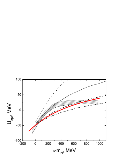
Figure 1: Energy dependence of the nucleon optical potential for $N=Z,V=0$. Results for different values of the nucleon effective mass (8) $m^{\star}_{N}/m_{N}=$0.54, 0.71, 0.8 and 0.85 calculated in the Walecka model [47] are plotted by dotted, thin continuous, dashed and dashed-dotted lines, respectively. The solid line corresponds to our calculations with parameter choice (51). Shaded area shows uncertainties in extrapolation from finite nuclei to cold nuclear matter [47].

The ratios $x_{mb}$ (see Eq. (31)) are not well fixed experimentally. Different possible choices are reviewed in [51, 52]. Within a quark counting model (cf. ”case I” of Ref. [18]) one gets $x_{mb}=1$ for non-strange baryons (in our case $\Delta$’s) and

$$x_{\omega\Lambda}=x_{\omega\Sigma}=x_{\omega\Sigma^{*}}=x_{\rho\Sigma}=x_{\rho\Sigma^{*}}=x_{\rho\Lambda}=2x_{\omega\Xi}=2x_{\rho\Xi}=\frac{2}{3}$$ (57)

in the strange sector, whereas the constituent $SU(6)$ quark model, gives different values, e.g., $x_{\rho\Xi}=1$, $x_{\rho\Lambda}=0$. In this paper we use the quark counting values first and then allow for a variation of these parameters.

The ratios $x_{\sigma h}$ are determined with the help of the relations (compare with [18]):

$$E^{h}_{\rm bind}(n_{0})=(g_{\omega N}^{2}n_{0}/[\eta_{\omega}(n_{0})\ m_{\omega}^{2}])x_{\omega h}-(m_{N}-m_{N}^{*}(n_{0}))\ x_{\sigma h},$$ (58)

where $E^{h}_{\rm bind}(n_{0})$ is the binding energy for the hyperon $h$. There is a convincing evidence from the systematic study of hypernuclei that for $\Lambda$ particles $E_{\rm bind}^{\Lambda}\simeq-30$ MeV. For $\Xi$ we adopt the value $E_{\rm bind}^{\Xi}\simeq-18$ MeV and for $\Sigma$ hyperon $E_{\rm bind}^{\Sigma}\simeq-10$ MeV (following ”case I” of [18]) is taken. There are no experimental data for $\Sigma^{*}$. For $\Sigma^{*}$ we take the same value as for $\Sigma$. One could use other parameter choices within experimental error bars, e.g. following ”cases II-IV” of Ref. [18].

We put the coupling $g_{\omega\pi}=0$, because $\omega$ does not decay in two pions. As follows from the $\pi^{-}$ atomic data, one needs a slight $\pi^{-}$ energy shift upward, $\sim 10\div 30$ MeV for $N=Z$ at the saturation density $n_{B}=n_{0}$, cf. [53]. The value of the pion $\Sigma$-term estimated from scattering data is rather small: $\Sigma_{\pi N}\simeq 30\div 45$ MeV. Since both these values (energy shift and $\Sigma_{\pi N}$) are small, we can assume $g_{\omega\pi}=g_{\sigma\pi}\simeq 0$. The $p$-wave $\pi NN$ and $\pi N\Delta$ interactions are disregarded within our RMF-based model, as all other $p$-wave effects. Thus for $N=Z$ we deal with free pions.

The $\rho\pi$-meson coupling $g_{\rho\pi}$, which is necessary to describe the pion behavior in isotopically asymmetric matter, can be found by matching with the $s$-wave Weinberg-Tomazawa term of $\pi^{-}$ polarization operator

$$g_{\rho\pi}R_{0}\rightarrow n_{n}/(2f_{\pi}^{2})\quad\mbox{for}\quad n_{B}\rightarrow 0,\ Z=0,$$ (59)

as it is motivated by the chiral symmetry, $f_{\pi}=93$ MeV, cf. [22]. Thus one gets

$$g_{\rho\pi}\simeq\frac{m_{\rho}}{2g_{\rho N}\ f_{\pi}^{2}}~{}.$$ (60)

The corresponding value $g_{\rho\pi}\simeq 6$ is consistent with that follows from the universality relation, cf. [25].

For the kaon coupling constants, we take $g_{\omega K}=g_{\omega N}/3$, $g_{\rho K}=\frac{1}{2}g_{\rho N}$ as follows from quark counting, cf. [51], and $g_{\sigma K}$ is evaluated from the $K^{+}$ and $K^{-}$ optical potentials at $n_{B}=n_{0}$ :

$$U_{\rm opt}^{(K^{+}/K^{-})}(n_{0},T=0)=-g_{\sigma K}\ \sigma(n_{0},T=0)\pm g_{\omega K}\ \omega_{0}(n_{0},T=0)~{}.$$

The experimental values of $U_{\rm opt}^{K^{+}}(n_{0},T=0)$ are in the range $\simeq 20\div 30$ MeV. It is known that the $\Sigma_{KN}$ sigma term is significantly larger than $\Sigma_{\pi N}$. However the former quantity is not well determined and may vary in a broad range, $\Sigma_{KN}\sim 150\div 400~{}$MeV. The values of a deep potential $U_{\rm opt}^{K^{-}}(n_{0},T=0)\simeq-100\div-200$ MeV are derived in Refs. [54] from analysis of kaonic atom phenomenology, whereas self-consistent calculations based on a chiral Lagrangian [20] and coupled-channel $G$ matrix theory within meson exchange potentials [55] yield $U_{\rm opt}^{K^{-}}(n_{0},T=0)\simeq-50\div-80$ MeV. In Ref. [18] the effective value $\Sigma_{KN}\simeq 150$ MeV is extracted using the analysis of the kaon-nucleon scattering of [20]. Thereby, we apply a shallow $K^{-}$ potential $U_{\rm opt}^{K^{-}}(n_{0},T=0)\simeq-80$ MeV. For the $K^{+}$ potential we take $U_{\rm opt}^{K^{+}}(n_{0},T=0)=21.4$ MeV. With these potentials we find coupling constants

$$(A):\mbox{\hskip 28.45274pt}g_{\sigma K}^{*}=0.13\ g_{\sigma N},\mbox{\hskip 28.45274pt}g_{\omega K}^{*}=\frac{1}{3}g_{\omega N}.$$ (61)

The density dependence of the $U_{\rm opt}^{K^{-}}$ and $U_{\rm opt}^{K^{+}}$ is even less constrained. Thus we also use an another set of kaon couplings obtained with the help of the scaling

$$(B):\mbox{\hskip 14.22636pt}g_{\sigma K}^{*}=0.13\ g_{\sigma N}\ \chi_{\sigma}/\chi_{\sigma}(n_{0}),\mbox{\hskip 28.45274pt}g_{\omega K}^{*}=\frac{1}{3}g_{\omega N}\ \chi_{\omega}/\chi_{\omega}(n_{0})$$ (62)

in accordance with the above scaling hypothesis.

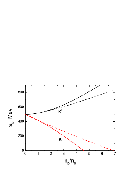
Figure 2: Kaon and antikaon energies for ${\vec{p}}=0$ as a function of the baryon density for $N=Z$, $T=0$, $V=0$ for two sets of couplings: Solid curves are for the $(A)$ set without scaling, Eq. (61), and dashed curves are for the $(B)$ set with scaling, Eq. (62).

In Fig. 2 the kaon and antikaon dispersion curves are shown versus the baryon density for iso-symmetric system at vanishing temperature for both sets of couplings. The difference between the kaon (and antikaon) dispersion curves for these two parameter choices is tiny up to $2n_{0}$ and becomes significant at higher baryon densities. Energies of antikaons $\omega_{K^{-}}$ reach zero at $n_{B}\simeq 4.5n_{0}$ and $\simeq 7n_{0}$ for parameter sets $(A)$ and $(B)$, respectively. If a deeper $K^{-}$ optical potential is used, as suggested in [54], one obtains that $\omega_{K^{-}}=0$ at smaller density. We note that the points $\omega_{K^{-}}=0$ are not the critical points of a antikaon condensation. In HIC strangeness is conserved. Then $K^{-}$ mesons can be created only in pairs with $K^{+}$ mesons at $T=0$, if the hyperon Fermi seas are not filled. Then the condensation condition for kaons and antikaons looks like $\omega_{K^{\pm}}(p=0)\pm\mu_{\rm str}=0$. In the case of infinitely long-living matter the strangeness is not conserved, and we would deal with the kaon condensation at $\omega_{K^{-}}=0$ for $T=0$. The consideration of the dense $N=Z$ system at $T=0$ has only pedagogical interest, however.

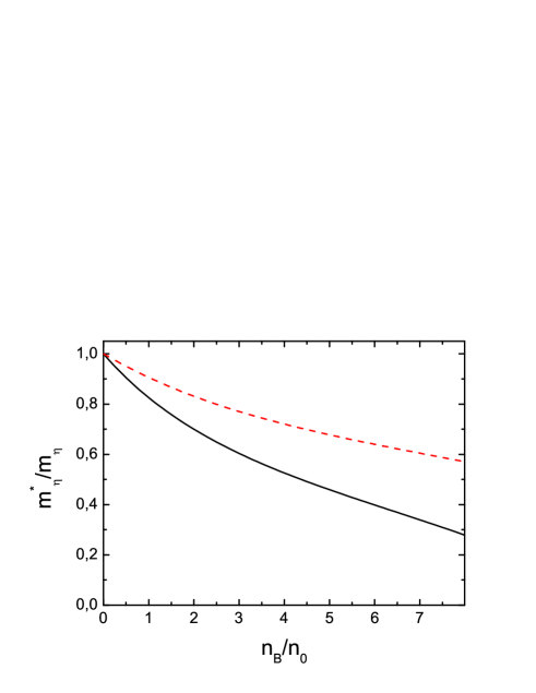
Figure 3: Effective $\eta$ meson mass given by Eq. (81) in Appendix A as a function of the baryon density for $N=Z$, $T=0$, for two sets of couplings. Solid curve: $\Sigma_{\eta N}=280~{}$MeV, $\kappa_{\eta N}=0.4~{}$fm. Dash curve: $\Sigma_{\eta N}=140~{}$MeV, $\kappa_{\eta N}=0.2~{}$fm.

Effect of the $\eta$-meson on thermodynamic quantities is minor. In our calculations of characteristics of HIC we take $\Sigma_{\eta N}\simeq 140$ MeV, $\kappa_{\eta N}=0.2$ fm (see Eq. (19)). These values are twice smaller than the average-weighted values $\Sigma_{\eta N}\simeq 280$ MeV, $\kappa_{\eta N}=0.4$ fm used in Ref. [30]. We make this choice in order to simplify the consideration by avoiding a possibility of $\eta$ condensation in a wide baryon density - temperature range of our interest. Differences of these two parametrization in the $\eta$ meson mass are shown in Fig. 3.

In case when there is no information on interactions of a particle with mean $\sigma$-, $\omega$- and $\rho$-meson fields, or if it is known that this interaction is rather weak, we treat this particle as a free one. As we have mentioned, we consider $\eta^{\prime}(958)$, $K^{*}(892)$ and $\varphi(1020)$ as free particles. We also consider $\Omega$ and $\Xi^{*}$ as free ones. For $\Sigma^{*}$ we use the same couplings as for $\Sigma$.

Though the constructed model describes arbitrary iso-asymmetric systems, in this paper we further focus on the study of isospin-symmetric nuclear matter, $N=Z$, and disregard small Coulomb effects. In calculations presented below we use by default parameters (52), (57), (62), unless other is specified.

5 SHMC EoS for $T=0$ and $N=Z$

At vanishing temperature our model differs from that of KVOR [12] in two aspects: (i) we take into account a possibility of occupation of the Fermi seas by different baryon species at higher baryon densities; (ii) we incorporate a possibility of condensation of the (quasi)Goldstone boson fields, when it occurs.

The left panel of Fig. 4 shows the baryon density dependence of the ratio of the effective mass to the bare mass for nucleons and $\omega$ and $\rho$ excitations, $m_{N}^{*}/m_{N}=m_{\omega}^{\rm part*}/m_{\omega}=m_{\rho}^{\rm part*}/m_{\rho}=\Phi$ for $\Phi>0$, see Eqs. (8) - (11), and (44), as well as for $\sigma$ excitations, $m_{\sigma}^{\rm part*}/m_{\sigma}$, given by Eq. (43) for $T=0$.

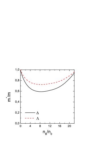
Figure 4: Baryon density dependence of the effective-to-bare mass ratio at $T=0$, $N=Z$. Left panel: for nucleon- $\omega$-$\rho$ excitations (solid line), and for $\sigma$ excitations (dashed line). Right panel: The same as in left panel but for the $\Delta(1232)$ isobar (solid line) and the $\Lambda(1116)$ hyperon (dashed line).

We observe that the effective masses monotonically decrease up to a minimal value at the density $n_{B}<n_{min,B}\simeq 8n_{0}$ and then begin to grow. This is a consequence of the fact that within our model the masses depend non-linearly on the $\sigma$ field and this dependence is determined within self-consistent calculations. Due to this feature the SHMC model EoS is getting stiffer with increasing baryon density in the range $n_{B}<n_{min,B}$ and then it becomes softer for $n_{B}>n_{min,B}$. Such a high-density behavior could additionally favor the deconfinment phase transition at large densities ($n_{B}>n_{min,B}$) at $T=0$ if it had not yet happened at a smaller density. We could chose model parameters in such a way that the value of $n_{min,B}$ would be smaller, in favor of shifting the position of the deconfinment transition to smaller density. However it would result in the simultaneous decrease of the maximum neutron star mass $<1.9~{}M_{\odot}$. The latter may come in conflict with experimental data on neutron stars, see [4].

Note that the non-linear density dependence of the nucleon and $\sigma$ effective masses resembles the density dependence of the chiral and gluon condensates obtained in Refs. [56, 57].

In the right panel of Fig. 4 we show effective masses of the $\Delta(1232)$ isobar and the $\Lambda(1116)$ hyperon, as representative examples of heavy baryon species. Their baryon density dependence is similar to that for the nucleon, with the same value of $n_{min,B}$. However the value of $m^{*}_{b}(n_{min,B})/m_{b}$ ($b\neq N$) is higher than $m^{*}_{N}(n_{min,B})/m_{N}$.

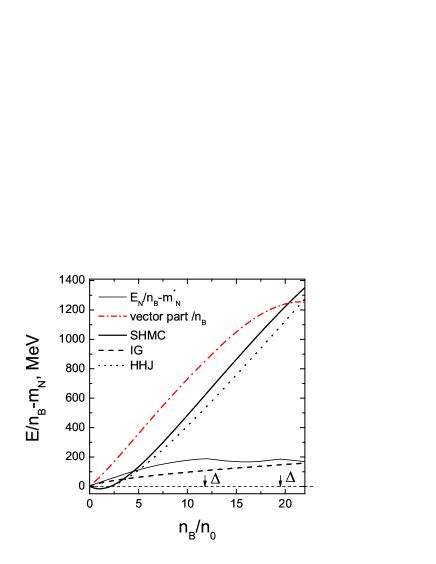
Figure 5: Baryon density dependence of the total energy per baryon (solid line) for SHMC EoS, for A18+$\delta v$+UIX* in the HHJ parametrization [41] (dotted line), and for the IG EoS (dashed line); $T=0$, $N=Z$. Arrows show the threshold densities for the appearance and melting of the $\Delta$ isobar Fermi sea. Dashed-dotted curve is a partial contribution of the repulsive vector field term of the SHMC EoS. For comparison the kinetic energy $E_{N}/n_{B}-m^{\star}_{N}$ for the SHMC model is shown by the thin continuous line.

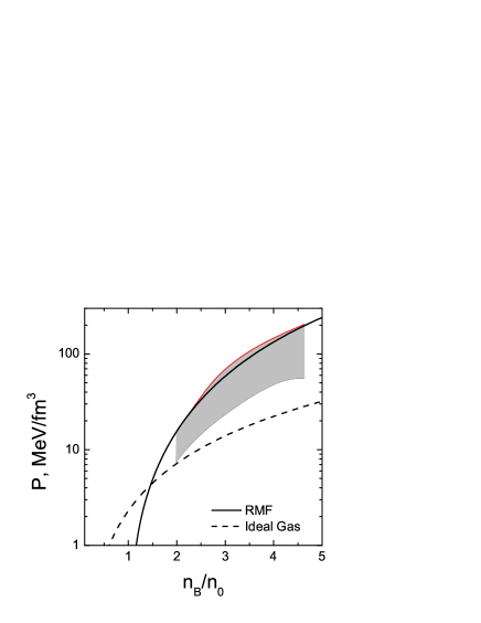
Figure 6: Baryon density dependence of pressure for symmetric nuclear matter at $T=0$ for the SHMC (solid line) and IG (dashed) EoS. The shaded area corresponds to the experimental constraint derived from HIC [59].

In Fig. 5 we show the density-dependent total energy per baryon for SHMC EoS in comparison with that for the Urbana-Argone (A18+$\delta v$+UIX*) EoS [39] (in the HHJ version of Ref. [41]) and for the ideal gas (IG) EoS. Within the IG model we include the same particle species, as in the SHMC model, but in this case all mean fields and thus all particle interactions are switched off. Thus, in the IG model at $T=0$ only nucleon Fermi seas contribute. It is seen that difference between SHMC EoS and IG EoS grows strongly with the density increase indicating to an important contribution of particle interactions. The threshold density for the appearance of the $\Delta(1232)$ isobars is $\sim 12~{}n_{0}$ and their Fermi sea again melts for $n_{B}>20~{}n_{0}$ (these densities are shown by arrows in Fig. 5). Appearance of $\Delta$’s almost does not affect the total energy per baryon. Hyperons do not occur at all for $N=Z$ in contrast with $\beta$-equilibrium matter, cf. [18].

Though baryon and meson masses begin to increase for $n_{B}>n_{min,B}$, this only moderately affects the stiffness of the EoS, since the suppression of the nucleon kinetic term (thin solid line in Fig. 5) is largely compensated by the increase of the repulsive vector meson term (dashed-dotted line in Fig. 5). Due to that SHMC EoS remains stiffer for $n>n_{min,B}$ compared to the HHJ EoS (dotted line in Fig. 5).

The SHMC EoS begins to differ from the HHJ EoS for $n_{B}>4n_{0}$ and this difference increases with increase of the baryon density. Such a behavior, cf. [12], results in an increase of the value of the maximum neutron star mass, $M_{max}=2M_{\odot}$, that is in agreement with the value $M_{max}=(2.1\pm 0.2)M_{\odot}$ (at the $1\sigma$ confidence level) derived in [58] from the observations of the PSR J0751+1807, a millisecond pulsar in a binary system with a helium white dwarf secondary.

In Fig. 6 the pressure calculated in the SHMC model (solid line) is compared with the experimental constraints coming from the analysis of elliptic flow in HIC [59]. As it has been argued in [4], only the EoS with pressure curves, being close to the upper boundary of the band, satisfies the maximum neutron star mass constraint. Pressure within the IG model of EoS (dashed line) does not fulfill the HIC flow constraint. To satisfy the flow constraint at $T=0$, one definitely needs a much stiffer EoS than that given by the IG model.

Transport calculations [60] have demonstrated that subthreshold $K^{+}$ production may provide an important information to constrain the EoS of the warm symmetric nuclear matter for $n_{B}\stackrel{{\scriptstyle\scriptstyle<}}{{\phantom{}{}_{\sim}}}3~{}n_{0}$. Within the last decade the KAOS collaboration at GSI performed measurements of the kaon production [61]. Analysis of the data [62] led to a conclusion that the EoS satisfying the kaon data is compatible with the above-required flow constraint. Both constraints hold true with the EoS of the Urbana-Argonne group (${\rm{A18}}+\delta v+{\rm{UIX}}^{*}$) and with the KVOR-based SHMC EoS used here.

6 SHMC EoS for $T\neq 0$ and $N=Z$

6.1 Density-temperature dependence of effective masses of excitations

The effective masses of the nucleon and $\omega$/$\rho$ excitations follow the same scaling law and coincide, see Eqs. (11), (43), (44). As it is seen from the left panel of Fig.7, at the baryon density $n_{B}<6\div 8~{}n_{0}$ and $T\stackrel{{\scriptstyle\scriptstyle<}}{{\phantom{}{}_{\sim}}}190$ MeV, the effective masses of the nucleon and $\omega$/$\rho$ excitations and the $\sigma$ excitation decrease when the density grows up and then they start to increase at higher densities similarly to the case $T=0$.

Generally, different phase states can be realized within the SHMC model. At some density $n_{B}=n_{B}^{\sigma\pi}$ and temperature $T=T^{\sigma\pi}$ the $\sigma$ excitation mass may reach the value $2m_{\pi}$. Then the decay $\sigma\rightarrow 2\pi$ becomes forbidden at higher $T$ and $\mu_{B}$. Ref. [63] argued that due to long-scale field fluctuations the scattering length of two pions at rest should go to infinity at $n_{B}\rightarrow n_{B}^{\sigma\pi}$, identically to the so called ”Feshbach resonance” at zero energy to be used in atomic physics for cold trapped atoms. The result is also known as a new ”strong coupling” regime of matter which manifests a liquid-like behavior [64]. However these interesting questions are beyond the scope of the present paper since in the SHMC model the particle excitations have no widths. Therefore we continue to apply our model without any modifications also for $n_{B}>n_{B}^{\sigma\pi}$.

In addition, the $\sigma$ excitation mass reaches the value $m_{\pi}$ at some density $n_{B}^{\rm chir}$ and temperature $T=T^{\rm chir}$. Note that in models with inherent chiral symmetry the $\sigma$ and $\pi$ masses meet at the chiral symmetry restoration point. As it is seen from Fig. 7, with the SHMC model for the $T=0$ case the $\sigma$ excitation mass remains always higher than the double pion mass. But at sufficiently high temperature, $T\stackrel{{\scriptstyle\scriptstyle>}}{{\phantom{}{}_{\sim}}}190~{}$ MeV, both points, $n_{B}=n_{B}^{\sigma\pi}$ and $n_{B}^{\rm chir}$, are reached.

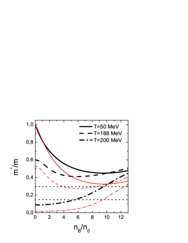
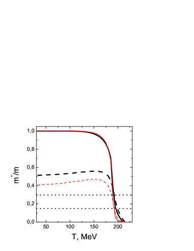
Figure 7: The effective masses of the nucleon, $\omega$, $\rho$ excitations (thick lines), and of $\sigma$ meson excitations (thin lines), $N=Z$. Two dotted straight lines show the $\sigma$ mass levels $m_{\sigma}=2m_{\pi}$ and $m_{\sigma}=m_{\pi}$ (bottom). Left panel: The baryon density dependence at different temperatures. Right panel: Temperature dependence at the baryon density $n_{B}=0$ (continuous lines) and $n_{B}=5n_{0}$ (dashed lines).

As follows from the left panel of Fig. 7, for the phase range $T\stackrel{{\scriptstyle\scriptstyle<}}{{\phantom{}{}_{\sim}}}190~{}$MeV and $n_{B}<(6\div 8)~{}n_{0}$ the density behavior of effective masses is similar to that in models with inherent partial restoration of the chiral symmetry. The values of effective masses decrease at low densities with the temperature increase in accordance with behavior of $\Phi=1-f$. For $T>190$ MeV all the effective masses are getting small rather sharply but then grow slowly with the increasing density. At temperature $T=$188 MeV the critical value $n_{B}^{\sigma\pi}$ is reached first at $n_{B}^{\sigma\pi}\approx 4n_{0}$ and this phase state is left at $n_{B}^{\sigma\pi}\approx 8n_{B}$ (see crossing of the thin dashed line with the horizontal one). At $T=200~{}$MeV the mass of the $\sigma$ field is less than $m_{\pi}$ for $0\leq n_{B}\stackrel{{\scriptstyle\scriptstyle<}}{{\phantom{}{}_{\sim}}}10n_{0}$.

As it is seen from the right panel of Fig. 7, the temperature dependence of the effective masses of nucleon and sigma excitations is small up to $T\sim 170\div 180$ MeV. For higher temperatures the effective masses begin to decrease abruptly and for $n_{B}=0$ we have $T^{\sigma\pi}\approx T^{\rm chir}\approx 190~{}$MeV. If one proceeds to the dense matter ($n_{B}=5n_{0}$) the difference between these temperatures is about few MeV. Within this narrow temperature interval the second derivative of the effective mass with respect to temperature changes the sign. The effective nucleon-$\omega$-$\rho$ and $\sigma$ excitation masses reach zero at the same critical temperature $T_{c\sigma}$, about 210 MeV. Since the coupling scaling functions $\chi_{\sigma}$ and $\chi_{\omega}$ follow the same dropping trend as the mass scaling function $\Phi$, in vicinity of $T_{c\sigma}$ we deal with a gas of almost massless excitations. Similar result has been obtained in [65] using a generalized local symmetry approach and vector manifestation arguments. The anti-nucleon yield rapidly increases due to a sharp decrease of the nucleon mass.

For $T>T_{c\sigma}$ the effective nucleon mass becomes negative. For the first time such a behavior of the nucleon effective mass has been found within the standard RMF model including $\Delta$ resonance in [66]. Authors suggested a specific choice for the resonance-$\sigma$ couplings that allows to restore positiveness of masses. Actually in the region where the effective nucleon mass is negative nothing dramatic happens. The nucleon spectrum given by Eqs. (27), (28) continues to be well defined since these equations enters $m_{N}^{*2}$ rather than $m_{N}^{*}$.

Note that in our model the effective $\omega$ and $\rho$ excitation masses follow the law (11), (44). Thus they only touch zero at $T=T_{c\sigma}$ and become again positive for $T>T_{c\sigma}$. Therefore $\omega$ and $\rho$ condensates should not appear at $T>T_{c\sigma}$.

However the effective mass of the $\sigma$ excitation ($m_{\sigma}^{\rm part*}$, see Eq. (66 ) in Appendix A) is getting imaginary at $T>T_{c\sigma}$. Thus, the ground state proves to be unstable with respect to the Bose condensation of the $\sigma$ excitation field. The stability is achieved due to the self-interaction between the $\sigma$-particle excitations, see Appendix B. Such a condensation might be called ”hot Bose condensation” since it occurs at $T>T_{c\sigma}$, in contrast with the standard Bose-Einstein condensation appearing with the temperature decrease. A possibility of hot Bose condensation has been considered in [24], within a different model which includes effects of particle widths. In order not to complicate consideration we avoid description of temperature region above $T_{c\sigma}$ in the present work.

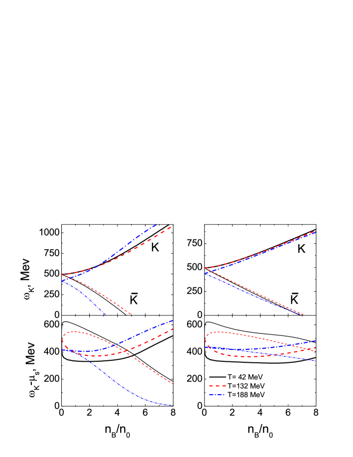
Figure 8: Baryon density dependence of energies $\omega_{K}$ (upper panels)) and $\omega_{K}-\mu_{s}$ (lower panels) for kaons (thick lines) and antikaons (thin lines) at ${\vec{p}}=0$ at three values of the temperature $T=$42, 132 and 188 MeV, $N=Z$. Left panel: the $(A)$ set for kaon couplings without scaling, Eq. (61). Right panel: for the $(B)$ set of couplings with scaling, Eq. (62).

Fig. 8 (upper panels) presents the baryon density dependence of the energy for kaons ($K^{+}$ or $K^{0}$) and antikaons ($K^{-}$ or $\bar{K}^{0}$) with zero momenta at three values of temperature, see Eqs. (77)-(79) of Appendix A. Kaons ($K^{+}$ and ${K}^{0}$) (as well as antikaons ($K^{-}$ and $\bar{K}^{0}$)) have the same dispersion relations in the iso-symmetrical matter, if a small Coulomb contribution is neglected. We see that the $K^{+}$ energy only slightly depends on the temperature for $T\stackrel{{\scriptstyle\scriptstyle<}}{{\phantom{}{}_{\sim}}}170~{}$MeV, $\omega_{K^{+}}$ decreases with the $T$ increase. Temperature dependence of the $K^{-}$ energy is also minor for $T\stackrel{{\scriptstyle\scriptstyle<}}{{\phantom{}{}_{\sim}}}170~{}$MeV, $\omega_{K^{-}}$ increases with the $T$ increase. Thus for $T\stackrel{{\scriptstyle\scriptstyle<}}{{\phantom{}{}_{\sim}}}170~{}$MeV the density dependence remains similar to that at $T=0$, see Fig. 2. For higher temperatures the $T$ dependence becomes significant for both kaons and antikaons. At $n_{B}=0$, branches $\omega_{K^{+}}$ and $\omega_{K^{-}}$ coincide. For set $B$ of scaled couplings the dispersion curves are more flat than for set $A$. For set $A$, $\omega_{K^{-}}$ vanishes at $n_{B}\sim(3\div 5)n_{0}$ (for $T\leq 188~{}$MeV) and for set $B$, for $n_{B}\sim 7n_{0}$. However it does not mean that the condensation occurs. The necessary condition for condensation is $\omega_{K}({\vec{p}}=0)-\mu_{s}=0$, $\mu_{s}=\mu_{\rm str}$ for kaons and $\mu_{s}=-\mu_{\rm str}$ for antikaons, see Eq. (83) of Appendix A. This difference is plotted in the bottom part of Fig. 8. It is seen that the kaon condensation condition is never fulfilled. Antikaon condensation takes place only if the density-dependent scaling is neglected (set $A$), at $n_{B}\sim 8n_{0}$ and $T\sim 190~{}$MeV. With set $B$ of couplings the antikaon condensation does not occur in the relevant density-temperature range. Therefore we perform subsequent calculations of HIC for the case $B$.

Figure 9: Baryon density dependence of the $\eta$ effective mass at four values of the temperature $T=$42, 132, 188 and 200 MeV, $N=Z$, for $\Sigma_{\eta N}=140$ MeV and $\kappa_{\eta N}=0.2$ fm.

Fig. 9 shows that the $\eta$ effective mass monotonically falls down with the baryon density if the temperature is not very high. However at $T\sim 200~{}$MeV the $\eta$ effective mass becomes almost independent of $n_{B}$ for $n_{B}\stackrel{{\scriptstyle\scriptstyle<}}{{\phantom{}{}_{\sim}}}12n_{0}$, $m_{\eta}^{*}/m_{\eta}\simeq 0.4$, within the $n_{B}-T$ region depicted in Fig. 9. For $n_{B}\stackrel{{\scriptstyle\scriptstyle>}}{{\phantom{}{}_{\sim}}}15n_{0}$ the in-medium $\eta$ mass practically is independent of temperature. The $\eta$ condensation does not appear for $T\leq T_{c\sigma}$. If we used parameter choice $\Sigma_{\eta N}=280$ MeV and $\kappa_{\eta N}=0.4$ fm (see solid line in Fig. 3) we would meet with the $\eta$ condensation problem.

6.2 SHMC EoS for baryonless matter.

Now let us consider the case $n_{B}\simeq 0$ that is close to conditions realized at RHIC. The decrease of the hadron masses with increase of the temperature for $n_{B}\simeq 0$ has been found in [24] as the consequence of the blurring of the baryon and meson vacuum. Here we obtain a similar effect but within the quasiparticle picture.

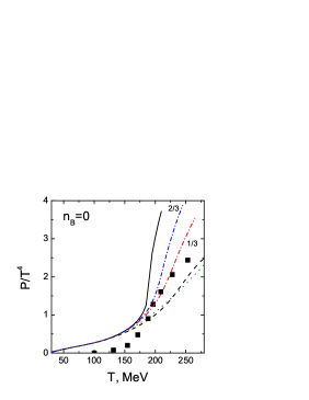
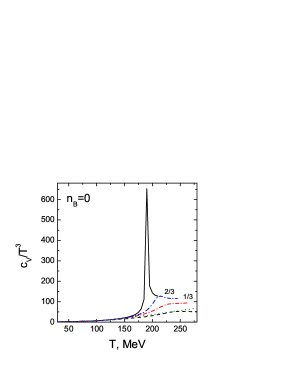
Figure 10: Temperature dependence of the reduced pressure (left) and reduced specific heat (right) for iso-symmetric baryonless matter. The solid line presents our full calculation. The dashed line shows the case when contribution of all baryons besides neutrons and protons is artificially suppressed. Two dashed-dotted lines are the case when all $g_{mb}$ couplings except for nucleons are suppressed by factors of $2/3$ and $1/3$, respectively. Squares show the lattice QCD result for the 2+1 flavor case [67]. The dotted curve is for the IG model.

In Fig. 10 temperature dependence of the pressure is shown in $T^{4}$ units (left) and the specific heat, in $T^{3}$ units (right) for $n_{B}=0$. On the left panel the solid curve presents our calculation with parameters determined in sect. 4. The dashed curve shows pressure in the case when contribution of all baryons, except neutrons and protons, is artificially suppressed while the dotted curve is given for the IG model. All curves are close to each other for $T\stackrel{{\scriptstyle\scriptstyle<}}{{\phantom{}{}_{\sim}}}160\div 170$ MeV. Differences start at higher temperatures where high-lying baryon resonances come into play. At $T=T_{c\sigma}$ the effective mass squared for the $\sigma$ excitation drops to zero and becomes negative for $T>T_{c\sigma}$. In order not to complicate the consideration we avoid discussion of the hot Bose condensation of $\sigma$ excitations. Therefore we cut the solid line at $T>T_{c\sigma}$. In the case when baryon resonance contributions (except nucleons) are artificially suppressed, the effective nucleon mass as well as the $\sigma$ excitation mass approach zero only at $T\rightarrow\infty$ (if $\eta$ is a free particle, otherwise $\eta$ may condense at $T_{c\eta}\simeq 265$ MeV).

We also compare our result with the lattice QCD calculations for $2+1$ flavor [67]. One usually believes the lattice data for the quark-gluon sector (i.e. for $T>T_{\rm dec}\approx 175$ MeV and for $n_{B}\simeq 0$). On the other hand, there are doubts that the lattice calculations produce appropriate results for the hadronic sector, $T<T_{\rm dec}$, since they get unrealistically high value for the pion mass, $m_{\pi}\sim 700$ MeV, instead of the physical value $140$ MeV, cf. [67]. Recently a higher deconfinement temperature was obtained in lattice QCD calculations for similar system with almost physical value of the pion mass, $T_{\rm dec}=192(7)(4)$ [68]. However thermodynamical characteristics still have not been recalculated. Therefore we may use any hadron EoS for $T<T_{\rm dec}$ (with a not precisely known value of $T_{\rm dec}$) without referring to the lattice data. For a larger temperature, one could expect that the quark phase becomes energetically preferable. It happens if the pressure in the hadron phase is less than in the quark phase. Oppositely, Fig. 10 shows that the pressure extracted from the lattice calculations is significantly smaller than that obtained within the SHMC model for the hadron phase at $T\stackrel{{\scriptstyle\scriptstyle>}}{{\phantom{}{}_{\sim}}}170$ MeV. This may mean that we have no deconfinement phase transition with our EoS with the values of the coupling constants used. Instead, within our model we obtain a state of a high-temperature hadron gas of many baryon resonances (quasiparticles in the given model) and bosons, with small effective masses. This phase is enriched by antiparticles. As we have mentioned above, this result coincides with that of Ref. [24], though here it is obtained within a phenomenological quasiparticle scheme while in [24] it is a consequence of blurring of the hadron vacuum.

The deconfinement transition could be constructed if the (lattice) quark-gluon EoS is matched with our EoS for lower $T$ ($T_{\rm dec}\stackrel{{\scriptstyle\scriptstyle<}}{{\phantom{}{}_{\sim}}}160$ MeV) when our hadron phase pressure is not yet too high (compare solid and dashed lines in Fig. 10). Another possibility for the deconfinment transition can be associated with a different mechanism: The overlapping of the hadron cores, if hadrons are considered as composite particles. We have a dramatic increase of hadron degrees of freedom at $T\stackrel{{\scriptstyle\scriptstyle>}}{{\phantom{}{}_{\sim}}}170$ MeV. Thus the hadron cores may become overlapping for such temperatures. If this mechanism works, the deconfinment transition should be treated as an enforced Mott-like transition occurring due to the melting of composite hadrons, rather than matching the pressures of two different phases.

In Fig. 10 solid lines present results of calculations with the default parameters defined in sect. 4. Here we have $T_{c\sigma}\simeq 210~{}$MeV. Dashed-dotted lines demonstrate the cases when $g_{mb}$ couplings, except for nucleons, are suppressed by factors $2/3$ and $1/3$ (as indicated on the plot). The latter case (with $1/3$ prefactor) allows to fit the lattice data up to $T\sim 240~{}$MeV. In this case a quark liquid would masquerade as a hadron one. In principle one could fit the lattice data in a still larger region of temperatures (e.g., up to $500~{}$MeV) introducing $\chi_{\sigma}<\Phi$. A violation of the universality of the $\sigma$ scaling would be in a line with that we have used for $\omega$ and $\rho$, $\eta_{\omega}\neq 1$ and $\eta_{\rho}\neq 1$. However we will not elaborate this possibility in the present work. The dashed-dotted curve labelled by $1/3$ is cut at $T_{c\eta}\simeq 265~{}$MeV. At this point the $\eta$-meson mass becomes imaginary within our parametrization and $\eta$ condensate arises. If $\eta$ were treated as a free hadron, we would obtain $T_{c\sigma}\simeq 330~{}$MeV in this case.

The right panel of Fig. 10 demonstrates the temperature behavior of the specific heat for $n_{B}=0$. With the standard choice of couplings (solid curve) we observe a sharp peak with maximum at $T\simeq 190~{}$MeV. At this point the second derivative of the effective nucleon-$\omega$-$\rho$ and $\sigma$-excitation masses changes the sign. The specific heat retains a continues function. The obtained behavior is typical for the strong crossover transition. Note that such a behavior of the specific heat was also found within the standard RMF model [69]. In the case of the second-order phase transition, the specific heat would be discontinues at the critical point. When $g_{mb}$ couplings are suppressed, the peak is smoothed that reminds about a weak crossover. Often the temperature at the maximum of the specific heat is associated with the critical temperature of a phase transition. However note that in our case the position of this maximum $T\simeq 190~{}$MeV slightly differs from the $T=T^{\rm chir}$ and it differs also from $T_{c\sigma}$ ($\sim 210~{}$MeV), see Fig. 7. This fact of non-unique value of the critical temperature $T_{c}$ is also manifested in the lattice calculations: Analysis of different thermodynamic quantities leads to different numerical values of $T_{c}$ even in the continuum and thermodynamic limits [70]. One should keep in mind that there is no liberation of internal (quark-gluon) degrees of freedom of hadrons in the RMF models. Note that the $P/T^{4}$ curve calculated in the IG model is below our result even if only nucleons are taken into account (compare dotted and dashed curves in left panel of Fig. 10). This is due to the decrease of the nucleon mass with increasing temperature in the SHMC model. The specific heat $c_{V}/T^{3}$ in the IG model does not saturate for high $T$, whereas all curves of the SHMC model tend to constant values.

6.3 SHMC EoS for $n_{B}\neq 0$

In Fig. 11 we show temperature dependence of the pressure (left) and specific heat (right) for baryon densities $n_{B}/n_{0}=$2, 5 and 10.

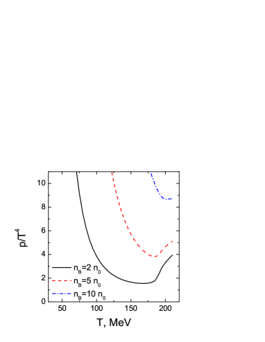
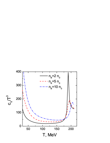
Figure 11: Temperature dependence of the pressure (left) and specific heat (right) at $n_{B}\neq 0$ for $N=Z$ for three values of $n_{B}$.

The pressure gets minimum at temperature $T\simeq(175\div 200)~{}$MeV and grows for higher $T$. The calculations are stopped at $T=T_{c\sigma}$ as was mentioned above. The value $T_{c\sigma}$ depends on $n_{B}$ only moderately. We see that the peak of the specific heat survives at finite baryon density. The value of the temperature $T_{\rm max}$ corresponding to the peak is slightly shifted up with the baryon density but the hight of the peak changes significantly. In particular, the position of the $c_{v}/T^{3}$ maximum is $T_{\rm max}\sim 190~{}$MeV at $n_{B}\stackrel{{\scriptstyle\scriptstyle<}}{{\phantom{}{}_{\sim}}}2n_{0}$ and moves to about 200 MeV for the density $n_{B}=10n_{0}$.

6.4 Particle densities

The particle density of species $i$ is given by

$$n_{i}=g_{i}\int\frac{d^{3}p}{(2\pi)^{3}}\ f_{i}(p)~{},$$ (63)

where the spin-degeneracy factor $g_{i}=(2s_{i}+1)$ and $f_{i}$ is the particle occupation function, see Eqs. (28)-(30),(82),(83). In the SHMC model the spectra of most particle species are getting softer with the baryon density increase because of in-medium effect. This occurs for all baryons and for $\omega$ and $\rho$ due to the scaling of the effective masses, as well as for $\sigma$ and (quasi)Goldstone excitations ($K^{-}$, $\bar{K}^{0}$ and $\eta$) as a consequence of their interaction with mean fields. Therefore the densities of these particle species are larger than in the IG case.

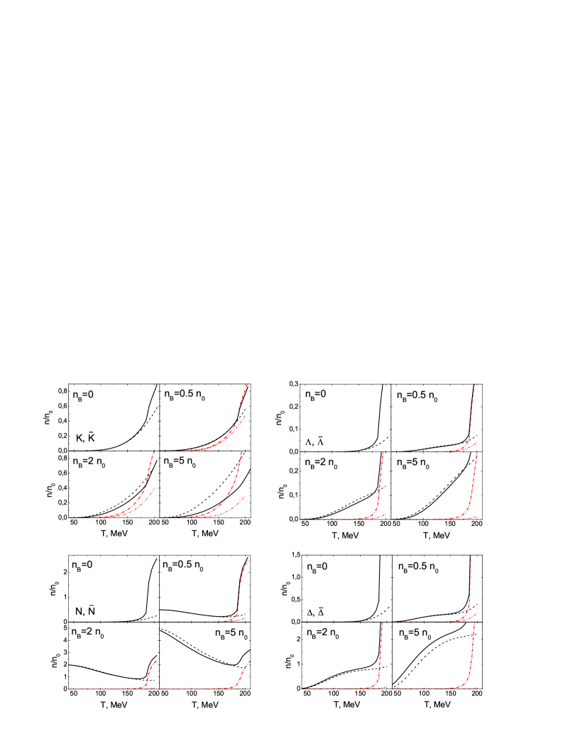
Figure 12: Particle number density in $n_{0}$ units versus temperature at different baryon densities for $K,\Lambda,N,\Delta$ and their antiparticles, $N=Z$. Our model results are plotted by solid line for particles and by dashed-dotted line for antiparticles. Dashed and dashed-double-dotted curves correspond to particles and antiparticles in the IG model.

Temperature dependence of the density for various particle species (and for their antiparticles) for iso-symmetric matter at different values of baryon densities is shown in Fig. 12. In the $n_{B}=0$ case the particle and antiparticle yields coincide. As it is seen, all the species besides nucleons exhibit very similar behavior (compare solid and dashed lines). Particle number density slowly grows with the temperature increase till $T\sim 170~{}$MeV and then rapidly goes up. In the range $T\stackrel{{\scriptstyle\scriptstyle<}}{{\phantom{}{}_{\sim}}}170~{}$MeV the SHMC results are rather close to those of the IG model (except for a high density, see example $n_{B}=5n_{0}$) but drastically diverge at higher temperatures. This difference is naturally explained by the rapid decrease of in-medium masses in the SHMC model at these temperatures (see Figs. 4,7). In contrast, at $T\stackrel{{\scriptstyle\scriptstyle<}}{{\phantom{}{}_{\sim}}}170~{}$ MeV the nucleon density $n_{N}$ stays almost independent of temperature at $n_{B}\simeq 0.5n_{0}$, or significantly decreases at higher $n_{B}$. These facts are due to a stabilization effect of the baryon conservation law and a strong growth of production of baryon excited states and hyperons with the baryon density increase (cf. $\Delta$ and $\Lambda$ particle densities in Fig. 12). Similarly to other species, the nucleon particle density rapidly goes up with further temperature increase (for $T\stackrel{{\scriptstyle\scriptstyle>}}{{\phantom{}{}_{\sim}}}170~{}$MeV).

Temperature-density behavior for antiparticles is quite different. In spite of the fact that the iso-symmetric system is considered, even for IG the densities of created kaons and antikaons are different (except for the $n_{B}=0$ case). This is a consequence of the total strangeness conservation which takes into account also hyperon species. Thus $\mu_{\rm str}$ proves to be non-zero even for $N=Z$ that results in $n_{K^{+}}\neq n_{K^{-}}$. Although the correction to the energy dispersion curve is positive (repulsion) for kaons and negative (attraction, see Fig. 2) for antikaons, their number densities intersect at temperature $160\stackrel{{\scriptstyle\scriptstyle<}}{{\phantom{}{}_{\sim}}}T\stackrel{{\scriptstyle\scriptstyle<}}{{\phantom{}{}_{\sim}}}180~{}$MeV for $n_{B}\neq 0$ and then, with the subsequent temperature increase, the antikaon density even exceeds that for kaons. But it is only apparent violation of strangeness conservation since excited kaon states $K^{*}$ contribute. Because $K^{*}$ is treated as a free particle, $n_{K^{*+}}\gg n_{K^{*-}}$ at high temperature and baryon density. In particularly, at $T=190~{}$MeV and $n_{B}=5n_{0}$ we have $n_{K}=0.46n_{0}$, $n_{\bar{K}}=0.68n_{0}$ and for the excited kaon state $n_{K^{*}}=1.15n_{0}$, $n_{\bar{K}^{*}}=0.07n_{0}$. Indeed, $n_{K}<n_{\bar{K}}$ but the total strangeness of these four kaon species is $\sim 0.8n_{0}$ which is compensated by hyperons. As for antinucleons, antideltas and antihyperons, their behavior looks very similar: the yield of all antibaryons is markedly suppressed at $T\stackrel{{\scriptstyle\scriptstyle<}}{{\phantom{}{}_{\sim}}}170~{}$MeV and abruptly grows up at higher temperature, $T\stackrel{{\scriptstyle\scriptstyle>}}{{\phantom{}{}_{\sim}}}180~{}$MeV. This increase is not reproduced by the IG model which produces significantly lower hadron densities. Generally, the baryon density dependence of the particular number density seems to be not as strong as temperature one.

7 Application of the model to HIC

The SHMC model describes the EoS of hot and dense hadronic matter in a broad range of temperatures and baryon densities. In HIC the dense matter created in the initial stage is expected to rapidly thermalize and then it expands without significant generation of the entropy $S$. In the process of expansion some particles may leave the fireball carrying away a part of the entropy. Thus more appropriate characteristic which is approximately conserved is the entropy per participant nucleon ($S/N_{B}$). This thermodynamic quantity should be conserved in quasi-equilibrium case and it is also less affected by any possible particle loss or gain from the fireball during the expansion stage. The predictions of our models for the evolution path in the $(T,\mu_{B})$-plane as obtained from the SHMC EoS under condition of the fixed $S/N_{B}$ are shown in Fig. 13.

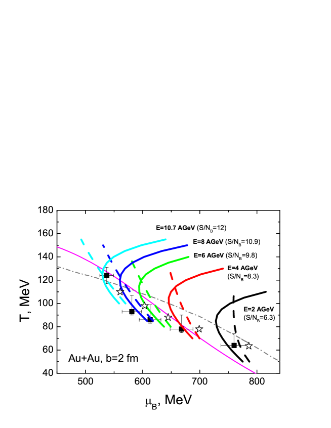
Figure 13: Isentropic trajectories for central Au+Au collisions at different bombarding energies calculated in our model (solid lines) and IG (dashed lines). Experimental points with error bars are taken from [73]. The freeze-out points marked by stars are obtained in this work (see the text below). Thin line corresponds to the freeze-out curve in [73] while dash-dotted line is that from [72].

For the initial fireball expansion stage, in the case of semi-central Au+Au collisions at different bombarding energies below the top AGS energy, the reduced entropy ratios, $S/N_{B}$, were estimated within a transport Quark-Gluon String Model (QGSM), as described in [34]. The temporal $S/N_{B}$ dependence exhibits some saturation [71], values being taken as an input for our isentropic calculations and indicated in Fig. 13. The presented isentropic curves follow exactly and unambiguously from the EoS. Some uncertainties in location of these curves are coming from uncertainties in the estimate of the reduced entropy related to the bombarding energy. In our case $\delta(S/N_{B})\sim 0.1$ and it unessentially influences the trajectory location. The $(T,\mu_{B})$ trajectories calculated within the SHMC model show turning points those positions correlate roughly with the freeze-out curve. This fact was noticed earlier in [71] where the EoS with a phase transition was used. There the high-temperature part of trajectory with $\partial T/\partial\mu_{B}>0$ was associated with the quark-gluon sector of EoS but in the present work it is due to a strong decrease of hadron masses in the considered area of the phase diagram. Note that there is no turning point in the IG case.

Two chemical freeze-out curves are shown in Fig. 13. Dashed-dotted curve corresponds to the IG EoS with the chemical freeze-out condition that the energy per hadron equals to 1 GeV ($<E>/<N>=1$ GeV) [72]. It is of interest that in the considered $(T,\mu_{B})$ range this freeze-out curve is also very close to that obtained for the IG EoS with the fixed baryon density $n_{B}=0.12\,$ fm^-3 [73]. So, the net baryon density of states above the dashed-dotted line in Fig. 13 is $n_{B}>0.8n_{0}$. Maximal densities explored in this phase diagram range from $\sim 2.3n_{0}$ to about $4n_{0}$ when the bombarding energy increases from 2 AGeV till the top AGS energy (these numbers depend on the region over which averaging was made). The thin line is obtained by interpolation of the $(T,\mu_{B})$ fitting parameters extracted at every available bombarding energy by the $\chi^{2}$ minimization of the difference between experimental and theoretical (calculated within a statistical model with the IG EoS) hadron abundance [73]. In any analysis the thermodynamic quantities $(T,\mu_{B})$ at the freeze-out are derived from the analysis of measured particle ratios. The straightforward consequence of the statistical assumption is that the mean hadron multiplicities should be calculated in the full ($4\pi$) phase space. However, due to limited experimental acceptance it is not possible to do that in each case and instead the particle ratios at the middle rapidity are used. Making use of middle rapidity ratios implies that the measured distribution $dN/dy$ is approximately constant over the same range. The analysis of the expected dispersion of rapidity distributions shows that the use of full space multiplicities is better suited over the energy ranges of AGS and SPS [75]. Unfortunately in the energy range considered in Fig. 13 the $4\pi$ particle ratio measurements are available only at two energies, and the thin line is obtained by the $(T,\mu_{B})$ interpolation based on the analysis of the middle rapidity data. Generally, both heuristic freeze-out curves describe quite well the extracted $(T,\mu_{B})$ values and they differ more noticeably in the presented range $E_{lab}\stackrel{{\scriptstyle\scriptstyle<}}{{\phantom{}{}_{\sim}}}10~{}$AGeV, below the top of AGS energy. Before to explain how freeze-out points marked by stars in Fig. 13 were obtained in the given work, we consider which hadron abundance is predicted by the SHMC model and which values of thermodynamic parameters may be inferred from comparison with experiment.

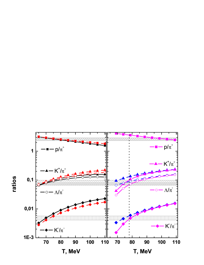
Figure 14: Particle ratios calculated along the isentropic trajectories for central Au+Au collisions at $E_{lab}=4$ AGeV. Left panel: Solid and dashed lines are calculated right before freeze-out for the SHMC and IG EoS, respectively. Right panel: Solid line is calculated in the SHMC model right after freeze-out has occurred, with taking into account the canonical strangeness suppression. Dashed line is that without strangeness suppression. Shaded bands correspond to uncertainties of experimental data [73]. The dotted vertical line is our estimate of the freeze-out temperature.

In Fig. 14 the $E_{lab}=4$ AGeV case is exemplified in detail. In the left panel the particle ratios for the most abundant hadrons are calculated along isentropic trajectories of the SHMC and IG EoS’s depicted in Fig. 13. Note that these quantities are in-medium ratios which would be ”inside” hot and dense matter right before the freeze-out, but measured ratios correspond to free particles after the freeze-out. Although trajectories are remarkably different for the IG and SHMC EoS’s, the particle ratios turn out to be not so sensitive to the choice of EoS (besides the $K^{-}/\pi^{-}$ ratio), since freeze-out baryon densities are rather low. In the right panel of Fig. 14 the particle ratios are shown just after the freeze-out.

Up to now there is no appropriate theory of the freeze-out though there exist many different recipes. Generally, transition from the collective expansion to kinetic stage and then to free particle streaming should be continuous and it takes some finite time. For the sake of simplicity some sudden approximation is often applied. If we assume a prompt freeze-out concept, the observable yield will be defined by in-medium particle spectra $dN/d^{3}p$, as we calculated them within the SHMC model, but additionally multiplied by a pre-factor $\sqrt{m^{2}+p^{2}}/\sqrt{m^{*2}+p^{2}}$ due to quasiparticle undressing, cf. [76]. However the assumption of prompt freeze-out might not be applicable at least for some particle species. Besides, one should take a especial care about the total energy conservation.

In Ref. [77] another more conventional choice was suggested. At crossing the freeze-out point (hypersurface in a general case) the change from the in-medium to IG EoS occurs in a ”shock-like” way: One demands the energy, momentum, and the net baryon charge and strangeness conservations. We do not consider the fireball expansion dynamics but use the isentropic trajectory with our EoS. Thus we know nothing about momentum conservation and in our simplified case only conservation of energy and charges is taken into account. Certainly, important collective flow effect is out of consideration. Therefore below we focus on analysis of particle ratios, where this effect is cancelled, cf. [72, 73]. We use this scenario [77] in our calculations presented in Figs. 14 (right panel) and Fig. 15. In this case the attractive in-medium interaction brings to an increase of temperature of free gas after freeze-out. As shown in the right panel of Fig. 14 (dashed lines), such a procedure results in the agreement with experiment of particle ratios at temperature by about 10 MeV higher than that inside the medium (cp. the left panel of Fig. 14). Certainly, for the IG EoS there is no changes due to the energy-momentum conservation.

All above-mentioned calculations have been done in the grand canonical ensemble. However for description of strangeness production at not too high temperatures when a number of strange particles is small, this approach is not quite appropriate and the canonical ensemble for strangeness should be used [78]. Replacement of the grand canonical description by the strangeness canonical one results in extra temperature-dependent suppression factor for strange particle densities which reaches unity for $T\stackrel{{\scriptstyle\scriptstyle>}}{{\phantom{}{}_{\sim}}}100~{}$MeV. The factor was calculated in the standard way [73, 79]. This canonical strangeness suppression effect is clearly seen from comparison of solid and dashed lines in Fig. 14 (right panel). Note that, if both effects are taken into account, the best agreement of calculated particle ratios simultaneously with all measured ones is reached at the temperature $T\simeq 78~{}$MeV which can be treated as a freeze-out temperature $T_{fr}$ in the given case (shown by the vertical line).

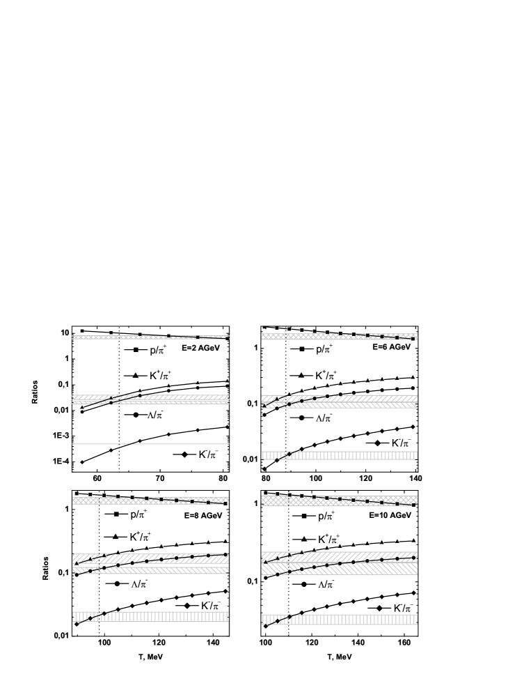
Figure 15: Particle ratios for central Au+Au collisions calculated at different collision energies. Solid lines are SMHC results at the shock-like freeze-out with taking into account canonical strangeness suppression. Shaded bands correspond to uncertainties of experimental data [73]. In the case of $E_{lab}=2~{}$AGeV the experimental line for $K^{-}/\pi^{-}$ shows only the upper limit of this ratio. The dotted vertical lines are freeze-out temperatures.

Final SHMC results for hadron ratios at other four AGS energies are presented in Fig. 15. Calculated along isentropic trajectories, these ratios take into account both the shock-like freeze-out and canonical suppression effect (compare with in-medium ratios shown in Fig. 14 for the case $E_{lab}=4$ AGeV). One can see that at every bombarding energy it is possible to fix some freeze-out temperature $T_{fr}$ by condition of the best agreement of the calculated ratios with experiment. The extracted $T_{fr}$ are shown in Figs. 14, 15 by vertical dashed lines. One should note that the proton yield includes both direct protons and those feeding from the resonance decays. However in the intermediate energy range considered, a part of protons is bound into light complex particles ($d,\alpha$). This nucleon coalescence effect is the higher, the lower the bombarding energy is, and this effect is disregarded in our model. Thus a discrepancy with experiment for $p/\pi^{+}$-ratios seen in upper panels of Fig. 15 should not be taken too seriously.

If the $T_{fr}$ on the isentropic curve is known, an appropriate baryon chemical potential for the IG EoS at the freeze-out, $\mu_{fr}$, can be found. These pairs of $(T_{fr},\mu_{fr})$ are indicated by stars in Fig. 13. The new freeze-out points, based on the same middle rapidity particle ratios, slightly differ by some shift in the chemical potential from those obtained by direct fitting of these ratios in statistical theory [73]. As to $T_{fr}$, our freeze-out temperature for $E_{lab}=10$ AGeV is noticeably below the fitted one. In contrast with lower energies, at the top AGS energy the set of 10 particle ratios was measured and used in the statistical model fit, while our results are based on 4 ratios, as shown in Fig. 15. If the $d/p,\bar{p}/p,\bar{\Lambda}/\Lambda,\varphi/K^{+}$ ratios are excluded from this analysis, then one gets $T_{fr}=108\pm 9~{}$MeV and $\mu_{B}=555\pm 18~{}$MeV [73] what is in a reasonable agreement with our result (see stars in Fig. 13). Note that this new method for deriving freeze-out points in the phase diagram allows one to keep some memory on the collision dynamics (the value of the entropy per baryon and isentropic trajectories inherent to the final expansion stage) and takes into consideration the in-medium particle modification. The freeze-out point is taken on the phase trajectory which depends on the EoS as is seen from comparison between the SHMC and IG models in Fig. 13. Note that partial ratios are sensitive to the choice of the freeze-out scenario. If we used the prompt freeze-out concept [76] we would obtain other yields.

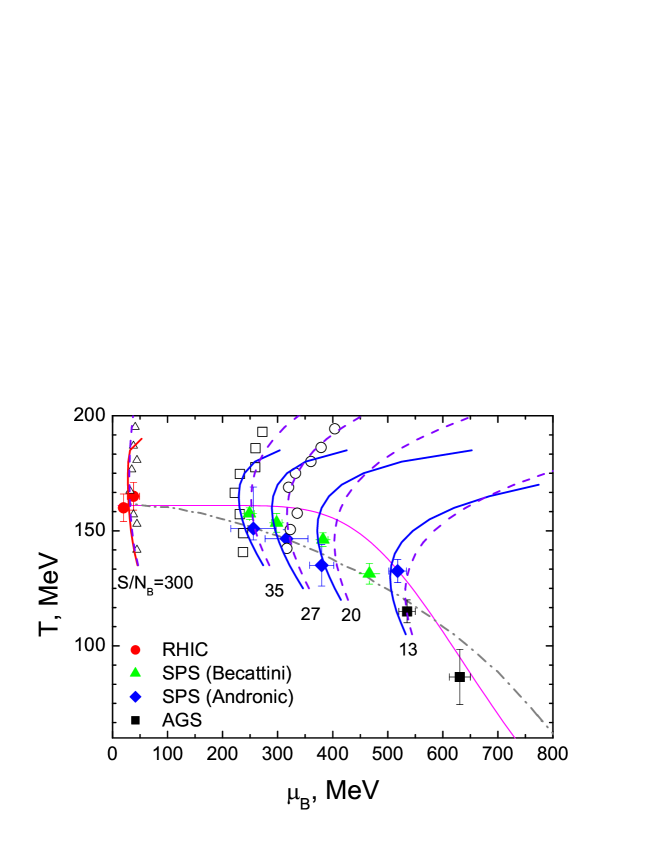
Figure 16: Isentropic trajectories for ultrarelativistic central Au+Au collisions at different bombarding energies calculated in the SHMC model with the default set of parameters (solid lines) and with the suppressed couplings by the factor 1/3 for all baryons besides nucleons (dashed lines). Filled diamonds and triangles are obtained from the $4\pi$ particle ratios in [73] and [75], respectively. Filled circles are RHIC data based on the middle rapidity particle ratios [73]. Open circles, squares and triangles are the lattice 2-flavor QCD results [81] for $S/N_{B}=$ 30, 45 and 300, respectively. Two freeze-out curves are the same as in Fig. 13.

Let us extend our analysis to higher bombarding energies. The entropy per baryon participants was calculated in [80] within the 3-fluid hydrodynamic model assuming occurrence of the first order phase transition to a quark-gluon plasma. The energy range from AGS to SPS was covered there. We use the $S/N_{B}$ values for $E_{lab}=$158, 80, 40 and 20 AGeV, at which the particle ratios were measured by the NA49 collaboration (cf. [73]). At the RHIC energy we put $S/N_{B}=300$ in accordance with the estimate in [81]. Note that in this analysis the $(T,\mu_{B})$ thermal parameters were determined using the $4\pi$ particle ratios, besides the RHIC point. The difference between two sets [73, 75] of $(T,\mu_{B})$ freeze-out points is caused by more elaborated statistical model implemented in Ref. [75]. It is of interest that both sets strongly correlate with the freeze-out curve $<E>/<N>=1$ GeV [72] and markedly differ from interpolation of the freeze-out points based on the middle rapidity particle ratios.

The calculated trajectories for isentropic expansion are presented in Fig. 16. The trajectories (solid lines) behave very similar to those at lower bombarding energies (shown in Fig. 13) exhibiting some flattening above the freeze-out curve near the expected phase boundary. Such a behavior reminds the one obtained in [82] where a smeared first-order phase transition is assumed. If baryon couplings (besides nucleons) are suppressed by a factor 1/3, the calculated trajectories turn out to be very close to the lattice QCD results [81]. Note that dealing with the finite chemical potential we use here the same choice of parameters $g_{mb}$ as in the case $n_{B}=0$ (see Fig. 10).

In principle, we could repeat our particle-ratio analysis in the SPS energy domain for both parameterizations of the SHMC model, with suppressed and not suppressed couplings $g_{mb}$. However for this aim the used SHMC model basis of hadron species should noticeably be enlarged by inclusion of higher resonances since available set of experimental data for particle ratios is significantly larger at high energies [73].

8 Conclusions and perspectives

In this paper the modified relativistic mean-field $\sigma$-$\omega$-$\rho$ model with scaled hadron masses and couplings (SHMC model) formulated for $T=0$ in Ref. [12] is generalized to finite temperatures. Besides nucleon and mean fields the model includes low-lying baryon resonances and their antiparticles, boson excitations (following the $SU(3)$ concept) and $\sigma$- $\omega$- $\rho$-excitations on the ground of mean fields. The EoS for $T=0$ satisfies general constraints known from atomic nuclei, neutron stars and those coming from the flow analysis of HIC data. Like in the KVOR model [4], we assume that $\sigma$, $\omega$, $\rho$ field mass terms, as well as nucleon masses, decrease with increase of a combination of a $\sigma$ mean field $f=g_{\sigma N}\chi(\sigma)\sigma/m_{N}$ (see Eq. (10)) corresponding to the change of the chiral condensate density. The model supposes the simplest choice of the Brown-Rho scaling when the change of all masses mentioned above follows the same universal law. In order to describe properly the EoS, a similar scaling of the coupling constants is introduced (with a slight violation of the universality of the scaling law).

It was shown that at $T=0$ our model simulates the (partial) chiral symmetry restoration with the baryon density increase. The baryon-$\omega$-$\rho$ and $\sigma$ excitation masses fall down with the baryon density increase in the interval $0<n_{B}<n_{min,B}\simeq 8n_{0}$. To certain extent, this is naturally predetermined by the imposed Brown-Rho scaling, in terms of the factor $\Phi=1-f$ (see Eqs. (8) - (11)). For higher densities the masses begin to grow up. Such a behavior resembles the density-dependence of chiral and gluon condensates obtained in Refs. [56, 57].

Although the Lagrangian of the SHMC model does not respect chiral symmetry the model simulates a chiral symmetry restoration with a temperature increase. In a narrow interval of temperatures $170\stackrel{{\scriptstyle\scriptstyle<}}{{\phantom{}{}_{\sim}}}T\stackrel{{\scriptstyle\scriptstyle<}}{{\phantom{}{}_{\sim}}}210$ MeV the nucleon-$\omega$-$\rho$ and $\sigma$ excitation masses drop to zero (at $T_{c\sigma}\simeq 210$ MeV) for the case $n_{B}=0$ and similarly for finite $n_{B}$. Masses of higher lying resonances also fall down but do not vanish at $T_{c\sigma}$.

Thus at high temperatures and densities we deal with strongly interacting hadron matter which exhibits some (pre)critical properties. These properties can be related to the decrease of the $\sigma$ effective mass. The $\sigma$ excitation mass attains zero with the temperature increase till $T_{c\sigma}$, while it never decreases below a half of the bare mass at $T=0$. The temperature dependence of the EoS at $T$ near $T_{c\sigma}$ reminds the ”phase boundary” behavior, far away from the IG EoS. Particularities of the thermodynamic behavior near this ”phase boundary” at high temperature were discussed in detail. In the case $n_{B}=0$ the SHMC model results are compared with the lattice QCD data. For $T\stackrel{{\scriptstyle\scriptstyle>}}{{\phantom{}{}_{\sim}}}170~{}$MeV the pressure calculated in the SHMC model is much higher than that predicted by lattice simulations, that may give rise to problems in constructing a deconfinement transition if one wants to match this hadron EoS with a quark-gluon one at $T\stackrel{{\scriptstyle\scriptstyle>}}{{\phantom{}{}_{\sim}}}170~{}$MeV. The ways out of this problem have been discussed. The most natural way seems to introduce a different scaling law for baryon resonance coupling constants, as compared to those used for nucleons, resulting in an increase of the masses of baryon resonances in high temperature region compared to those used here. Then we could match our SHMC model EoS with that for quarks and gluons at quite high temperatures $T>T_{\rm dec}$. In this case the quark liquid would masquerade as the hadron one. A similar idea has been recently discussed in application to hybrid stars in [83]. We demonstrated this idea by suppressing couplings of all baryons by factor $1/3$, except nucleons. Then we easily match the lattice pressure up to $T\sim 240$ MeV ($T_{c\sigma}\sim 330$ MeV for the case of suppressed couplings by factor $1/3$, except nucleons).

The specific heat in SHMC model generates a sharp peak at $T\sim 190$ MeV simulating a strong crossover behavior. The peak is smeared out for suppressed couplings. It is interesting that at $T>T_{c\sigma}$ the squared effective mass of the $\sigma$ excitation becomes negative. This can be interpreted as the occurrence of the instability with respect to a hot Bose condensation of $\sigma$ excitations. Similar possibility has been found in [24] in the framework of a different model and it was named as hot Bose condensation since the condensate, which stabilizes the system, appears for $T>T_{c}$ rather than for $T<T_{c}$. Thus there arises a question on a competition between the hadron hot Bose condensation phase and the deconfined quark-gluon phase. All this may indicate that the description of the strongly interacting matter at high temperatures is more complicated than it was expected. In a more realistic model one should incorporate both hadron and quark-gluon degrees of freedom interacting with each other within a strongly correlated mixed quark-hadron state. Indeed, this idea is as old as twenty years [84] and recent quenched lattice QCD results show the existence of resonance structures above $T_{c}$.

As an example for implementation of the SHMC model to HIC we examined the isentropic regime of this EoS which corresponds to expansion stage of nuclear system. A new method for extracting thermodynamic parameters of the freeze-out stage was considered using a shock-like model of freeze-out [77]. This method takes into account some elements of HIC dynamics and in-medium hadron modification. Obtained parameters prove to be a little bit different from those derived by the standard statistical model procedure for the energy range below the top AGS energy. The difference is within error bars for $T_{fr}$ and slightly above error bars for $\mu_{fr}$ extracted from data by the standard procedure. For more definite conclusions more precise data are needed as well as measurements of multistrange particles and inclusion of them in the scheme. Moreover, the results depend on the assumed model of the freeze-out. If we used the prompt freeze-out concept  [22, 76] we would obtain significantly larger difference between in-medium and ideal gas yields.

If we want to apply the SHMC model for analyzing the particle ratios in the RHIC energy range, we should extend the used particle set to higher meson and baryon resonances. Here we don’t do that since their coupling constants are unknown and we won’t generate extra uncertainties. In addition, our aim is to demonstrate ability of the model in a broad $(T,\mu_{B})$ range rather than to study specific regimes. We are planning to return to this question in future publication.

As we mentioned, if one moves to still higher temperatures, quark-gluon degrees of freedom become deciding. We plan to match our hadron SHMC EoS with quark-gluon EoS developing either a masquerade or a mixed phase scenario to cover a high $T-\mu_{B}$ range of the phase diagram. Then, we would like to insert this EoS into hydrodynamic codes [34, 85] to study dynamics of HIC.

The SHMC model allows for arbitrary isotopic composition. It is interesting to apply it to collisions of isospin-asymmetric nuclei for studying isotopic effects and for describing initial stage of neutron star formation and cooling process (at temperatures $T\stackrel{{\scriptstyle\scriptstyle<}}{{\phantom{}{}_{\sim}}}50$ MeV and high baryon densities).

The model allows one a further development. It is well known [18, 22] that pions and kaons have strong $\pi NN$, $\pi N\Delta$, $KN\Lambda$, $KN\Sigma^{*}$ interactions in the $p$-wave that we disregarded including only $s$-wave terms. These interactions can be incorporated into the scheme. For the sake of simplicity, the gas of quasiparicle excitations was treated as a non-interacting gas. Feasibly this assumption is unrealistic when we deal with high temperatures. In the paper body we showed how one can generalize the model to the Hartree level. This can be done straightforward. However using RMF models and their generalizations we should always balance between a realistic and a practically tractable descriptions. Thus we postpone with further generalizations of the SHMC model to future work.

Results are sensitive to the concept of freeze-out and it would be attractive to probe different freeze-out models.

We used spatially homogeneous solutions. However initial equations of motion for mean fields are written in coordinate space. Thus in principle model allows to describe structures of possible mixed phases that may arise in neutron stars (cf. [29]) and feasibly in heavy ion collisions. With spatially inhomogeneous solutions at hand one could apply the model to study atomic nuclei and confront it with many new experimental constraints.

These interesting questions are however beyond the scope of the present paper and need further investigation.

Acknowledgements

We are very grateful to E.E. Kolomeitsev for numerous illuminating discussions, valuable remarks and constructive criticism. We also acknowledge discussions with A. Andronic, B. Friman, Yu.B. Ivanov, and V.V. Skokov. This work was supported in part by the Deutsche Forschungsgemeinschaft (DFG project 436 RUS 113/558/0-3), the Russian Foundation for Basic Research (RFBR grants 06-02-04001 and 05-02-17695), the Russian President program “Support of leading scientific schools” 320.2006.2, and by a special program of the Ministry of Education and Science of the Russian Federation (grant RNP.2.1.1.5409).

Appendix A. Energy density of the gas of boson excitations

Here we present expressions for the partial contributions to the energy density of the gas of boson excitations, Eq. (42).

The energy density of the $\sigma$ meson excitations on the ground of the $\sigma$ mean field is

$$E_{\sigma}^{\rm part} = \intop_{0}^{\infty}\frac{{\rm d}p\ p^{2}}{2\pi^{2}}\,\omega_{\sigma}(p)\ f_{\sigma}(\omega_{\sigma}(p)),$$ (64)

with the dispersion relation

$$\omega_{\sigma}(p)=\sqrt{(m_{\sigma}^{\rm part*})^{2}\,+p^{2}},$$ (65)

and the effective mass (43):

$$(m_{\sigma}^{\rm part*})^{2} = \frac{C_{\sigma}^{2}\ m^{2}_{\sigma}\ \Phi^{2}_{\sigma}(f)}{m_{N}^{4}\ \eta_{\sigma}}\ \frac{\partial^{2}E_{\rm MF}[f,\omega_{0}(f),R_{0}(f),T]}{\partial f^{2}}$$ (66)

$$\times\left[1-f\frac{\Phi^{\prime}_{\sigma}(f)}{\Phi_{\sigma}(f)}+f\frac{\eta^{\prime}_{\sigma}(f)}{2\eta_{\sigma}}\right]^{-2}~{},$$

where $E_{\rm MF}[f,\omega_{0}(f),R_{0}(f),T]$ is given by Eqs. (24), (25), (26). All derivatives are taken here over variable $f$ with fixed particle occupation.

The energy density of the vector $\omega$-meson excitations on the ground of the $\omega$ mean field is

$$E_{\omega}^{\rm part} = (2s_{\omega}+1)\intop_{0}^{\infty}\frac{{\rm d}p\ p^{2}}{2\pi^{2}}\,\omega_{\omega}(p)\ f_{\omega}(\omega_{\omega}(p))~{},$$ (67)

with the $\omega$ spin $s_{\omega}=1$ and

$$\omega_{\omega}(p)=\sqrt{(m_{\omega}^{\rm part*})^{2}\,+p^{2}},\quad m_{\omega}^{\rm part*}=m_{\omega}|\Phi_{\omega}(f)|~{},$$ (68)

cf. Eq. (44). Similarly the energy density of the vector and iso-vector $\rho$-meson excitations on the ground of the $\rho$ mean field is

$$E_{\rho}^{\rm part}=E_{\rho^{+}}+E_{\rho^{0}}+E_{\rho^{-}}=(2s_{\rho}+1)$$ (69)

$$\times\intop_{0}^{\infty}\frac{{\rm d}p\ p^{2}}{2\pi^{2}}\,[\omega_{\rho^{+}}(p)\ f_{\rho}(\omega_{\rho^{+}}(p))+\omega_{\rho^{0}}(p)\ f_{\rho}(\omega_{\rho^{0}}(p))+\omega_{\rho^{-}}(p)\ f_{\rho}(\omega_{\rho^{-}}(p))]$$

with the $\rho$ spin $s_{\rho}=1$ and

$$\omega_{\rho^{\pm}}(p) = \mp V\pm g_{\rho}\ \chi^{\prime}_{\rho}\ R_{0}+\sqrt{(m_{\rho}^{\rm part*})^{2}\,+p^{2}},$$ (70)

$$\omega_{\rho^{0}}(p) = \sqrt{(m_{\rho}^{\rm part*})^{2}\,+p^{2}},\quad m_{\rho}^{\rm part*}=m_{\rho}|\Phi_{\rho}(f)|\,.$$ (71)

Conditions $\partial_{\mu}\omega^{\mu}=0$, $\partial_{\mu}\vec{\rho}^{\mu}=0$ are fulfilled.

The energy density of the pion gas is

$$E_{\pi}^{\rm part}=E_{\pi^{+}}+E_{\pi^{0}}+E_{\pi^{-}}=\intop_{0}^{\infty}\frac{{\rm d}p\ p^{2}}{2\pi^{2}}\,$$ (72)

$$\times[\omega_{\pi^{+}}(p)\ f_{\pi^{+}}(\omega_{\pi^{+}}(p))+\omega_{\pi^{0}}(p)\ f_{\pi^{0}}(\omega_{\pi^{0}}(p))+\omega_{\pi^{-}}(p)\ f_{\pi^{-}}(\omega_{\pi^{-}}(p))]~{},$$

where for charged and neutral pions we have, respectively

$$\omega_{\pi^{\pm}}(p)=\mp V\pm g_{\omega\pi}^{*}\ \omega_{0}\pm g_{\rho\pi}^{*}\ R_{0}+\sqrt{m_{\pi}^{*2}\,+p^{2}}~{},$$ (73)

$$\omega_{\pi^{0}}(p)=\sqrt{(m_{\pi}^{*})^{2}\,+p^{2}},\quad m_{\pi}^{*}=m_{\pi}-g_{\sigma\pi}^{*}\sigma$$ (74)

with $g_{\omega\pi}^{*}=0$ due to absence of the $\omega\rightarrow 2\pi$ decay.

The energy density of the kaon gas is

$$E_{{K}}^{\rm part}=E_{K^{+}}+E_{K^{0}}+E_{K^{-}}+E_{\bar{K}^{0}}$$ (75)

$$=\intop_{0}^{\infty}\frac{{\rm d}p\ p^{2}}{2\pi^{2}}\,[\omega_{K^{+}}(p)\ f_{K^{+}}(\omega_{K^{+}}(p))+\omega_{K^{0}}(p)\ f_{K^{0}}(\omega_{K^{0}}(p))]$$

$$+\intop_{0}^{\infty}\frac{{\rm d}pp^{2}}{2\pi^{2}}\,[\omega_{K^{-}}(p)\ f_{K^{-}}(\omega_{K^{-}}(p))+\omega_{\bar{K}^{0}}(p)\ f_{\bar{K}^{0}}(\omega_{\bar{K}^{0}}(p))]~{},$$ (76)

where for charged kaons

$$\omega_{K^{\pm}}(p) = \mp V\pm g_{\omega K}^{*}\ \omega_{0}\pm g_{\rho K}^{*}\ R_{0}+\sqrt{m_{K}^{*2}\,+p^{2}}~{},$$ (77)

$$m_{K}^{*} = m_{K}-g_{\sigma K}^{*}\sigma$$ (78)

and similarly for neutral kaons

$$\omega_{{K}^{0}/{\bar{K}^{0}}}(p)=\pm g_{\omega K}^{*}\ \omega_{0}\pm g_{\rho K}^{*}\ R_{0}+\sqrt{m_{K}^{*2}\,+p^{2}}~{},$$ (79)

The $\eta$ contribution to the energy density, cf. [30], is given by

$$E_{\eta}^{\rm part} = \intop_{0}^{\infty}\frac{{\rm d}p\ p^{2}}{2\pi^{2}}\,\omega_{\eta}(p)\ f_{\eta}(\omega_{\eta}(p))~{},\quad\omega_{\eta}=\sqrt{m_{\eta}^{*2}+{p}^{2}}~{},$$ (80)

where

$$m_{\eta}^{*2}=\left(m_{\eta}^{2}-\sum_{b\in\{b\}}\frac{\Sigma_{\eta b}}{f^{2}_{\pi}}<\bar{\Psi}_{b}\,\Psi_{b}>\right)/\left(1+\sum_{b\in\{b\}}\frac{\kappa_{\eta b}}{f^{2}_{\pi}}<\bar{\Psi}_{b}\,\Psi_{b}>\right)$$ (81)

and the total baryon scalar density is $\sum_{b\in\{b\}}<\bar{\Psi}_{b}\,\Psi_{b}>=\sum_{b\in\{b\}}n_{b}^{\rm sc}$.

The Bose distributions of excitations are

$$f_{\rm i} = \frac{1}{\mbox{exp}[(\sqrt{m_{\rm i}^{*2}+p^{2}}-\mu_{\rm i}^{*})/T]-1},$$ (82)

$$\mu_{\rm i}^{*} = \mu_{\rm i}+Q_{\rm i}(\mu_{\rm ch}+V)-Q^{\rm vec}_{\rm i}\ g_{\omega{\rm i}}^{*}\ \omega_{0}-Q^{\rm vec}_{\rm i}g_{\rho{\rm i}}^{*}R_{0},$$ (83)

$$i\in\{{\rm b.ex}\} = \sigma,\omega,\rho^{+},\rho^{0},\rho^{-};\pi^{+},\pi^{0},\pi^{-};K^{+},K^{0},K^{-},\bar{K}^{0};\eta;$$

$$K^{*+},K^{*0},K^{*-},\bar{K}^{*0};\eta^{{}^{\prime}};\varphi~{}.$$

Here $\mu_{i}=\mu_{\rm str}$ for strange particles $K$ and $K^{*}$ and $\mu_{i}=-\mu_{\rm str}$ for their antiparticles. $Q_{\rm i}$ is the boson electric charge in proton charge units, and we again did a gauge shift of the $V$ variable, $Q^{\rm vec}_{\rm i}=+1$ for particle, $Q^{\rm vec}_{\rm i}=-1$ for antiparticle and $Q^{\rm vec}_{\rm i}=0$ for the neutral particles (with all zero charges including strangeness). We take $g_{\omega\pi}=0$, $g_{\omega K^{*}}=g_{\rho K^{*}}=0$, $g_{\omega i}=0$ for $i=\omega$ and $g_{\rho i}=0$ for $i=\rho$. For simplicity $m^{*}_{K^{*}}=m_{K^{*}}$, $m^{*}_{\eta^{{}^{\prime}}}=m_{\eta^{{}^{\prime}}}$, $m^{*}_{\varphi}=m_{\varphi}$ are assumed due to absence of corresponding experimental data.

Note that the inclusion of the $p$-wave pion and kaon terms can be easily done. For that one needs to replace $\omega_{\pi}(p)$ and $\omega_{K}(p)$ to more complicated expressions which can be found in Refs. [18, 22, 23]. However, we disregard such an interaction since its inclusion is beyond the scope of our RMF based scheme.

Appendix B. Condensation of excitations

There are two possible types of condensations of excitations. One type is the Bose-Einstein condensation which might occur for particles with a conserved charge described by a finite value of the corresponding chemical potential. The number of condensed particles is determined by the value of the conserved charge (electric and/or strangeness in our case) even if one ignores self-interaction of bosons. Another type of condensation might occur for neutral particles. For them chemical potential is zero. The stability in this case is achieved by the interaction of the given boson species with other particle species and by the self-interaction.

Bose-Einstein condensation. Let us consider charged bosons (a charge means either electric charge or strangeness). The density of the gas of the Bose excitations of the given species $i$ is determined by the integral

$$n_{i}=g_{i}\intop_{0}^{\infty}\frac{{\rm d}p\ p^{2}}{2\pi^{2}}\,f_{i}(p)~{},$$ (84)

where $g_{i}$ is the degeneracy factor and $f_{i}$ is defined by Eq. (82). For $T>T_{ci}$ we have $\mu_{i}^{*}(T)<m_{i}^{*}(T)$ and there is no Bose-Einstein condensation. The critical point of the Bose-Einstein condensation is determined by the condition $\mu_{i}^{*}(T_{ci})=m_{i}^{*}(T_{ci})$. For $T<T_{ci}$ the integral (84) diverges. Thus for $T<T_{ci}$ the excitation number density $n_{i}$ acquires a condensate term

$$n_{i}=g_{i}\intop_{0}^{\infty}\ \frac{\rm dp\ p^{2}}{2\pi^{2}}\,f_{i}(p)+n_{0i}~{}.$$ (85)

Assume that the non-linear self-interaction term in the Lagrangian density is omitted. Then the relation $n_{0i}=2m_{i}^{*}(T)|\phi^{\rm cl}|^{2}$ connects the condensate density and the mean field $\phi^{\rm cl}$ (for simplicity we assumed the presence of a single condensate field). Then the energy density acquires extra term

$$\delta E=\sum_{i\in\{ex\}}n_{0i}(n_{i},T)m_{i}^{*}.$$ (86)

The condensate does not contribute to the pressure. Contribution to the entropy of the Bose-Einstein condensate is also zero. Since $-\mu_{i}^{*}n_{i}=-m_{i}^{*}n_{i}$ for $T<T_{ci}$, the thermodynamic consistency relation holds.

Generalization to the case, when the self-interaction term in the Lagrangian density is included, can be done as follows. The relation between $\mu_{i}^{*}$ and the mean field $\phi^{\rm cl}$ is found from the equation of motion for the mean field. As we have mentioned we should present the given boson field as $\phi=\phi^{\rm cl}+\phi^{\prime}$. In the gas approximation for excitations we should keep only quadratic terms ($\propto|\phi^{\prime}|^{2}$) in the Lagrangian density. Consider again a single (quasi)Goldstone excitation. By averaging $\mathcal{L}^{\rm int}_{\rm G}(\phi^{\prime})$ over the equilibrium state we find

$$\delta U=<\mathcal{L}^{\rm int}_{\rm G}(\phi^{\prime})>\simeq\lambda|\phi^{\rm cl}|^{4}/2+2\lambda|\phi^{\rm cl}|^{2}<|\phi^{\prime}|^{2}>,$$ (87)

$$<|\phi^{\prime}|^{2}>=n^{\rm sc}_{\phi}~{}.$$ (88)

where $n^{\rm sc}_{\phi}$ is the boson scalar density (sum of tadpole diagrams) for the given species.

Minimization of the total energy results in equations of motion for the classical field and excitations. For classical field we obtain:

$$|\phi^{\rm cl}|^{2}=(\xi/\lambda)\theta(\xi),$$ (89)

where

$$(\omega_{c}+\mu^{*})^{2}-m^{*2}-2\lambda n^{\rm sc}_{\phi}\equiv\xi,$$ (90)

and $\omega_{c}$ is the critical frequency given by $\omega_{c}+\mu^{*}_{c}=m^{*}_{c}$. If we replace $\omega_{c}+\mu^{*}_{c}$ by $\mu_{c}^{*}(T_{c})$ and put $\lambda=0$ we recover the Bose-Einstein condensation result discussed above.

The spectrum of particles now becomes

$$(\omega+\mu^{*})^{2}=m^{*2}+\vec{p}^{\,2}+2\lambda|\phi^{\rm cl}|^{2}~{}.$$ (91)

Thus as compared to calculations done in absence of the condensate, we should replace $\omega=\sqrt{m^{*2}+\vec{p}^{\,2}}-\mu^{*}$ by $\omega=\sqrt{m^{*2}+2\lambda|\phi^{\rm cl}|^{2}+\vec{p}^{\,2}}-\mu^{*}$ in equations for particle excitation energies and add the terms $\lambda|\phi^{\rm cl}|^{4}/2$ and $-\lambda|\phi^{\rm cl}|^{4}/2$ to the energy density and pressure, respectively. For charged pions the chiral symmetry consideration provides the relation $\lambda=m_{\pi}^{2}/f_{\pi}^{2}$.

Condensation of neutral bosons. For neutral bosons, if strangeness and electric charge are zero, condensations may also appear. In this case $\mu_{i}^{*}=0$. The critical point is determined by the condition $m^{*}(T_{ci})=0$. The stability is achieved only due to the non-zero meson-meson self-interaction with the positive coupling constant $\lambda_{i}$ for $\phi^{4}$ term. For $\eta^{{}^{\prime}}$ and $\varphi$ we use free dispersion relations, thereby they never condense in the framework of our consideration.

In spite of the fact that condensate of the $\sigma$-excitations appears for $T>T_{c\sigma}$ rather than for $T<T_{c\sigma}$, it can be considered in the similar way as the cases discussed above.

References

- [1] P. Senger, J. Phys. G30 (2004) S1087; Acta Phys. Hung. A22 (2005) 363; Proposal for the International Accelerator Facility for Research with Heavy Ions and Antiprotons, http://www.gsi.de/documents/DOC-2004-Mar-196-2.pdf.
- [2] G.S. Stephans, J. Phys. G: Nucl. Part. Phys. 32 (2006) S447; RICEN BNL Research Center Workshop: Can we discover the QCD critical point at RHIC ?, March 9-10, 2006, https:/www.bnl.gov/riken/QCDrhic/.
- [3] A.N. Sissakian, A.S. Sorin and V.D. Toneev, nucl-th/0608032; Searching for the mixed phase of strongly interacting matter at the JINR Nuclotron: Nuclotron facility development, http://theor.jinr.ru/meetings/2006/roundtable.
- [4] T. Klahn et al., Phys. Rev. C74 (2006) 035802.
- [5] C. Fuchs, Lect. Notes Phys. 641 (2004) 119.
- [6] K. Saito, K. Tsushima and A.W. Thomas, Prog. Part. Nucl. Phys. 58 (2007) 1.
- [7] J. Walecka, Ann. Phys. (N.Y.) 83 (1974) 491; B. D. Serot and J. D. Walecka, Adv. Nucl. Phys. 16 (1986) 1; P.-G. Reinhard, Rep. Prog. Phys. 52 (1989) 439.
- [8] J. Boguta and A. R. Bodmer, Nucl. Phys. A292 (1977) 413; J. Boguta, Phys. Lett. B 106 (1981) 250; P.-G. Reinhard, M. Rufa, J. Maruhn, W. Greiner and J. Friedrich, Z. Phys. A 323 (1986) 13.
- [9] H. Toki et al., J. Phys. G 24 (1998) 1479.
- [10] Wenhui Long, Jie Meng, Nguyen Van Giai and Shan-Gui Zhou, Phys. Rev. C 69 (2004) 034319; C. Fuchs, H. Lenske and H. H. Wolter, Phys. Rev. C 52 (1995) 3043; S. Typel and H. H. Wolter, Nucl. Phys. A 656 (1999) 331; F. Hofmann, C. M. Keil and H. Lenske, Phys. Rev. C 64 (2001) 034314; T. Nikić, D. Vretenar, P. Finelli and P. Ring, Phys. Rev. C 66 (2002) 024306; G. A. Lalazissis, T. Nikić, D. Vretenar and P. Ring, Phys. Rev. C 71 (2005) 024312.
- [11] Ch. Beckmann et. al., Phys. Rev. C65 (2002) 024301; Zschiesche et al., Phys. Rev. C 70 (2004) 045202.
- [12] E.E. Kolomeitsev and D.N. Voskresensky, Nucl. Phys. A759 (2005) 373.
- [13] V. Koch, Int. J. Mod. Phys. E6 (1997) 203.
- [14] G.E. Brown and M. Rho, Phys. Rev. Lett. 66 (1991) 2720; Phys. Rep. 396 (2004) 1.
- [15] C.J. Horowitz and J. Piekarewicz, Astroph. J. 593 (2003) 463.
- [16] R.J. Furnstahl, B.D. Serot and H.B. Tang, Nucl. Phys. A598 (1996) 539; A615 (1997) 441.
- [17] A.V. Manohar, hep-ph/9802419.
- [18] E.E. Kolomeitsev and D.N. Voskresensky, Phys. Rev. C68 (2003) 015803.
- [19] T. Waas, N. Kaiser and W. Weise, Phys. Lett., B379 (1996) 34.
- [20] M. Lutz and E.E. Kolomeitsev, Found. Phys. 31 (2001) 1671.
- [21] B. Liu, V. Greco, V. Baran, M. Colonna and M. Di Toro, Phys. Rev. C65 (2002) 045201.
- [22] A.B. Migdal, E.E. Saperstein, M.A. Troitsky and D.N. Voskresensky, Phys. Rept. 192 (1990) 179.
- [23] E.E. Kolomeitsev, D.N. Voskresensky and B. Kämpfer, Int. J. Mod. Phys. E5 (1996) 313.
- [24] D.N. Voskresensky, Nucl. Phys. A744 (2004) 378.
- [25] M. Bando, T. Kugo, S. Vehara, K. Yamawaki and T. Yamagida, Phys. Rev. Lett. 54 (1985) 1215; M. Bando, T. Kugo and K. Yamawaki, Phys. Rep. 164 (1988) 217.
- [26] M. Herrmann, B.L. Friman and W. Norenberg, Nucl. Phys. A560 (1993) 411.
- [27] D.N. Voskresensky, Phys. Lett. B392 (1997) 262.
- [28] D.N. Voskresensky, M. Yasuhira and T. Tatsumi, Nucl. Phys. A723 (2003) 291.
- [29] T. Maruyama, T. Tatsumi, D.N. Voskresensky, T. Tanigawa, T. Endo and S. Chiba, Phys. Rev. C73 (2006) 035802; T. Maruyama, T. Tatsumi, D.N. Voskresensky, T. Tanigava and S. Chiba, Phys. Rev. C72 (2005) 015802.
- [30] X.H. Zhong, G.X. Peng, Lei Li and P.Z. Ning, Phys.Rev. C73 (2006) 015205.
- [31] D.N. Voskresensky, and A.V. Senatorov, Sov. J. Nucl. Phys., 53 (1991) 935.
- [32] R. Arnaldi et al. (the NA60 Collaboration), Phys. Rev. Lett. 96 (2006) 162302.
- [33] R. Rapp and J. Wambach, Adv. Nucl. Phys. 25 (2000) 1; R. Rapp, nucl-th/0608022.
- [34] V.V. Skokov and V.D. Toneev, Acta Phys. Slov. 56 (2005) 503; Phys. Rev. C79 021902 (2006).
- [35] G.E. Brown and M. Rho, nucl-th/0509001; nucl-th/0509002.
- [36] J. Ruppert, T. Renk and B. Muller, Phys. Rev. C73 (2006) 034907.
- [37] M. Di Toro, A. Drago, T. Gaitanos, V. Greco and A. Lavagno, Nucl. Phys. A775 (2006) 102.
- [38] N.K. Glendenning, Phys. Rev. D46 (1992) 1274.
- [39] A. Akmal, V.R. Pandharipande and D.G. Ravenhall, Phys. Rev. C58 (1998) 1804.
- [40] D. Blaschke, H. Grigorian and D.N. Voskresensky, Astron. Astrophys. 424 (2004) 979; astro-ph/0403170; H. Grigorian and D.N. Voskresensky, Astron. Astrophys. 444 (2005) 913; astro-ph/0507061.
- [41] H. Heiselberg and M. Hjorth-Jensen, astro-ph/9904214; Phys. Rep. 328 (2000) 237.
- [42] S. Typel, Phys. Rev. C71 (2005) 064301.
- [43] A.B. Migdal, Theory of Finite Fermi Systems and properties of Atomic Nuclei, Wiley and sons, New York (1967), 2-nd edition, Moscow, Nauka (1983), in Russian.
- [44] V.A. Khodel and E.E. Saperstein, Phys. Rep. 92 (1982) 183.
- [45] E. Litvinova, and P. Ring. Phys. Rev. C73 (2006).
- [46] E.N.E. van Dalen, C. Fuchs and A. Faessler, Phys. Rev. Lett. 95 (2005) 022302.
- [47] H. Feldmeier and J. Lindner, Z. Phys. A341 (1991) 83.
- [48] A. Delfino, C.T. Coelho and M. Malheiro, Phys. Rev. C51 (1995) 2188.
- [49] S. Hama, B.C. Clark, E.D. Cooper, H.S. Sherif and R.L. Mercer, Phys. Rev. C41 (1990) 2737.
- [50] C. Fuchs and H.H. Wolter, Eur. Phys. J. A30 (2006) 5.
- [51] N.K. Glendenning, Phys. Rep. 342 (2001) 393.
- [52] J.A. Pons, S. Reddy, P.J. Ellis, M. Prakash and J.M. Lattimer, Phys. Rev. C62 (2000) 035803.
- [53] E.E. Kolomeitsev, N. Kaiser and W. Weise, Nucl. Phys. A721 (2003) 835.
- [54] E. Friedman, A. Gal and J. Mares, Phys. Rev. C60 (1999) 024314; J. Mares, E. Friedman and A. Gal, Nucl. Phys. A770 (2006) 84.
- [55] L. Tolos, A. Ramos, and A. Polls, Phys. Rev. C65 (2002) 054907.
- [56] R. Brockmann and W. Weise, Phys. Lett. B367 (1996) 40.
- [57] G. Rodriguez and J.I. Kapusta, Phys. Rev. C44 (1991) 870.
- [58] D.J. Nice, E.M. Splaver, I.H. Stairs, O. Löhmer, A. Jessner, M. Kramer, and J.M. Cordes, Astrophys. J. 634, (2005) 1242.
- [59] P. Danielewicz, R. Lacey and W.G. Lynch, Science 298 (2002) 1592; P. Danielewicz, nucl-th/0512009.
- [60] C. Fuchs, Prog. Part. Nucl. Phys. 56 (2006) 1; C. Fuchs, A. Faessler, E. Zabrodin and Y.M. Zheng, Phys. Rev. Lett. 86 (2001) 1974; C. Hartnack, H. Oeschler and J. Aichelin, Phys. Rev. Lett. 96 (2006) 012302.
- [61] A. Schmach et al. (KAOS collaboration), Phys. Rev. C71 (2005) 064907; C. Sturm et al. (KAOS collaboration), Phys. Rev. Lett. 86 (2001) 39; P. Senger and H. Ströbele, J. Phys. G25 (1999) R59.
- [62] G. Stoicea et al. (FOPI Collaboration) Phys. Rev. Lett. 92 (2004) 072303; A. Hombach, W. Cassing, S. Teis and U. Mosel, Eur. Phys. J. A 5 (1999) 157; T. Gaitanos, C. Fuchs, H.H. Walter and A. Faessler, Eur. Phys. J. A 12 (2001) 421.
- [63] E. Shuryak, hep-ph/0504048.
- [64] K.M. O’Hara et al., Science 298 (2002) 2179; T. Bourdel et al., Phys. Rev. Lett. 91 (2003) 20402.
- [65] G.E. Brown, B.A. Gelman and M. Rho, Phys. Rev. Lett. 96 (2006) 132301.
- [66] B.M. Waldhauser, J. Theis, J.A. Maruhn, H. Stöcker and W. Greiner, Phys. Rev. C36 (1987) 1019.
- [67] F. Karsch, E. Laermann and A. Peikert, Nucl. Phys. B605 (2001) 579.
- [68] T. Umeda for the RBC-Bielefeld Collaboration, hep-lat/0610019.
- [69] J.Theis, G.Graebner, G.Buchwald, J.Maruhn, W.Greiner, H.Stöcker, J.Polonyi, Phys. Rev. D28 (1983) 2286.
- [70] Y. Aoki, Z. Fodor, S.D. Katz and K.K. Szabo, Phys. Lett. B643 (2006) 46.
- [71] V.D. Toneev, J. Cleymans, E.G. Nikonov, K. Redlich and A.A. Shanenko, J. Phys. G27 (2001) 827.
- [72] J. Cleymans and K. Redlich, Phys. Rev. Lett. 81 (1998) 5284.
- [73] A. Andronic, P. Braun-Munzinger and J. Stachel, Nucl. Phys. A772 (2006) 167.
- [74] I.C. Arsene, L.V. Bravina, W. Cassing, Yu.B. Ivanov, A. Larionov, J. Randrup, V.N. Russkikh, V.D. Toneev, G. Zeeb and D. Zschiesche, nucl-th/0609042.
- [75] F. Beccatini, J. Manninen and M. Gazdzicki, Phys. Rev. C73 (2006) 044905.
- [76] D.N. Voskresensky and A.V. Senatorov, Sov. Phys. Dokl. 33 (1988) 845; A.V. Senatorov and D.N. Voskresensky, Phys. Lett. B219 (1989) 31.
- [77] Yu.M. Sinyukov, Z. Phys. C43 (1989) 401; K.A. Bugaev, Nucl. Phys. A606 (1996) 559; K.A. Bugaev, M.I. Gorenstein and W. Greiner, J. Phys. G 25 (1999) 2147.
- [78] K. Redlich and B. Turko, Z. Phys. B97, 279 (1980); J. Rafelski and D. Danosh, Phys. Lett. B97 (1980) 279; R. Hagedorn and K. Redlich, Z. Phys. C27 (1985) 511.
- [79] V.D. Toneev and A.S. Parvan, J. Phys. G: Nucl. Part. Phys. 31 (2005) 583.
- [80] M. Reiter, A. Dumitru, J. Brachman, J.A. Maruhn, H. Stöcker and W. Greiner, nucl-th/9801068.
- [81] S. Ejiri, F. Karsch, E. Laermann and C. Schmidt, Phys. Rev. D73 (2006) 054506; F. Karsch, hep-lat/0601013.
- [82] V.D. Toneev, E.G. Nikonov, B. Friman, W. Nörenberg, and K. Redlich, Eur. Phys. J. C32 (2004) 399.
- [83] M. Alford, M. Braby, M.W. Paris and S. Reddy, Astrophys. J. 629 (2005) 969; H. Grigorian, D. Blaschke and T.Klahn, astro-ph/0611595.
- [84] T. Hatsuda and T. Kinihiro, Phys. Rev. Lett. 55 (1985) 158; C. De Tar, Phys. Rev. D32 (1985) 276.
- [85] Yu.B. Ivanov, V.N. Russkikh and V.D. Toneev, Phys. Rev. C73 (2006) 044904.