Extended Optical Model Analyses of Elastic Scattering and Fusion Cross Sections for ⁶Li+²⁰⁸Pb System at Near-Coulomb-Barrier Energies by using Folding Potential

Abstract

Abstract

Based on the extended optical model approach in which the polarization potential is decomposed into direct reaction (DR) and fusion parts, simultaneous $\chi^{2}$ analyses are performed for elastic scattering and fusion cross section data for the ⁶Li+²⁰⁸Pb system at near-Coulomb-barrier energies. A folding potential is used as the bare potential. It is found that the real part of the resultant DR part of the polarization potential is repulsive, which is consistent with the results from the Continuum Discretized Coupled Channel (CDCC) calculations and the normalization factors needed for the folding potentials. Further, it is found that both DR and fusion parts of the polarization potential satisfy separately the dispersion relation.

PACS numbers : 24.10.-i, 25.70.Jj

I Introduction

Much attention has been focused on two well known problems originally revealed in the optical model analyses of the elastic scattering data for loosely bound projectiles such as ⁶Li and ⁹Be when a folding potential is used for the real part of the optical potential sat1 ; kee1 . First, as demonstrated by Satchler and Love sat1 , it is needed to reduce the magnitude of the folding potential by a factor $N=0.5\sim 0.6$ to fit the data ; problem(1). Secondly, the threshold anomaly mah1 ; nag1 does not appear in the resultant normalization constant $N$ fixed from the fit to the data at near-Coulomb-barrier energies kee1 ; problem(2).

It is natural to expect that these two problems may originate from the strong breakup character of the loosely bound projectiles; in fact, studies have been made of the effects of the breakup on the elastic scattering, based on the coupled discretized continuum channel (CDCC) method sak1 ; kee2 . These studies were very successful in reproducing the elastic scattering data without introducing an arbitrary normalization factor and further in understanding the physical origin of the factor $N=0.5\sim 0.6$ needed when only one channel optical model calculations were made. The authors of Refs. sak1 ; kee2 projected their coupled channel equations to a single elastic channel equation and deduced the polarization potential arising from the coupling with the breakup channels. The resultant real part of the polarization potential was then found to be repulsive at the surface region around the strong absorption radius, $R_{sa}$. This means that the reduction of the folding potential by a factor of $N=0.5\sim 0.6$ needed to be introduced when only one-channel optical model calculation is made is to effectively take into account the effects of the coupling with breakup channels. The CDCC studies, however, have not been able to solve the problem (2) mentioned above, i.e., the fact that the normalization factor $N$ does not show the threshold anomaly.

To solve the problem (2), it was suggested some time ago uda1 that the threshold anomaly is due to fusion: In case where fusion is the dominant part of all the reaction processes, threshold anomaly naturally manifests itself in the optical potential extracted from the fit to elastic scattering data. However, in case where breakup or direct reactions (DR) dominate, the energy dependence of the resultant optical potential is governed by DR and thus should be quite smooth mah1 . In order to see the threshold anomaly in the latter case, it is thus necessary to separate the polarization potential into fusion and DR (breakup) parts. The threshold anomaly will then be observed in the fusion part of the potential.

In order to test this idea, we have thus carried out so1 ; kim1 simultaneous $\chi^{2}$ analyses of elastic scattering and fusion cross section data for the ⁶He+²⁰⁹Bi agu1 ; kol1 ; agu2 , ⁶Li+²⁰⁸Pb kee1 ; wu1 ; das1 , and ⁹Be+²⁰⁹Bi sig1 ; sig2 systems at near-Coulomb-barrier energies in the framework of the extended optical model uda2 ; hong ; uda3 that introduces two types of complex polarization potentials, the DR and fusion potentials. In such analyses, in addition to the elastic scattering cross sections $d\sigma_{E}^{exp}/d\Omega$, the measured fusion cross section $\sigma_{F}^{exp}$, was taken into account together with the total experimental DR cross section, $\sigma_{D}^{exp}$, if available, or the semi-experimental DR cross section, $\sigma_{D}^{semi-exp}$, if $\sigma_{D}^{exp}$ was not available.

The DR and fusion potentials thus determined revealed some characteristic features: First of all, both potentials satisfy separately the dispersion relation mah1 . Secondly, the fusion potential is found to exhibit the threshold anomaly, as was observed for tightly bound projectiles bae1 ; lil1 ; ful1 , but the DR potential does not show a rapid energy variation, i.e., the threshold anomaly. Thirdly, at the strong absorption radius, the magnitude of the fusion potential was found to be much smaller than that of the DR potential. As a consequence, the resulting total polarization potential dominated by the DR potential becomes rather smooth as a function of the incident energy. This has explained the reason why the threshold anomaly is not seen in the optical potentials determined for systems involving loosely bound projectiles such as ⁶He, ⁶Li, and ⁹Be kee1 ; agu1 ; sig1 .

In the extended optical model analyses made so far so1 ; kim1 use was made of a rather shallow real potential for the bare potential. The aim of the present study is to carry out for the first time an extended optical model analysis of the elastic scattering and fusion cross section data for the ⁶Li+²⁰⁸Pb system at near-Coulomb-barrier energies by utilizing a folding potential as the bare potential. We shall show that the resulting real part of the DR potential becomes repulsive and that the threshold anomaly appears in the fusion potential, describing the experimental data of the fusion and elastic scattering cross sections without the two problems (1) and (2) discussed in the beginning of the introduction.

In Sec. II, we first generate $\sigma_{D}^{semi-exp}$ from the elastic scattering and fusion cross section data by following the method proposed in Ref. so1 . $\chi^{2}$ analyses are then carried out in Sec. III, and the results are presented and discussed in Sec. IV. Sec. V concludes the paper.

II Extracting semi-experimental DR cross section

For the purpose of determining the fusion and DR potentials separately, it is desirable to have data for the DR cross section in addition to the fusion and elastic scattering cross sections. For the ⁶Li+²⁰⁸Pb system, however, no reliable data for the DR cross section are available, although considerable efforts have been devoted to measure the breakup and incomplete fusion cross sections sig3 ; sig4 ; sig5 ; liu1 ; das2 . We thus generate the so-called semi-experimental DR cross section $\sigma_{D}^{semi-exp}$, following the method proposed in Ref. so1 .

Our method to generate $\sigma_{D}^{semi-exp}$ resorts to the empirical fact kol1 ; mcc1 ; eli1 ; auc1 ; sin1 that the total reaction cross section calculated from the optical model fit to the available elastic scattering cross section data, $d\sigma^{exp}_{E}/d\Omega$, usually agrees well with the experimental $\sigma_{R}$, in spite of the well known ambiguities in the optical potential. Let us call $\sigma_{R}$ generated by the optical model the semi-experimental reaction cross section $\sigma_{R}^{semi-exp}$. Then, $\sigma_{D}^{semi-exp}$ is generated by

$$\sigma^{semi-exp}_{D}=\sigma^{semi-exp}_{R}-\sigma^{exp}_{F}.$$ (1)

This approach seems to work even for loosely bound projectiles, as demonstrated by Kolata et al. kol1 for the ⁶He+²⁰⁹Bi system. We take $\sigma^{exp}_{F}$ from Ref. wu1 , but since the measured cross sections there somewhat fluctuates as a function of energy, we smoothed out their experimental cross sections using the Wong’s formula wong1 .

Following Ref. so1 , we first carry out rather simple optical model $\chi^{2}$ analyses of elastic scattering data solely for the purpose of deducing $\sigma_{R}^{semi-exp}$. For these preliminary analyses, we assume the optical potential to be a sum of $V_{0}(r)$ + $iW_{I}(r)$ and $U_{1}(r,E)$, where $V_{0}(r)$ is the real, energy independent bare folding potential to be discussed later in III.B, $iW_{I}(r)$ is an energy independent short range imaginary potential to be discussed in III.A, and $U_{1}(r,E)$ is a Woods-Saxon type complex potential with common geometrical parameters for both real and imaginary parts. The elastic scattering data are then fitted with a fixed radius parameter $r_{1}$ for $U_{1}(r,E)$, treating, however, three other parameters, the real and the imaginary strengths $V_{1}$ and $W_{1}$ and the diffuseness parameter $a_{1}$, as adjustable. The $\chi^{2}$ fitting is done for three choices of the radius parameter; $r_{1}$=1.3, 1.4, and 1.5 fm. These different choices of the $r_{1}$-value are made in order to examine the dependence of the resulting $\sigma_{R}^{semi-exp}$ on the value of $r_{1}$.

Table 1: Semi-experimental total reaction and DR cross sections for the ⁶Li+²⁰⁸Pb system.

$E_{lab}$	$E_{c.m.}$	$\sigma^{exp}_{F}$	$\sigma^{semi-exp}_{D}$	$\sigma^{semi-exp}_{R}$	$\sigma^{semi-exp}_{R}$ [2]
(MeV)	(MeV)	(mb)	(mb)	(mb)	(mb)
29	28.2	22	205	227	228
31	30.1	120	306	426	431
33	32.1	234	430	664	666
35	34.0	335	545	880	897
39	37.9	507	778	1285	1303

As noted in Ref. so1 , the values of $\sigma_{R}^{semi-exp}$ thus extracted for three different $r_{1}$-values agree with the average value of $\sigma_{R}^{semi-exp}$ within 3%, implying that $\sigma_{R}^{semi-exp}$ is determined without much ambiguity. We then identified the average values as the final values of $\sigma_{R}^{semi-exp}$. Using thus determined $\sigma_{R}^{semi-exp}$, we generated $\sigma_{D}^{semi-exp}$ by employing Eq. (1). The resultant values of $\sigma_{R}^{semi-exp}$ and $\sigma_{D}^{semi-exp}$ are presented in Table 1, together with $\sigma_{F}^{exp}$. In Table 1, given are also $\sigma_{R}^{semi-exp}$ determined in Ref. kee1 . The two sets of $\sigma_{R}^{semi-exp}$ determined independently agree with each other. Note that in this study we use the same normalization factors for the experimental elastic scattering cross sections as in Ref. kee1 . This was not the case in Ref. so1 , and thus the extracted $\sigma_{D}^{semi-exp}$ in Table I and $\sigma_{D}^{semi-exp}$ in Ref. so1 are slightly different. In III.E, comparison will be made of $\sigma_{D}^{semi-exp}$ thus extracted with the existing data for breakup and incomplete fusion, and also the final calculated DR cross section.

III Simultaneous $\chi^{2}$ Analyses

Simultaneous $\chi^{2}-$analyses were then performed for the data sets of ($d\sigma^{exp}_{E}/d\Omega$, $\sigma_{D}^{semi-exp}$,  $\sigma^{exp}_{F}$) by taking $d\sigma^{exp}_{E}/d\Omega$, and $\sigma^{exp}_{F}$ from the literature kee1 ; wu1 . In calculating the $\chi^{2}$ value, we simply assumed 1% errors for all the experimental data. The 1% error is about the average of errors in the measured elastic scattering cross sections, but much smaller than the errors in the DR ($\sim$5%) and fusion ($\sim$10%) cross sections. The choice of the 1% error for DR and fusion cross sections is thus equivalent to increasing the weight for the DR and fusion cross sections in evaluating the $\chi^{2}$-values by factors of 25 and 100, respectively. Such a choice of errors may be reasonable, since we have only one datum point for each of these cross sections, while there are more than 50 data points for the elastic scattering cross sections.

III.1 Necessary Formulae

The optical potential $U(r,E)$ we use in the $\chi^{2}$-analyses has the following form;

$$U(r;E)=V_{C}(r)-[V_{0}(r)+U_{F}(r;E)+U_{D}(r;E)],$$ (2)

where $V_{C}(r)$ is the usual Coulomb potential with $r_{C}$=1.25 fm and $V_{0}(r)$ is the bare nuclear potential, for which use is made of the double folding potential to be described in more detail in the next subsection. $U_{F}(r;E)$ and $U_{D}(r;E)$ are, respectively, fusion and DR parts of the so-called polarization potential love that originates from couplings to the respective reaction channels. Both $U_{F}(r;E)$ and $U_{D}(r;E)$ are complex and their forms are assumed to be of volume-type and surface-derivative-type kim1 ; hong , respectively. They are explicitly given by

$$U_{F}(r;E)=(V_{F}(E)+iW_{F}(E))f(X_{F})+iW_{I}(r),$$ (3)

and

$$U_{D}(r;E)=(V_{D}(E)+iW_{D}(E))4a_{D}\frac{df(X_{D})}{dR_{D}},\vspace{2ex}$$ (4)

where $f(X_{i})=[1+\mbox{exp}(X_{i})]^{-1}$ with $X_{i}=(r-R_{i})/a_{i}$ $({\it i}=F\;\mbox{and}\;D)$ is the usual Woods-Saxon function with the fixed geometrical parameters of $r_{F}=1.40$ fm, $a_{F}=0.43$ fm, $r_{D}=1.47$ fm, and $a_{D}=0.58$ fm, while $V_{F}(E)$, $V_{D}(E)$, $W_{F}(E)$, and $W_{D}(E)$ are the energy-dependent strength parameters. Since we assume the geometrical parameters of the real and imaginary potentials to be the same, the strength parameters $V_{i}(E)$ and $W_{i}(E)$ ($i=F$ or $D$) are related through a dispersion relation mah1 ,

$$V_{i}(E)=V_{i}(E_{s})+\frac{E-E_{s}}{\pi}\mbox{P}\int_{0}^{\infty}dE^{\prime}\frac{W_{i}(E^{\prime})}{(E^{\prime}-E_{s})(E^{\prime}-E)},\vspace{2ex}$$ (5)

where P stands for the principal value and $V_{i}(E_{s})$ is the value of $V_{i}(E)$ at a reference energy $E=E_{s}$. Later, we will use Eq. (5) to generate the final real strength parameters $V_{F}(E)$ and $V_{D}(E)$ using $W_{F}(E)$ and $W_{D}(E)$ fixed from the $\chi^{2}$ analyses. Note that the breakup cross section may include contributions from both Coulomb and nuclear interactions, which implies that the direct reaction potential includes effects coming from not only the nuclear interaction, but also from the Coulomb interaction.

The second imaginary potential $W_{I}(r)$ in $U_{F}(r;E)$ given by Eq. (3) is a short-range imaginary potential of the Wood-Saxon type given by

$$W_{I}(r)=W_{I}f(X_{I}),$$ (6)

with $W_{I}=40$ MeV, $r_{I}=1.0$ fm, and $a_{I}=0.30$ fm. This imaginary potential is introduced in order to eliminate unphysical survivals of lower partial waves at very small values of $r$ when this $W_{I}(r)$ is not introduced. Because of the deep nature of the folding potential $V_{0}$ used in this study and also because $W_{F}(E)f(X_{F})$ energy-dependent imaginary part of $U_{F}(r;E)$ in Eq. (3) turns out to be not strong enough, reflections of lower partial waves appear which causes oscillations of $d\sigma_{E}/d\Omega$ at large angles, but physically such oscillations should not occur. Thus $W_{I}(r)$ is introduced to eliminate this unphysical reflection of lower partial waves. We may introduce the corresponding real part $V_{I}f(X_{I})$, but we ignore it here, simply because such a real potential does not affect physical observables, which means that it is impossible to extract the information of such a potential from analysing the experimental data.

In the extended optical model, fusion and DR cross sections, $\sigma_{F}$ and $\sigma_{D}$, respectively, are calculated by using the following expression uda2 ; hong ; uda3 ; huss

$$\sigma^{th}_{i}=\frac{2}{\hbar v}<\chi^{(+)}|\mbox{Im}~{}[U_{i}(r;E)]|~{}\chi^{(+)}>\hskip 36.135pt(i=F\;\mbox{or}\;D),$$ (7)

where $\chi^{(+)}$ is the usual distorted wave function that satisfies the Schrödinger equation with the full optical model potential $U(r;E)$ in Eq. (2). $\sigma^{th}_{F}$ and $\sigma^{th}_{D}$ are thus calculated within the same framework as $d\sigma_{E}/d\Omega$ is calculated. Such a unified description enables us to evaluate all the different types of cross sections on the same footing.

III.2 The Folding Potential

The double folding potential $V_{0}(r)$ we use as the bare potential may be written as sat1

$$V_{0}(r)=\int d{\bf r}_{1}\int d{\bf r}_{2}\rho_{1}(r_{1})\rho_{2}(r_{2})v_{NN}(r_{12}=|\bf{r}-\bf{r}_{1}+\bf{r}_{2}|),$$ (8)

where $\rho_{1}(r_{1})$ and $\rho_{2}(r_{2})$ are the nuclear matter distributions for the target and projectile nuclei, respectively, while $v_{NN}$ is the sum of the M3Y interaction that describes the effective nucleon-nucleon interaction and the knockon exchange effect given as

$$v_{NN}(r)=7999\frac{e^{-4r}}{4r}-2134\frac{e^{-2.5r}}{2.5r}-262\delta(r).$$ (9)

For $\rho_{1}(r)$ we use the following Woods-Saxon form taken from Ref. jag1

$$\rho_{1}(r)=\rho_{0}/\left[1+\mbox{exp}\left(\frac{r-c}{z}\right)\right],$$ (10)

with $c=6.624$ fm and $z=0.549$ fm, while for $\rho_{2}(r)$ the following form is taken from Ref. sat1 ;

$$\rho_{2}(r)=\frac{3}{8\pi^{3/2}}\left[\frac{1}{a^{3}}\mbox{exp}(-\frac{r^{2}}{4a^{2}})-\frac{c^{2}(6b^{2}-r^{2})}{4b^{7}}\mbox{exp}(-\frac{r^{2}}{4b^{2}})\right],$$ (11)

with $a=0.928$ fm, $b=1.26$ fm, and $c=0.48$ fm. The parameters for the above $\rho_{1}(r)$ and $\rho_{2}(r)$ were fixed from the charge density, but we assume they can be used for the matter density also. We then use code DFPOT of Cook coo1 for evaluating $V_{0}(r)$.

III.3 Threshold Energies for Subbarrier Fusion and DR

As in Ref. so1 , we utilize as an important quantity the so-called threshold energy $E_{0,F}$ and $E_{0,D}$ of subbarrier fusion and DR, respectively, which are defined as zero intercepts of the linear representation of the quantities $S_{i}(E)$, defined by

$$S_{i}\equiv\sqrt{E\sigma_{i}}\approx\alpha_{i}(E-E_{0,i})\;\;\;(i=F\;\mbox{or}\;D),$$ (12)

where $\alpha_{i}$ is a constant. $S_{i}$ with $i=F$, i.e., $S_{F}$ is the quantity introduced originally by Stelson et al. stel , who showed that in the subbarrier region $S_{F}$ from the measured $\sigma_{F}$ can be represented very well by a linear function of $E$ (linear systematics) as in Eq. (12). In Ref. kim1 , we extended the linear systematics to DR cross sections. In fact the DR data are also well represented by a linear function.

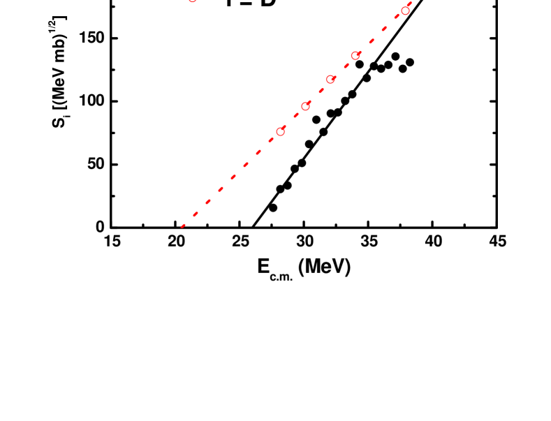
Fig. 1: The Stelson plot of $S_{i}=\sqrt{E_{c.m.}\sigma_{i}}$ for DR ($i=D$, open circles) and fusion ($i=F$, solid circles) cross sections. Use is made of the semi-experimental DR cross section for $S_{D}$, while the experimental fusion cross section is employed for $S_{F}$. The intercepts of the straight lines allow us to extract the threshold energies $E_{0,i}$.

In Fig. 1, we present the experimental $S_{F}(E)$ and $S_{D}(E)$. For $S_{D}(E)$, use is made of $\sigma_{D}^{semi-exp}$. For both $i=F$ and $D$, $S_{i}$ are very well approximated by straight lines in the subbarrier region and thus $E_{0,i}$ can be extracted without much ambiguity. From the zeros of $S_{i}(E)$, one can deduce $E_{0,D}^{semi-exp}$=20.5 MeV and $E_{0,F}^{exp}=$26.0 MeV in the c.m. system. It is interesting to note that $E_{0,D}^{semi-exp}$ is found to be considerably smaller than $E_{0,F}^{exp}$, meaning that the DR channels open at lower energies than fusion channels, which seems physically reasonable.

$E_{0,i}$ may then be used as the energy where the imaginary potential $W_{i}(E)$ becomes zero, i.e., $W_{i}(E_{0,i})=0$ kim1 ; kim2 . This procedure will be used later in the next subsection for obtaining a mathematical expression for $W_{i}(E)$.

III.4 $\chi^{2}$ Analyses

All the $\chi^{2}$ analyses performed in the present work are carried out by using the folding potential as the bare potential $V_{0}(r)$ described in III.B and by using the polarization potentials with fixed geometrical parameters, $r_{F}$=1.40 fm, $a_{F}$=0.43 fm, $r_{D}$=1.47 fm, and $a_{D}$=0.58 fm, which are close to the values used in our previous study kim1 . Some changes of the values from those of Ref. kim1 were made to improve the $\chi^{2}$-fitting.

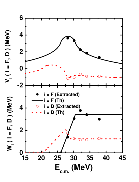
Fig. 2:  The strength parameters $V_{i}$ (upper panel) and $W_{i}$ (lower panel) for $i=D$ and $F$ as functions of $E_{c.m.}$. The open and the solid circles are the strength parameters for $i=D$ and $F$, respectively. The dotted and the solid lines in the lower panel denote $W_{D}$ and $W_{F}$ from Eqs. (13) and (14), respectively, while the dotted and the solid curves in the upper panel represent $V_{D}$ and $V_{F}$ calculated by using the dispersion relation of Eq. (5). The potential values and the corresponding reference energies are such that $V_{F}$ ($E_{s}$ = 30.5 MeV) = 3.1 MeV and $V_{D}$ ($E_{s}$ = 27.5 MeV) = -0.6 MeV, respectively.

As in Ref. kim1 , the $\chi^{2}$ analyses are done in two steps; in the first step, all 4 strength parameters, $V_{F}(E)$, $W_{F}(E)$, $V_{D}(E)$ and $W_{D}(E)$ are varied. In this first step, we can fix fairly well the strength parameters of the DR potential, $V_{D}(E)$ and $W_{D}(E)$, in the sense that $V_{D}(E)$ and $W_{D}(E)$ are determined as smooth functions of $E$. The values of $V_{D}(E)$ and $W_{D}(E)$ thus extracted are presented in Fig. 2 by open circles. The values of $W_{D}(E)$ thus extracted can be well represented by the following function of $E(=E_{c.m.})$ (in units of MeV)

$$W_{D}(E)\;=\;\left\{\begin{array}[]{lll}0&\;\;\mbox{for $E\leq E_{0,D}^{semi-exp}=$20.5}\\ 0.300(E-20.5)&\;\;\mbox{for 20.5$<E\leq$27.5}\\ -0.567(E-27.5)+2.10&\;\;\mbox{for 27.5$<E\leq$29.0}\\ 1.25&\;\;\mbox{for 29.0$<E$}\\ \end{array}\right.\vspace{2ex}$$ (13)

Note that the threshold energies where $W_{D}(E)$ becomes zero are set equal to $E_{0,D}^{semi-exp}$ as determined in the previous subsection and are also indicated by the open circles at $E=20.5$ MeV in Fig. 2. The dotted line in the lower panel of Fig. 2 represents Eq. (13). The dotted curve in the upper panel of Fig. 2 denotes $V_{D}$ as predicted by the dispersion relation of Eq. (5), with $W_{D}(E)$ given by Eq. (13). As seen, the dotted curves reproduce the open circles fairly well, indicating that $V_{D}(E)$ and $W_{D}(E)$ extracted by the $\chi^{2}$ analyses satisfy the dispersion relation.

In this first step of $\chi^{2}$ fitting, however, the values of $V_{F}(E)$ and $W_{F}(E)$ are not reliably fixed in the sense that the extracted values fluctuate considerably as functions of $E$. This is understandable from the expectation that the elastic scattering data can probe most accurately the optical potential in the peripheral region, which is nothing but the region characterized by the DR potential. The part of the nuclear potential responsible for fusion is thus difficult to pin down in this first step.

In order to obtain more reliable information on $V_{F}$ and $W_{F}$, we thus have performed the second step of the $\chi^{2}$ analysis; this time, instead of doing a 4-parameter search we fix $V_{D}$ and $W_{D}$ as determined by the first $\chi^{2}$ fitting, i.e., $W_{D}(E)$ given by Eq. (13) and $V_{D}(E)$ predicted by the dispersion relation. We then perform 2-parameter $\chi^{2}$ analyses, treating only $V_{F}(E)$ and $W_{F}(E)$ as adjustable parameters. The values thus determined are presented in Fig. 2 by the solid circles. As seen, both $V_{F}(E)$ and $W_{F}(E)$ are determined to be fairly smooth functions of $E$. The $W_{F}(E)$ values may be represented by

$$W_{F}(E)\;=\;\left\{\begin{array}[]{lll}0&\;\;\mbox{for $E\leq E_{0,F}^{exp}=$26.0}\\ 0.756(E-26.0)&\;\;\mbox{for 26.0$<E\leq$30.5}\\ 3.40&\;\;\mbox{for 30.5$<E$}\\ \end{array}\right.\vspace{2ex}$$ (14)

As is done for $W_{D}(E)$, the threshold energy where $W_{F}(E)$ becomes zero is set equal to $E_{0,F}^{exp}$, which is also indicated by the solid circle in Fig. 2. As seen, the $W_{F}(E)$ values determined by the second $\chi^{2}$ analyses can fairly well be represented by the functions given by Eq.(14). Note that the energy variations seen in $W_{F}(E)$ and $V_{F}(E)$ are more pronounced than those in $W_{D}(E)$ and $V_{D}(E)$ and exhibit the threshold anomaly as observed in tightly bound projectiles bae1 ; lil1 ; ful1 .

Using $W_{F}(E)$ given by Eq. (14), one can generate $V_{F}(E)$ from the dispersion relation. The results are shown by the solid curve in the upper panel of Fig. 2, which again well reproduces the values extracted from the $\chi^{2}$-fitting. This means that the fusion potential determined from the present analysis also satisfies the dispersion relation.

III.5 Final Calculated Cross Sections in Comparison with the Data

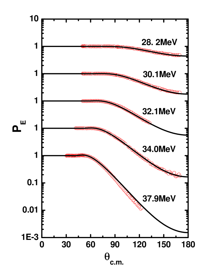
Fig. 3:  Ratios of the elastic scattering cross sections to the Rutherford cross section, $P_{E}$=$\sigma_{E}/\sigma_{R}$, calculated with our final dispersive optical potential are shown in comparison with the experimental data. The data are taken from Ref. kee1 .

Using $W_{D}(E)$ given by Eq. (13) and $W_{F}(E)$ given by Eq. (14) together with $V_{D}(E)$ and $V_{F}(E)$ generated from the dispersion relation, we have performed the final calculations of the elastic, DR and fusion cross sections. The results are presented in Figs. 3 and 4 in comparison with the experimental data. All the data are well reproduced by the calculations.

It may be worth noting here that the theoretical fusion cross section, $\sigma_{F}^{th}$, includes partial contributions, $\sigma_{I}$ and $\sigma_{F}$, from two imaginary components $W_{I}(r)$ and $W_{F}(E)f(X_{F})$ in $U_{F}(r,E)$ given by Eq. (3). In Table 2 the partial contribution from the $W_{I}(r)$ part, denoted by $\sigma_{I}$, are presented in comparison with the total fusion cross section, $\sigma_{F}^{th}$. As seen, the contribution from the inner part, $W_{I}$, amounts to $14\sim 25$ % of $\sigma_{F}^{th}$, which is relatively small but not negligible. It should be remarked, however, that the real potential $V_{I}(r)=V_{I}f(X_{I})$ corresponding to $W_{I}(r)$ does not contribute at all to any cross section if the strength $V_{I}$ is less than, say, 20 MeV. This justifies the fact that we have ignored the $V_{I}(r)$ term.

Table 2: Partial contributions $\sigma_{I}$ and $\sigma_{F}$ in comparison with the total fusion section, $\sigma^{th}_{F}$.

$E_{lab}$	$E_{c.m.}$	$\sigma_{I}$	$\sigma_{F}$	$\sigma^{th}_{F}$
(MeV)	(MeV)	(mb)	(mb)	(mb)
29	28.2	5	16	21
31	30.1	16	92	108
33	32.1	29	180	209
35	34.0	50	270	320
39	37.9	100	439	539

At the moment, there are no data available for the DR cross sections, $\sigma_{D}^{exp}$, which we may compare with our calculated DR cross section $\sigma_{D}^{th}$ of Eq. (7). However, there are some data available; breakup-fusion cross sections (cross sections of breakup of ⁶Li $\longrightarrow\alpha+d$ followed by the absorption of one of the fragments) which is referred to as the incomplete fusion cross section, $\sigma_{ICF}$, in Ref. liu1 and also exclusive $\alpha-d$ and $\alpha-p$ coincidence cross sections sig4 . The sum of these cross sections become fairly large. In Table 3, we present the sum of these cross sections denoted as $\sigma_{ICF+excl}$ in comparison with our theoretical DR cross sections. As seen, $\sigma_{ICF+excl}$ is slightly smaller than $\sigma^{th}_{D}$, which is reasonable, since $\sigma_{ICF+excl}$ does not include such contributions as inelastic excitations of the target nucleus and the incomplete fusion in which only a proton is emitted, and so on. It is thus highly desirable to measure the remaining missing parts of the DR cross sections in the future.

Table 3: Incomplete fusion plus exclusive coincidence cross sections, $\sigma_{ICF+excl}$ in comparison with $\sigma_{D}^{th}$ for the ⁶Li+²⁰⁸Pb system.

$E_{lab}$	$E_{c.m.}$	$\sigma_{ICF+excl}$	$\sigma^{th}_{D}$	$\sigma^{semi-exp}_{D}$
(MeV)	(MeV)	(mb)	(mb)	(mb)
29	28.2		207	205
31	30.1	264	312	306
33	32.1	415	448	430
35	34.0	517	558	545
39	37.9	735	715	778

III.6 Discussions

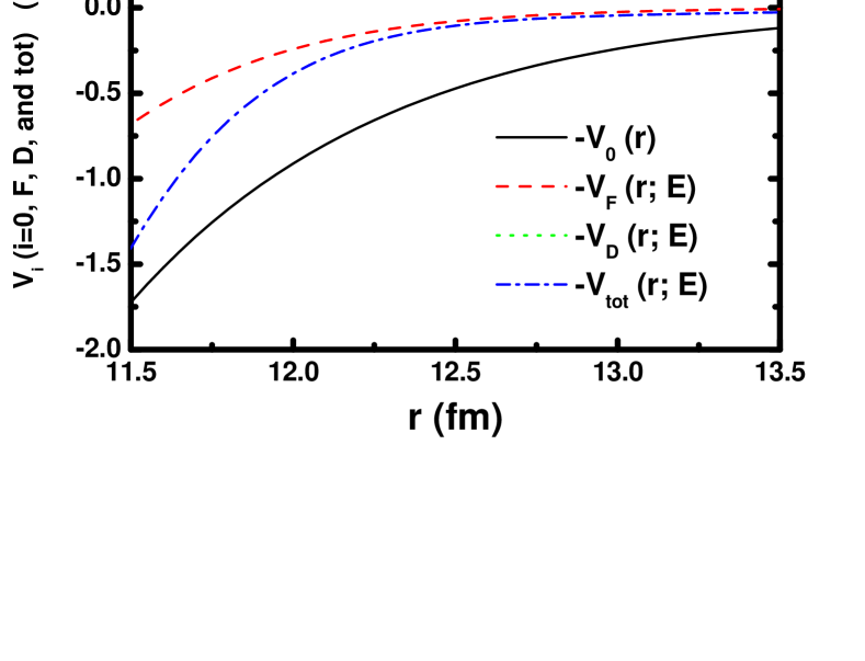
Fig. 5: The double folding potential, real parts of fusion and DR potentials, and the sum of these potentials are plotted for $E_{c.m.}$=28.2 MeV.

It is remarkable that the real part of the DR potentials determined in the present $\chi^{2}$ analysis turn out to be repulsive at all the energies considered here. We present in Fig. 5 the real part of the DR potential, $-V_{D}(r,E)$, at $E_{c.m.}=28.2$ MeV in comparison with the folding potential, $-V_{0}(r)$, in the surface region, $11.5$ fm $<r<13.5$ fm. Also, the real part of the fusion potential, $-V_{F}(r,E)$, and the sum, $-V_{tot}(r,E)$, of all these three potentials are shown. As seen, the values of the sum of real potentials are significantly reduced from those of the bare folding potential.

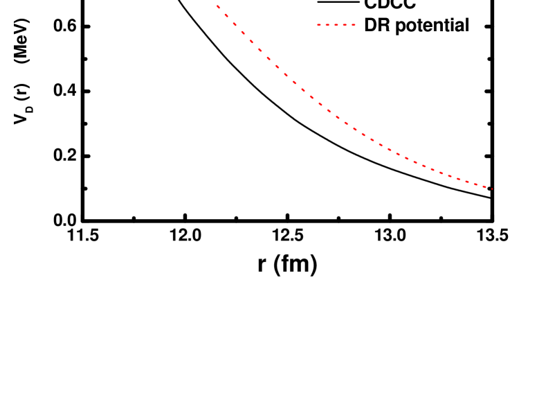
Fig. 6: The real part of the DR potential $V_{D}(r,E)$ is plotted in comparison with that of the polarization potential deduced from the CDCC calculations for ⁶Li+²⁰⁸Pb system at $E_{c.m.}$=28.2 MeV.

It may be interesting to compare our $-V_{D}(r,E)$ with the real part of the polarization potential obtained from the CDCC calculations. Such a comparison is made in Fig. 6, where $-V_{D}(r,E)$ shown in Fig. 5 is compared with the polarization potential calculated at $E_{c.m.}=28.2$ MeV kee2 . As seen, two potentials show similar behaviours and agree qualitatively with each other both in magnitude and in radial dependence. This indicates that the DR potential deduced from the present analyses of the elastic scattering and fusion data describes essentially the same physical effects as treated in the CDCC calculation.

In Table 4 presented are the values of the strong absorption radius $R_{sa}$, and those of $V_{0}$, $V_{F}$, $V_{D}$, $V_{tot}$, $W_{F}$, $W_{D}$, and $R=V_{tot}/V_{0}$ at $r=R_{sa}$ for all the energies considered here. The values of $R_{sa}$ decrease slightly with the incident energy and range from 12.27 fm to 12.75 fm. Note that the value of $R=0.19\sim 0.37$ may be compared with that of 0.51 obtained in Ref. kee2 . (The normalization factor used for the same system at $E_{lab}$ = 50.6 MeV in Ref. sat1 was 0.59.) It is seen also in Table 4 that at the strong absorption radius $R_{sa}$, the values of the real and the imaginary parts of the DR potential are both considerably greater than those of the fusion potential. Because of this, the energy dependence of the net polarization potential (sum of the fusion and DR potentials) at $R_{sa}$ is dominated by that of the DR potential with rather a smooth energy dependency. Consequently, the net potential does not show such a threshold anomaly as seen in the net potential for systems with tightly bound projectiles bae1 ; lil1 ; ful1 .

As already remarked, the real and the imaginary parts of both fusion and DR potentials determined in the present $\chi^{2}$ analyses satisfy well the dispersion relation, and further the fusion potential shows clearly the threshold anomaly.

Table 4: The value of the strong absorption radius, $R_{sa}$, and those of $V_{0}$, $V_{F}$, $V_{D}$, $V_{tot}$, $W_{F}$, $W_{D}$, and $R=V_{tot}/V_{0}$ evaluated at $r=R_{sa}$ for all the energies.

Ec.m.	$R_{sa}$	$-V_{0}$	$-V_{F}$	$-V_{D}$	$-V_{tot}$	$-W_{F}$	$-W_{D}$	$R=V_{tot}/V_{0}$
(MeV)	(fm)	(MeV)	(MeV)	(MeV)	(MeV)	(MeV)	(MeV)
28.2	12.75	-0.338	-0.045	0.318	-0.065	-0.019	-0.539	0.19
30.1	12.56	-0.436	-0.061	0.334	-0.163	-0.056	-0.512	0.37
32.1	12.46	-0.499	-0.051	0.382	-0.168	-0.077	-0.583	0.34
34.0	12.39	-0.547	-0.047	0.437	-0.157	-0.090	-0.635	0.29
37.9	12.27	-0.641	-0.042	0.553	-0.130	-0.118	-0.730	0.20

IV Conclusions

From the discussions of our results in the previous section, we may safely conclude that within the extended optical model approach, even if use is made of the double folding potential as its bare potential, one can describe the elastic scattering and fusion cross section data simultaneously without encountering the two problems remarked at the beginning of this paper. The normalization factor needed to be introduced to the folding potential, particularly for loosely bound projectiles, in the earlier analyses sat1 ; kee1 based on the conventional optical model approach can now be removed in the present extended optical model analysis, and the effects are accounted for by means of the repulsive DR potential as observed in the CDCC approach. Also the threshold anomaly that could not be seen in the analyses based on the conventional optical model approach is now seen in the fusion part of the polarization potential.

In the present work, we focused our attention only to the ⁶Li+²⁰⁸Pb system, but it is possible to carry out similar analyses to other systems. It is particularly interesting to do the analysis for the ⁷Li+²⁰⁸Pb system, where the conventional analysis is successfully applied to explain the data. An extension of the present analysis to the ⁷Li+²⁰⁸Pb system is now under way, and the report of the results will be made in a separated paper.

This work was supported by the Korea Research Foundation Grant funded by the Korean Government (MOEHRD) (KRF- 2006-214-C00014).

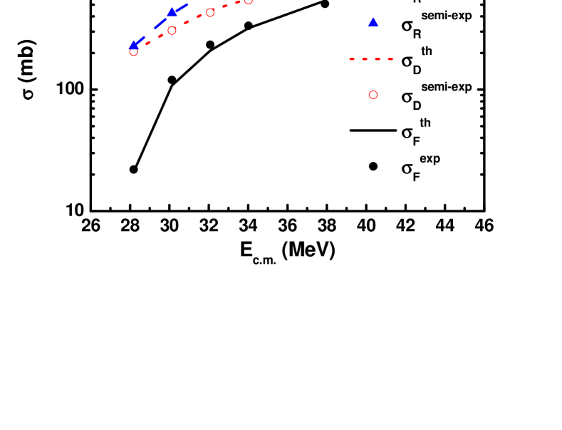
Fig. 4:  DR and fusion cross sections calculated with our final dispersive optical potential are shown in comparison with the experimental data. $\sigma_{R}^{semi-exp}$ and $\sigma_{D}^{semi-exp}$ denoted by the triangles and the open circles, respectively, are obtained as described in Sec.II. The fusion data are from Ref. wu1 .

References

- (1)
- (2) G. R. Satchler and W. G. Love, Phys. Rep. 55, 183 (1979).
- (3) N. Keeley, S. J. Bennett, N. M. Clarke, B. R. Fulton, G. Tungate, P. V. Drumm, M. A. Nagarajan, and J. S. Lilly, Nucl. Phys. A571, 326 (1994).
- (4) C. C. Mahaux, H. Ngo, and G. R. Satchler, Nucl. Phys. A449, 354 (1986); Nucl. Phys. A456, 134 (1986).
- (5) M. A. Nagarajan, C. C. Mahaux, and G. R. Satchler, Phys. Rev. Lett. 54, 1136 (1985).
- (6) Y. Sakuragi, Phys. Rev. C 35, 2161 (1987).
- (7) N. Keeley and K. Rusek, Phys. Lett. B 427, 1 (1998).
- (8) T. Udagawa, M. Naito, and B. T. Kim, Phys. Rev. C 45, 876 (1992).
- (9) B. T. Kim, W. Y. So, S. W. Hong, and T. Udagawa, Phys. Rev. C 65, 044616 (2002).
- (10) W. Y. So, S. W. Hong, B. T. Kim, and T. Udagawa, Phys. Rev. C 69, 064606 (2004).
- (11) E. F. Aguilera, J. J. Kolata, F. D. Becchetti, P. A. DeYoung, J. D. Hinnefeld, A. Horvath, L. O. Lamm, Hye-Young Lee, D. Lizcano, E. Martinez-Quiroz, P. Mohr, T. W. O’Donnell, D. A. Roberts, and G. Rogachev, Phys. Rev. C 63, 061603(R) (2001).
- (12) J. J. Kolata, V. Guimarães, D. Peterson, P. Santi, R. White-Stevens, P. A. DeYoung, G. F. Peaslee, B. Hughey, B. Atalla, M. Kern, P. L. Jolivette, J. A. Zimmerman, M. Y. Lee, F. D. Becchetti, E. F. Aguilera, E. Martinez-Quiroz, and J. D. Hinnefeld, Phys. Rev. Lett. 81, 4580 (1998).
- (13) E. F. Aguilera, J. J. Kolata, F. M. Nunes, F. D. Becchetti, P. A. DeYoung, M. Goupell, V. Guimaraes, B. Hughey, M. Y. Lee, D. Lizcano, E. Martinez-Quiroz, A. Nowlin, T. W. O’Donnell, G. F.Peaslee, D. Peterson, P. Santi, and R. White-Stevens, Phys. Rev. Lett. 84, 5058 (2000).
- (14) Y. W. Wu, Z. H. Liu, C. J. Lin, H. Q. Zhang, M. Ruan, F. Yang, Z. C. Li, M. Trotta, and K. Hagino, Phys. Rev. C. 68, 044605 (2003).
- (15) M. Dasgupta, D. J. Hinde, K. Hagino, S. B. Moraes, P. R. S. Gomes, R. M. Anjos, R. D. Butt, A. C. Berriman, N. Carlin, C. R. Morton, J. O. Newton, and A. Szanto de Toledo, Phys. Rev. C 66, 041602(R) (2002).
- (16) C. Signorini, A. Andrighetto, M. Ruan, J. Y. Guo, L. Stroe, F. Soramel, K. E. G. Löbner, L. Müller, D. Pierroutsakou, M. Romoli, K. Rudolph, I. J. Thompson, M. Trotta, A. Vitturi, R. Gernhäuser, and A. Kastenmüller, Phys. Rev. C 61, 061603(R) (2000).
- (17) C. Signorini, Z. H. Liu, Z. C. Li, K. E. G. Löbner, L. Müller, M. Ruan, K. Rudolph, F. Soramel, C. Zotti, A. Andrighetto, L. Stroe, A. Vitturi, H. Q. Zhang, Eur. Phys. J. A 5, 7 (1999) and private communications.
- (18) T. Udagawa, B. T. Kim, and T. Tamura, Phys. Rev. C 32, 124 (1985); T. Udagawa and T. Tamura, Phys. Rev. C 29, 1922 (1984).
- (19) S.-W. Hong, T. Udagawa, and T. Tamura, Nucl. Phys. A491, 492 (1989).
- (20) T. Udagawa, T. Tamura, and B. T. Kim, Phys. Rev. C 39, 1840 (1989); B. T. Kim, M. Naito, and T. Udagawa, Phys. Lett. B 237, 19 (1990).
- (21) A. Baeza, B. Bilwes, J. Diaz, and J. L. Ferrero, Nucl. Phys. A419, 412 (1984).
- (22) J. S. Lilley, B. R. Fulton, M. A. Nagarajan, I. J. Thompson, and D. W. Banes, Phys. Lett. 151B, 181 (1985).
- (23) B. R. Fulton, D. W. Banes, J. S. Lilley, M. A. Nagarajan, and I. J. Thompson, Phys. Lett. 162B, 55 (1985).
- (24) C. Signorini, M. Mazzocco, G. F. Prete, F. Soramel, L. Stroe, A. Andrighetto, I. J. Thompson, A. Vitturi, A. Brondi, M. Cinausero, D. Fabris, E. Fioretto, N. Gelli, J. Y. Guo, G. La Rana, Z. H. Liu, F. Lucarelli, R. Moro, G. Nebbia, M. Trotta, E. Vardaci, and G. Viesti, Eur. Phys. J. A 10, 249 (2001).
- (25) C. Signorini, A. Edifizi, M. Mazzocco, M. Lunardon, D. Fabris, A. Vitturi, P. Scopel, F. Soramel, L. Stroe, G. Prete, E. Fioretto, M. Cinausero, M. Trotta, A. Brondi, R. Moro, G. La Rana, E. Vardaci, A. Ordine, G. Inglima, M. La Commara, D. Pierroutsakou, M. Romoli, M. Sandoli, A. Diaz-Torres, I. J. Thompson, Z. H. Liu, Phys. Rev. C 67, 044607 (2003).
- (26) C. Signorini, T. Glodariu, Z. H. Liu, M. Mazzocco, M. Ruan, and F. Soramel, Prog. Theor. Phys. Suppl. 154, 272 (2004).
- (27) Z.H. Liu, C. Signorini, M. Mazzocco, M. Ruan, H.Q. Zhang, T. Glodariu, Y.W. Wu, F. Soramel, C.J. Lin, and F. Yang, Eur. Phys. J. A 26, 73 (2005)
- (28) M. Dasgupta, P. R. S. Gomes, D. J. Hinde, S. B. Moraes, R. M. Anjos, A. C. Berriman, R. D. Butt, N. Carlin, J. Lubian, C. R. Morton, J. O. Newton, and A. Szanto de Toledo, Phys. Rev. C 70, 024606 (2004).
- (29) R. H. McCamis, N. E. Davison, W. T. H. van Oers, R. F. Carlson, and A. J. Cox, Can. J. Phys. 64, 685 (1986)
- (30) T. Eliyakut-Roshko, R. H. McCamis, W. T. H. van Oers, R. F. Carlson, and A. J. Cox, Phys. Rev. C 51, 1295 (1995).
- (31) A. Auce, R. F. Carlson, A. J. Cox, A. Ingemarsson, R. Johansson, P. U. Renberg, O. Sundberg, and G. Tibell, Phys. Rev. C 53, 2919 (1996).
- (32) P. Singh, A. Chatterjee, S. K. Gupta, and S. S. Kerekatte, Phys. Rev. C. 43, 1867 (1991).
- (33) C. Y. Wong, Phys. Rev. Lett. 31, 766 (1973).
- (34) W. G. Love, T. Terasawa, and G. R. Satchler, Nucl. Phys. A 291, 183 (1977).
- (35) M. S. Hussein, Phys. Rev. C 30, 1962 (1984).
- (36) C. W. De Jager, H. DeVries, and C. DeVries, Atomic Data and Nuclear Data Tables, 14, 479 (1974).
- (37) J. Cook, Comp. Phys. Comm. 25, 125 (1982).
- (38) P. H. Stelson, Phys. Lett. B 205, 190 (1988); P. H. Stelson, H. J. Kim, M. Beckerman, D. Shapira, and R. L. Robinson, Phys. Rev. C 41, 1584 (1990).
- (39) B. T. Kim, W. Y. So, S. W. Hong, and T. Udagawa, Phys. Rev. C. 65, 044607 (2002).