Shell-model study of spectroscopies and isospin structures in odd-odd $N=Z$ nuclei employing realistic NN potentials

Abstract

The structures of odd-odd $N=Z$ nuclei in the lower fp shell have been investigated with a new isospin-nonconserving microscopical interaction. The interaction is derived from a high-precision charge-dependent Bonn nucleon-nucleon potential using the folded-diagram renormalization method. Excellent agreements with experimental data have been obtained up to band terminations. Particularly, the relative positions of $T=0$ and $T=1$ bands were well reproduced. Calculations with another interaction obtained from the Idaho-A chiral potential showed similar results. Our calculations also give a good description of the existence of high-spin isomeric states in the $0f_{7/2}$ sub-shell. As examples, the spectroscopies and isospin structures of ⁴⁶V and ⁵⁰Mn have been discussed in detail, with the useful predictions of level structures including electromagnetic properties. Results for ⁵⁰Mn were analyzed where experimental observations are still insufficient.

I Introduction

Nuclei with the equal numbers of neutrons and protons ($N=Z$) have become a special ground to investigate neutron-proton (np) correlations. In $N=Z$ nuclei, neutrons and protons occupy the same shell-model orbits, leading to large spatial overlaps between neutron and proton wave functions. The np pairing is further enhanced in odd-odd $N=Z$ nuclei due to odd neutron and odd proton correlation. The np residual pairing interaction can be equally important as the neutron-neutron (nn, $T_{z}=1,T=1$) and proton-proton (pp, $T_{z}=-1,T=1$) pairings. While nn and pp pairings have been well established in terms of the simple BCS model, the np pairing is still an open question that has motivated many recent theoretical and experimental works Dean03 ; Schneider99 ; Poves98 ; Fries98 ; Schmidt00 ; Oleary02 ; Brandolini01 ; Brentano01 ; Pietralla02 ; Svensson98 ; Sko98 ; Lenzi99 ; OLeary99 ; Faes99 ; Satula01 ; Macchiavelli ; Vogel00 ; Janecke05 .

In contrast to pp and nn correlations, the np pairing can form isovector ($T_{z}=0,T=1$) and isoscalar ($T_{z}=0,T=0$) configurations. The isovector channel manifest itself in a similar fashion to like-nucleon correlations, which can be evidenced with the presence of nearly degenerate $T=1$ isobaric triplets along the $N=Z$ line Macchiavelli . The existence of the $T=0$ isoscalar component has also been shown theoretically, e.g., in Ref. Satula01 . In light $N=Z$ nuclei, ground states usually favor the lowest $T=0$ isospin quantum number, while $T=1$ states appear at very high excitation energies. With increasing mass number, however, $T=0$ and $T=1$ bands begin to coexist at low excitation energies Dean03 ; Janecke05 . In particular, the isospin structures of medium-mass fp shell nuclei are very interesting, where $T=1$ states can be lower than $T=0$ states. $T=1$ ground states have been expected systematically Janecke05 ; Vogel00 .

Recent advances in experimental techniques enable us to study the structures of the odd-odd $N=Z$ nuclei in the fp shell at high spins and high excitation energies. This provides an unique opportunity to investigate the interplay between $T=0$ and $T=1$ bands. Moreover, the high-precision measurements of level schemes provide useful information for discussion of the isospin asymmetry in their excited states at different angular momenta Schneider99 ; Fries98 ; Schmidt00 ; Oleary02 ; Pietralla02 ; Svensson98 ; Sko98 ; Lenzi99 ; OLeary99 ; Faes99 . Experimentally, isospin effects can be discussed by defining the mirror energy differences (MED) and triplet energy differences (TED) between analogous states in mirror pairs and $T=1$ triplets, respectively Lenzi01 ; Garrett01 ; Zuker02 . The differences have their origins from the Coulomb interaction and charge dependence in strong force, while the former usually plays a dominant role. In the fp shell, the coulomb shifts of single-particle orbits are relatively small Zuker02 . This allows us to extract the effect from the charge symmetry breaking in the strong force for the many-body systems of nuclei.

The purpose of this paper is to study the structures and properties of odd-odd $N=Z$ nuclei in the fp model space by the shell-model diagonalization method. The many-body interaction used in the effective Hamiltonian has been derived from a high-precision charge-dependent Bonn (CD-Bonn) nucleon-nucleon (NN) potential Machleidt01 using the so-called folded-diagram method Kuo90 . The obtained interaction retains the charge-independence breaking effects in the NN potential. The contribution from the Coulomb field is also included. Hence the effective Hamiltonian does not conserve isospin.

In Section II, we describe briefly the folded-diagram method and the construction of the residual interaction. In Section III, the level structures of the odd-odd $N=Z$ nuclei in the $fp$ shell are calculated and discussed. In Section IV, we discuss the electromagnetic properties of the odd-odd $N=Z$ nuclei with analyzing the isospin structures of the nuclei.

II Effective interaction

We start from the mean-field approximation with the perturbation expansion. In this approximation, it is convenient to reduce the degree of freedom of the Hilbert space for the many-fermion system of nuclei. For large-scale shell-model diagonalizations, the determination of the model space is a crucial step. The model space can be defined with the projection operator,

$$P=\sum_{i=1}^{D}|\Phi_{i}\rangle\langle\Phi_{i}|,$$ (1)

where $D$ is the dimension of the model space, and wave functions $|\Phi_{i}\rangle$ are eigenfunctions of the unperturbed Hamiltonian, $H_{0}=T+U$, with $T$ being the kinetic energy and $U$ an appropriate one-body potential. The remaining space (so-called excluded space) can be expressed by

$$Q=\sum_{i=D+1}^{\infty}|\Phi_{i}\rangle\langle\Phi_{i}|.$$ (2)

The system of the full Hamiltonian with eigen energies $E_{\alpha}$ and wave functions $\Psi_{\alpha}$ that are determined by the full Schrödinger equation of $H|\Psi_{\alpha}\rangle=E_{\alpha}|\Psi_{\alpha}\rangle$ can be reduced within the model space by projection Kuo90 ,

$$PH_{\text{eff}}P|\Psi_{\lambda}\rangle=(E_{\lambda}-E_{c})P|\Psi_{\lambda}\rangle=(E_{\lambda}-E_{c})|\Phi_{\lambda}\rangle,$$ (3)

with $E_{\lambda}\in\{E_{\alpha}\}~{}(\lambda=1,2,\cdots,D)$ and $E_{c}$ is the energy of the assumed core left behind in practical calculations. $H_{\text{eff}}$ is the mode-space-dependent effective Hamiltonian. In the shell model context, the effective Hamiltonian can be decomposed into two parts,

$$H_{\text{eff}}=H_{\text{0}}^{\prime}+v_{\text{eff}},$$ (4)

where $H_{\text{0}}^{\prime}=\sum_{\alpha}\varepsilon_{\alpha}^{\prime}\text{a}^{{\dagger}}_{\alpha}\text{a}_{\alpha}$ is the effective one-body Hamiltonian with $\varepsilon_{\alpha}^{\prime}$ being single-particle energies (SPE). The $\varepsilon_{\alpha}^{\prime}$ values can be obtained from the separation energies of valence particles. Usually, the effective interaction $v_{\text{eff}}$ takes the form of pure two-body interactions. It can be expressed as two body matrix elements in harmonic oscillator (HO) basis.

The shell model provides the microscopic foundation to study the excitations of nuclei. The Cohen-Kurath ck and universal SD (USD) USD interactions have been proved to be quite successful and useful for the $p$- and $sd$- shell calculations, respectively. In past decades, extensive theoretical works have been conducted to improve the calculations of the shell model for $0f_{7/2}$ nuclei in which exact diagonalizations have become possible due to the advance in computing techniques. The central spirit of shell model calculations is to find a unified interaction for a given mass region. For the fp nuclei, various interactions have been proposed, such as the Kuo-Brown (KB) renormalized G matrix Kuo68 and its modified versions with monopole centroid corrections KB3 ; Caurier05 , the FPD6 analytic two-body potential Richter91 and the GXPF interaction Honma02 . These interactions have been extensively tested with the successful descriptions of rotational collectivities of nuclei in the upper part of the $0f_{7/2}$ shell (e.g., ⁴⁸Cr) Caurier94 ; Caurier95 ; MPinedo96a . However, these interactions conserve isospin symmetry. In this work, we present a new isospin-nonconserving effective interaction derived microscopically from the underlying $NN$ potential.

Traditionally, effective residual interaction is derived from phenomenal fit to observations USD (e.g., the USD interaction for the $sd$ shell.) or from the evaluation of the G reaction matrix Caurier05 . Although the effective interaction can in principle be derived from true $NN$ interaction, it has to be renormalized to include the contributions from the excluded configurations and to avoid the hard core of the bare $NN$ potential. Renormalization methods have been proposed for the calculation of effective interaction from underlying meson-exchange potentials, like the momentum-space renormalization group decimation method ($V_{\text{low-}k}$ approach) Bogner03 and the unitary correlation operator method (UCOM) Feldmeier98 . In $V_{\text{low-}k}$ approach, high-momentum contributions are integrated out with the introduction of a cutoff, while UCOM describes short-range correlations by a unitary transformation. In this paper, we used the so-called folded-diagram expansion method in which it is more convenient to include effects from excluded configurations. The folded-diagram expansion is a time-dependent perturbation theory introduced by Kuo et al. for the evaluation of residual interactions microscopically from bare NN potentials Kuo90 ; Jensen95 . The short-range repulsion is taken into account by the introduction of G matrix.

The folded (time-incorrect) and non-folded (time-correct) diagrams are introduced in the evaluation of the time-evolution operator U$(0,-\infty)$ which can be written using perturbation expansion in the complex-time limit as,

$$\text{U}(0,-\infty)=\lim_{t\rightarrow-\infty(\varepsilon)}\sum_{n=0}^{\infty}\frac{1}{n!}(\frac{-\text{i}}{\hbar})^{n}\int_{t}^{0}\text{d}t_{1}\int_{t}^{0}\text{d}t_{2}\cdots\int_{t}^{0}\text{d}t_{n}T[H_{1}(t_{1}),H_{1}(t_{2})\cdots H_{1}(t_{n})],$$ (5)

where $\lim_{t\rightarrow-\infty(\varepsilon)}\equiv\lim_{\varepsilon\rightarrow 0^{+}}\lim_{t\rightarrow-\infty(1-\text{i}\varepsilon)}$ and T is the time-ordering operator in degenerate or nearly degenerate systems. For a model-space with the dimension $D$, the lowest $D$ eigenstates of the true Hamiltonian can be constructed using the time-evolution operator with model-space states, $\Phi_{i}$,

$$\lim_{t\rightarrow-\infty(\varepsilon)}\frac{\text{U}(0,-\infty)|\rho_{\lambda}\rangle}{\langle\rho_{\lambda}|\text{U}(0,-\infty)|\rho_{\lambda}\rangle}=\frac{|\Psi_{\lambda}\rangle}{\langle\rho_{\lambda}|\Psi_{\lambda}\rangle},$$ (6)

where $\lambda=1,2,\cdots,D$ and $|\rho_{\lambda}\rangle$ is a set of $D$ parent states defined as

$$|\rho_{\lambda}\rangle=\sum_{i=1}^{D}C_{i}^{(\lambda)}|\Phi_{i}\rangle,~{}~{}~{}~{}~{}\lambda=1,2,\cdots,D.$$ (7)

In the folded-diagram decomposition procedure, the wave function $\text{U}(0,-\infty)|\Phi_{i}\rangle$ can be factorized as

$$\text{U}(0,-\infty)|\Phi_{i}\rangle=\text{U}_{V}(0,-\infty)|\Phi_{i}\rangle\times\text{U}(0,-\infty)|c\rangle,$$ (8)

where $|c\rangle$ denotes the core and the subscript V means that all interactions in $\text{U}_{V}(0,-\infty)$ are linked to valence particles. Moreover, diagrams contained in $\text{U}_{V}(0,-\infty)|\Phi_{i}\rangle$ can be expressed in terms of so-called $\hat{Q}$-boxes. The $\hat{Q}$-box is made up of non-folded diagrams which are irreducible and valence-linked Kuo90 . It is defined as

$$\hat{Q}(\omega)=PH_{1}P+PH_{1}\mathcal{Q}\frac{1}{\omega-\mathcal{Q}H\mathcal{Q}}\mathcal{Q}H_{1}P,$$ (9)

where $\omega$ is the energy of interacting nucleons. The exclusion operator $\mathcal{Q}$ appears due to the Pauli principle preventing interacting nucleons from scattering into states occupied already by other nucleons Jensen95 .

Using the generalized time ordering, the effective interaction $v_{\text{eff}}$ can be expanded in terms of $\hat{Q}$-boxes:

$$v_{\text{eff}}=\hat{Q}-\hat{Q}^{\prime}\int\hat{Q}+\hat{Q}^{\prime}\int\hat{Q}\int\hat{Q}-\cdots,$$ (10)

where $\int$ denotes a folding sign imposing relative time constraints. $\hat{Q}^{\prime}$ is a set of $\hat{Q}$-boxes that have at least two $H_{1}$ vertices attached to valence lines, satisfying $\text{d}\hat{Q}^{\prime}/\text{d}\omega=\text{d}\hat{Q}/\text{d}\omega$. Correspondingly, the solution of Eq. (10) can be derived using an iteration procedure:

$$v_{\text{eff}}^{(n)}=\hat{Q}+\sum_{m=1}^{\infty}\frac{1}{m!}\frac{d^{m}\hat{Q}}{d\omega^{m}}\{v_{\text{eff}}^{(n-1)}\}^{m},$$ (11)

where the energy dependence of the $\hat{Q}$-box can be removed.

In practical evaluations, non-folded diagrams are calculated firstly and summed to give the $\hat{Q}$-box. To treat the strong repulsive core of the bare $NN$ potential which is unsuitable for perturbation treatments, the Brueckner $G$ reaction matrix is usually used. The $\hat{Q}$-boxes can be expressed in terms of G-matrix vertices. The $G$ matrix is defined by the solution of the Bethe-Goldstone equation Jensen95 ,

$$G=V+V\frac{\mathcal{Q}}{\omega-\mathcal{Q}H_{0}\mathcal{Q}}G,$$ (12)

satisfying

$$\langle\Psi|G|\Psi\rangle=\langle\Psi|V|\Psi\rangle,$$ (13)

where $\Psi$ is the correlated two-body wave function.

In the past decade, various high-precision phenomenological meson-exchange potentials have been proposed with reasonable descriptions of the charge symmetry breaking and charge independence breaking Machleidt01 . Initiated by Weinberg Entem03 , the chiral perturbative NN potential derived from the low energy effective Lagrangians of the QCD model shows another promising way. All the potentials have similar low-momentum behavior. In the present work, the bare $NN$ potential $V$ is taken to be a new charge-dependent version of the Bonn one-boson-exchange potential as described in Ref. Machleidt01 . For further studies, theoretical works have also been carried out with a N²LO chiral NN potential by Idaho group Entem03 .

In the present work, we are interested in nuclei in the fp shell. The model space contains $0f_{7/2},~{}1p_{3/2},~{}0f_{5/2},~{}1p_{1/2}$ sub-shells with the core of ⁴⁰Ca. The $\hat{Q}$-boxes are approximated to the third order. Single-particle energies are taken from the experimental excitation energies of the odd neutron in ⁴¹Ca Kuo68 . In the CD Bonn potential, charge symmetry breaking ($V_{pp}\neq V_{nn}$) and charge independence breaking ($V_{pp}\neq V_{pn}\neq V_{nn}$) effects are embedded in all partial waves with angular momentum $J\leq 4$. The contribution from the Coulomb field is also added when calculating the G matrix. The derived interaction is composed of three parts: the proton-proton, neutron-neutron and proton-neutron interactions. No specific mass dependence of the interaction is considered.

III level structure

We calculated the level structures of odd-odd $N=Z$ nuclei in the lower part of fp shell with the residual interaction derived as above. The effective Hamiltonian is diagonalized with the shell-model code OXBASH Oxbash ; Brown01 . The Hamiltonian matrix is given in proton/neutron formalism, with the neutrons and protons being naturally treated as two kinds of particles.

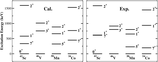
Figure 1: Low-lying states in odd-odd $N=Z$ nuclei in the $0f_{7/2}$ shell. Calculated results and experimental data toi98 are shown on the left-hand and right-hand side, respectively. All $0^{+}$ ground states have the isospin of $T=1$. The $2^{+}$ levels shown are the first excited $T=1$ states.

The calculations of low-lying states in odd-odd $N=Z$ nuclei are shown in Fig. 1. For nuclei with mass number $A\geq 50$, calculations have been done in truncated fp model spaces. While the $0^{+}$ and $2^{+}$ states have $T=1$, other states shown in Fig. 1 have $T=0$. Isospin is not an explicit quantum number in our system. For a given state, the isospin quantum number is assigned through the detailed comparison with neighboring ($T_{z}=\pm 1$) nuclei. Odd-odd $N=Z$ nucleus and neighboring $|T_{z}|=1$ nuclei can form isospin triplet, leading to nearly identical $T=1$ bands. It can be seen that our calculations reproduce well the relative positions of the $T=1$ and $T=0$ states. The largest discrepancy compared with experiments is seen for the $7^{+}_{1}$ state in ⁴²Sc where the core breaking effect that are not taken into account may be non-negligible. For the next heavier odd-odd $N=Z$ nucleus, ⁵⁸Cu, our calculation can reproduce well the near degenerating $T=1$ and $T=0$ bands, which are not shown in the figure. For heavier odd-odd $N=Z$ nuclei, e.g. ⁶²Ga, contributions from the $0g_{9/2}$ sub-shell may become significant.

For comparison, we also used an interaction derived from the Idaho-A chiral $NN$ potential Entem03 to calculate the low-lying states of the nuclei in Fig. 1. Similar results are obtained except ⁴²Sc in which the calculated $7^{+}$ state ($T=0$) is lower than the $0^{+}$ state by about 47 keV in the Idaho-A potential.

As mentioned before, for nuclei in $0f_{7/2}$ shell and above, $T=1$ ground states exist systematically. This situation has been studied by Satuła and Wyss Satula01 with an extended mean-field model in which the $T=1$ configuration is generated by isospin cranking. Based on the analysis of symmetry energy coefficients, the possible existence of isospin inversion has been extended to $A=96$ by Jänecke and O’Donnell Janecke05 . In the shell-model Hamiltonian, different components of two-body interactions are mixed up. It is not easy to identify the role played by each component. One possible way is to separate contributions from so-called isovector and isoscalar pairing terms of the shell-model effective interaction Poves98 . Such an effort has already been tried Poves98 . In Ref. Poves98 , authors argued that in the $0f_{7/2}$ shell the competition between the isovector and isoscalar terms can lower the centroid of the $T=1$ state, leading to a $T=1$ ground state. The shell model could provide an efficient and qualitative way to search the interplay between various pairing correlations on the isospin structures of self-conjugate nuclei. The detailed evaluations of these terms would be done in future.

Tentative calculations have also been done for light nuclei in the $p$- and $sd$- shell. Results for odd-odd $N=Z$ nuclei in these shells are encouraging, showing that the folded-diagram method is valid and efficient for the evaluation of shell-model interaction from NN potentials. It has long been a challenging problem that previous realistic shell-model calculations cannot give the right $3^{+}$ ground state in odd-odd $N=Z$ nuclei ${}^{10}_{~{}5}$B Caurier05 . Our calculations in the psd shell with the CD-Bonn potential reproduce well the $3^{+}$ ground state and other low-lying states.

Experiments have observed high-spin states in ⁴⁶V and ⁵⁰Mn up to the $0f_{7/2}$ band termination Schmidt00 ; Oleary02 ; OLeary99 ; Svensson98 . Our calculations give excellent agreement with experiments. Fig. 2 shows the calculated level scheme for ⁴⁶V. Comparisons with experiments OLeary99 ; Garrett01 for $T=0$ and $T=1$ yrast bands are given in Fig. 3. The ground-state band has been assigned with the quantum number of $K^{\pi}=3^{+}$ and $T=0$ Oleary02 . Recent experiments have deduced the $T=1$ ground-state bands in ⁴⁶V and its isospin-triplet partners, ⁴⁶Ti and ⁴⁶Cr, up to $J^{\pi}=10^{+}$ Garrett01 . Our calculations can reproduce the observations for the $T=1$ ground-state bands of these three nuclei. In ⁴⁶V, a state with the excitation energy of $E=8267$ keV was detected and tentatively assigned as $12^{+}$ by Garrett et al. Garrett01 . The state corresponds to our calculated $12^{+}_{3}$ state with the energy of 8309 keV in which the isospin quantum number was assigned as $T=1$.

Figure 2: Calculated level scheme in ⁴⁶V. The comparison with experimental observations is shown in Fig. 3.

For the next heavier $N=Z$ nucleus, ⁵⁰Mn, we chose a truncation by allowing a maximum of two particles being excited to higher sub-shells above the $f_{7/2}$ orbit. The truncation is valid since configurations for low-lying states are governed by the $0f_{7/2}$ sub-shell. Fig. 4 gives calculated and experimental positive-parity states in ⁵⁰Mn. The experiment Oleary02 has identified the $T=0$ band up to the $0f_{7/2}$ band termination and the $T=1$ band up to $6^{+}$. The observed $8^{+}$ state at 4874 keV and $10^{+}$ state at 6460 keV were assigned $T=0$ by O’Leary et al. Oleary02 . Our calculations reproduce the $T=0$ and $T=1$ states. $T=1$ states can be selected from the calculations of electrical quadruple (E2) and magnetic dipole (M1) transition properties that will be discussed in the next section.

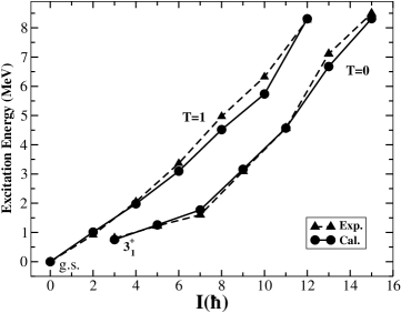
Figure 3: Comparison between calculated and experimental $T=1$ and $T=0$ yrast bands in ⁴⁶V. The experimental data are taken from Refs. OLeary99 ; Garrett01 .

In the framework of the deformed Nilsson diagram, low-energy configurations in ⁵⁰Mn have odd proton and odd neutron occupying the $5/2^{-}[312]$ orbit of the $0f_{7/2}$ sub-shell, leading to low-lying $K^{\pi}=0^{+}$ ($T=0$ or 1) and $K^{\pi}=5^{+}$ ($T=0$) configurations that have been identified experimentally Schmidt00 ; Pietralla02 . Our calculations have well reproduced the observed states, as shown in Fig. 4. Experiments observed that the $K^{\pi}=5^{+}$ state ($T=0$) is a $T_{1/2}=1.75$ m isomer with an excitation energy of 229 keV Schmidt00 ; Pietralla02 . Our calculation gives a energy of 322 keV for the isomer. Its decay is highly hindered due to the $K$ selection rule. Low-lying metastable $T=0$ states also exist in other odd-odd $N=Z$ nuclei shown in Fig. 1, due to large angular momentum gaps between $0^{+}$ ground states and low-lying high-spin states. The $K^{\pi}=0^{+}$ band ($T=0$) in ⁵⁰Mn has been observed with three members of $1^{+}_{1}$, $3^{+}_{1}$ and $5^{+}_{2}$, starting at the excitation energy of 651 keV for the $1^{+}$ state. In present calculations, the lowest $1^{+}$ state appears at 661 keV, forming a band as shown in Fig. 5. Also from the properties of inter-band M1 transition properties (discussed later), it can be obtained that the calculated band built on the $1^{+}$ state corresponds for the observed $K=0^{+}$ band. The recent experiment Oleary02 assigned new quantum numbers, $J^{\pi}=5^{+}$ and $T=0$, for the observed state at 1917 keV. Our calculation confirms the $5^{+}_{2}$ state with a calculated energy of 1813 keV.

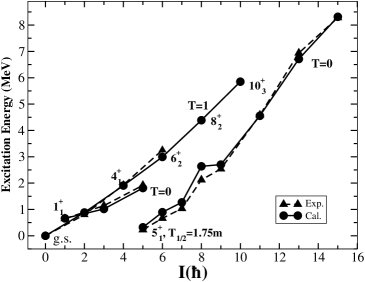
Figure 4: Calculated and experimental Oleary02 lowest $T=1$ and $T=0$ states in ⁵⁰Mn. The $T=0$ states from $5^{+}$ to $15^{+}$ forms the $K^{\pi}=5^{+}$ band.

Three negative-parity states with possible $8^{-},~{}10^{-}$ and $12^{-}$ assignments were observed in ⁵⁰Mn Svensson98 . This band has been tentatively interpreted as an octupole vibration band coupled to the $5^{+}_{1}$ isomeric state by Svensson et al. Svensson98 . In the shell model, the negative-parity band could be generated in the $sdfp$ shell with one particle exciting from the $0d_{3/2}$ orbital.

Figure 5: Proposed isovector M1 transitions between the two $K=0^{+}$ bands in ⁵⁰Mn. Calculated decay strengths (in $\mu_{N}^{2}$) are shown along with the transition arrows.

IV Electromagnetic properties

The electromagnetic (EM) transition properties of excited states can provide other detailed structure information. Particularly, EM properties play important roles in the identifications of various bands. In the following, we will investigate E2 and M1 transition properties in ⁴⁶V and ⁵⁰Mn, with a detailed analyse for ⁵⁰Mn.

In practical shell-model calculations, transitions are treated in the truncated configuration. The wave functions ($\Phi_{\lambda}$) of nuclear states are in fact the projections of the full-Hamiltonian wave functions ($\Psi_{\lambda}$) onto the model space with introducing an effective interaction as described by Eq. (3). Hence, renormalized EM transition operators should be used to include effects from the excluded space,

$$\langle\Psi_{f}|\mathcal{O}|\Psi_{i}\rangle\longrightarrow\langle\Phi_{f}|\mathcal{O}_{\text{eff}}|\Phi_{i}\rangle,$$ (14)

where $i$ and $f$ indicate the initial and final states.

Table 1: Calculated and observed B(E2) values (in e²fm⁴) in ⁵⁰Mn. Two groups of effective charges are used. One is the “standard” charges with $e_{p}$=1.50e, $e_{n}$=0.50e; the other one with $e_{p}$=1.15e, $e_{n}$=0.80e taken from Ref. duRietz04 . Experimental data are taken from Ref. Pietralla02 .

	$e_{p}$=1.50e, $e_{n}$=0.50e			$e_{p}$=1.15e, $e_{n}$=0.80e
$(J_{i},T_{i})\rightarrow(J_{f},T_{f})$	HO	WS	SKcsb	HO	WS	SKcsb	EXP
$K=5^{+}$
$(7_{1}^{+},0)\rightarrow(5_{1}^{+},0)$	45	42	37	42	39	35
$(9_{1}^{+},0)\rightarrow(7_{1}^{+},0)$	151	143	126	142	133	118	$\geq 115^{+23}_{-19}$
$(11_{1}^{+},0)\rightarrow(9_{1}^{+},0)$	159	151	133	150	141	125
$(13_{1}^{+},0)\rightarrow(11_{1}^{+},0)$	119	114	101	114	107	95
$(15_{1}^{+},0)\rightarrow(13_{1}^{+},0)$	58	55	49	55	52	46
$K=0^{+}$
$(3_{1}^{+},0)\rightarrow(1_{1}^{+},0)$	214	205	178	203	191	167	$700^{+240}_{-190}$
$(5_{2}^{+},0)\rightarrow(3_{1}^{+},0)$	189	182	158	180	170	148	$<1880$
$(7_{2}^{+},0)\rightarrow(5_{2}^{+},0)$	168	163	141	160	151	132
$(9_{2}^{+},0)\rightarrow(7_{2}^{+},0)$	85	83	71	81	77	67
$(11_{2}^{+},0)\rightarrow(9_{2}^{+},0)$	4.5	4.4	3.9	4.3	4.1	3.7

Table 2: Calculated reduced transition strengths of M1 (in $\mu^{2}_{N}$) and E2 (in e²fm⁴) transitions in ⁴⁶V. Experimental data are taken from Refs. Brandolini01 ; Brentano01 .

	B(E2)			B(M1)
$J_{i}\rightarrow J_{f}$	Cal.	Exp.		Cal.	Exp.
$K=3^{+}$
$5_{1}^{+}\rightarrow 3_{1}^{+}$	29	67(14)
$7_{1}^{+}\rightarrow 5_{1}^{+}$	2	97(15)
$9_{1}^{+}\rightarrow 7_{1}^{+}$	173	159(34)
$11_{1}^{+}\rightarrow 9_{1}^{+}$	153	139(26)
$13_{1}^{+}\rightarrow 11_{1}^{+}$	109	78(16)
$15_{1}^{+}\rightarrow 13_{1}^{+}$	78	60(12)
$4_{1}^{+}\rightarrow 3_{1}^{+}$	280	208(50)		$4\times 10^{-4}$
$6_{1}^{+}\rightarrow 5_{1}^{+}$	157			$9\times 10^{-4}$
$8_{1}^{+}\rightarrow 7_{1}^{+}$	33			$2\times 10^{-7}$
$10_{1}^{+}\rightarrow 9_{1}^{+}$	33			$3\times 10^{-5}$
$6_{1}^{+}\rightarrow 4_{1}^{+}$	96
$8_{1}^{+}\rightarrow 6_{1}^{+}$	138
$10_{1}^{+}\rightarrow 8_{1}^{+}$	130
$K=0^{+}$
$2_{1}^{+}\rightarrow 0_{1}^{+}$	176	138(35)
$4_{2}^{+}\rightarrow 2_{1}^{+}$	237	$>169$
$6_{2}^{+}\rightarrow 4_{2}^{+}$	$221$
$8_{3}^{+}\rightarrow 6_{2}^{+}$	212
$10_{2}^{+}\rightarrow 8_{3}^{+}$	161
$12_{3}^{+}\rightarrow 10_{2}^{+}$	0.03
$3_{2}^{+}\rightarrow 1_{1}^{+}$	217
$5_{2}^{+}\rightarrow 3_{2}^{+}$	117
$7_{2}^{+}\rightarrow 5_{2}^{+}$	0.07
$\Delta K=0,~{}~{}\Delta T=1$
$1_{1}^{+}\rightarrow 0_{1}^{+}$				1.49	$\geq 0.77$
$3_{2}^{+}\rightarrow 2_{1}^{+}$	0.05			1.14	2.0(7)
$4_{2}^{+}\rightarrow 3_{2}^{+}$	0.15			1.0	0.57(15)
$4_{2}^{+}\rightarrow 5_{2}^{+}$				1.26	0.55(13)
$6_{2}^{+}\rightarrow 5_{2}^{+}$	0.11			0.33
$7_{2}^{+}\rightarrow 6_{2}^{+}$	0.12			0.03
$8_{2}^{+}\rightarrow 7_{2}^{+}$	3.7			0.06
$\Delta K=3,~{}~{}\Delta T=1$
$2_{1}^{+}\rightarrow 3_{1}^{+}$	0.4			0.26
$3_{2}^{+}\rightarrow 3_{1}^{+}$	2.9			2$\times 10^{-5}$
$4_{2}^{+}\rightarrow 3_{1}^{+}$				0.04	0.012
$4_{2}^{+}\rightarrow 5_{1}^{+}$				0.236	0.02
$5_{2}^{+}\rightarrow 3_{1}^{+}$	57

With the folded-diagram method, effective model-dependent transition operators can de derived microscopically Siiskonen01 ; Engeland00 . However, a simple way to evaluate the renormalization effect is to introduce the effective charges of nucleons Brown01 . For example, the effective operator for E2 transitions can be given as,

$$\mathcal{O}(\text{el}.,2M)=\sum_{i}(\tilde{e}_{\tau}/e)r_{i}^{2}Y_{2}^{M}(\theta_{i},\phi_{i}),$$ (15)

where $i$ sums over all particles and $\tilde{e}_{\tau}$ (with $\tau=\mu,~{}\nu$) are renormalized effective charges for protons and neutrons, respectively.

Table 1 gives the shell-model predictions of B(E2) values for $K^{\pi}=5^{+}$ and $K^{\pi}=0^{+}$ bands ($T=0$) in ⁵⁰Mn. Two different groups of empirical effective charges have been used. One is the commonly-used effective charges of $e_{p}=1.5e$ and $e_{n}=0.5e$. The other group with $e_{p}=1.15e$ and $e_{n}=0.80e$ was extracted from the B(E2; $27/2^{-}\rightarrow 23/2^{-}$) values of $T=1/2$ mirror nuclei ⁵¹Fe and ⁵¹Mn by du Rietz et al. duRietz04 . The wave functions of the shell model are calculated with three different bases, i.e., the harmonic oscillator (HO), the Woods-Saxon (WS) potential and the Skyrme force (SKcsb) by Brown et al. Brown00 in which a charge-symmetry-breaking term has been added. In the $K=5^{+}$ band ($T=0$) of ⁵⁰Mn, one E2 strength has been determined Pietralla02 . The calculated B(E2, $9_{1}^{+}\rightarrow 7^{+}_{1}$) value agrees with the measured lower limit. As seen from Table 1, calculated decay strengths are relatively stable for different choices of effective charges and single-particle wave functions. Reduced E2 decay strengths for ⁴⁶V are shown in Table 2 in which the results calculated with the HO single-particle wave function and effective charges of e_p=1.5e and e_n=0.5e are given.

Figure 6: Decay scheme and B(E2) strengths (in e²fm⁴) of the proposed T=1 band in ⁵⁰Mn. Calculated and experimental strengths Pietralla02 are shown on the right- and left-hand sides of the transition lines, respectively.

Fig. 6 shows the calculations of electrical quadruple transitions for the $T=1$ band in ⁵⁰Mn. Results were calculated with $e_{p}=1.5e$ and $e_{n}=0.5e$ and HO single-particle wave functions. Three side bands identified experimentally are shown in the figure. Two bands with $T=0$ on the right side of the figure have been assigned with $K^{\pi}=3^{+}$ and $K^{\pi}=2^{+}$, respectively, by Sahu et al. Sahu03 . The proposed $10^{+}_{1}$ state ($T=0$) at 5027 keV, and the $8^{+}_{2}$ state ($T=1$) at 4386 keV have not been observed. Calculated $8^{+}_{3}$ and $10^{+}_{2}$ states are recognized as the observed $8^{+}$ state at 4874 keV and the $10^{+}$ state at 6460 keV, respectively. Both states have the isospin of $T=0$ since M1 transition strengths are rather weak compared with inner-band E2 transitions.

The magnetic dipole (M1) operator is dominated by the isovector spin ($\sigma$) term. Strong M1 transitions have been observed only in light nuclei. In the fp shell, due to the coexistence of $T=0$ and $T=1$ bands at low excitation energies, strong isovector ($\Delta T=1$) M1 transitions have been expected Oleary02 ; Pietralla02 . We take the g-factor values of free nucleon and the HO basis to investigate the isoscalar and isovector M1 transition properties in ⁴⁶V and ⁵⁰Mn.

Table 3: Calculated reduced matrix elements (in $\mu^{2}_{N}$) for M1 transitions in ⁵⁰Mn with the g-factors of free nucleon [g_s(proton)=5.586, g_s(neutron)=-3.826, g_l(proton)=1 and g_l(neutron)=0]. Experimental data are taken from Ref. Pietralla02 . Calculated B(E2) values are also shown.

	B(E2)	B(M1)
$(J_{i},T_{i})\rightarrow(J_{f},T_{f})$	Cal.	Cal.	Exp.
$\Delta T=1$
$(1_{1}^{+},0)\rightarrow(0_{1}^{+},1)$		2.70
$(2_{1}^{+},1)\rightarrow(1_{1}^{+},0)$	0.28	2.27	$<$6.7
$(3_{1}^{+},0)\rightarrow(2_{1}^{+},1)$	0.78$\times 10^{-2}$	2.94	$2.9^{+10}_{-7}$
$(4_{1}^{+},1)\rightarrow(3_{1}^{+},0)$	0.70	3.13	$1.05^{+31}_{-20}$
$(6_{2}^{+},1)\rightarrow(5_{2}^{+},0)$	1.46	1.98	$>$0.24
$(7_{2}^{+},0)\rightarrow(6_{2}^{+},1)$	0.30	0.93
$(8_{2}^{+},1)\rightarrow(7_{2}^{+},0)$	1.66	1.31
$(9_{2}^{+},0)\rightarrow(8_{2}^{+},1)$	0.93$\times 10^{-2}$	0.48
$(10_{3}^{+},1)\rightarrow(9_{2}^{+},0)$	0.43	0.31
$(11_{2}^{+},0)\rightarrow(10_{3}^{+},1)$	3.76	0.04
$\Delta T=0$
$(4_{2}^{+},0)\rightarrow(3_{1}^{+},0)$	2.0	8.65$\times 10^{-5}$
$(4_{3}^{+},0)\rightarrow(3_{1}^{+},0)$	0.34	4.67$\times 10^{-2}$
$(8_{3}^{+},0)\rightarrow(7_{2}^{+},0)$	7.5	$4.30\times 10^{-4}$
$(10_{2}^{+},0)\rightarrow(9_{2}^{+},0)$	0.08	0.023
$(11_{2}^{+},0)\rightarrow(10_{2}^{+},0)$	35	0.06

Part of calculated M1 transition strengths for ⁴⁶V and ⁵⁰Mn are shown in Table 2 and 3, respectively. Available experimental data are given for comparison. Our calculations clearly show that $\Delta T=1$, M1 transitions with $\Delta K=0$ are enhanced, while other $\Delta T=1$, M1 transitions are retarded due to the K quantum number selection (M1 transitions with $\Delta K\geq 1$ should be highly hindered). In ⁴⁶V, four strong isovector M1 transitions have been observed. They were reproduced well in our calculations. In ⁵⁰Mn, the uncertainty in experimental data is very large Pietralla02 . Calculated $\Delta K=0$ inter-band M1 transitions ($\Delta T=1$) are shown in Fig. 5. The strong M1 transitions have also been interpreted by a simple picture of quasideuteron configurations of odd neutron and odd proton in ⁵⁰Mn Pietralla02 .

Another exciting problem involving odd-odd $N=Z$ nuclei is the study of super-allowed decays. The $ft$ values of ground-state Fermi ($0^{+}\rightarrow 0^{+}$) decays would be the same for analogous transitions if the conserved vector current (CVC) hypothesis is valid Hardy05 . Odd-odd $N=Z$ nuclei provide the best ground to test the understanding of the electroweak interaction. As discussed in Ref. Hardy05 , the isospin-symmetry breaking effect has significant contribution on the asymmetry in analogous transitions. In our Hamiltonian, the isospin symmetry breaking is treated microscopically, which can provide a basis to quantify the effect. However, it is beyond the scope of this paper.

V Conclusion

A microscopical fp-shell interaction has been constructed from the high-precision CD Bonn NN potential using the folded-diagram renormalization method. In the CD Bonn potential, both charge symmetry breaking and charge independence breaking are well described. The Coulomb field is also included in calculating the effective interaction. Hence, in our effective Hamiltonian, isospin symmetry is naturally broken. The isospin-nonconserving interaction has been used to investigate the level structures of odd-odd self-conjugate nuclei in the lower part of fp shell. Excellent agreements between calculations and experiments have been obtained. Particularly, the interaction gave a good description of the isospin structures in odd-odd $N=Z$ nuclei, reproducing well the relative positions of $T=0$ and $T=1$ bands. Further studies done with the Idaho-A chiral perturbation potential showed similar results. Moreover, calculations show that effective interactions derived with the folded-diagram method can reproduce the low-lying structures of odd-odd $N=Z$ nuclei in other major shells, including the famous case of ${}^{10}_{~{}5}$B in p shell. Our calculations reproduce the high-spin isomeric states in the fp shell. In particular, we have performed detailed shell-model calculations for the positive-parity states in ⁴⁶V and ⁵⁰Mn. EM transition properties and isospin structures in odd-odd $N=Z$ nuclei have been predicted and discussed. We can construct a one-to-one correspondence between calculated results and experimental data with the comparisons of excitation energies and electromagnetic transition properties. Our study shows that the predictions of this ab initio interaction is encouraging. It is very interesting to test its performance in other fp shell nuclei. Further studies will be carried out in our future works.

References

- (1) D.J. Dean and M. Hjorth-Jensen, Rev. Mod. Phys. 75, 607 (2003).
- (2) A.O. Macchiavelli, et al., Phys. Rev. C 61, 041303(R) (2000).
- (3) W. Satuła and R. Wyss, Phys. Lett B393, 1 (1997); Phys. Rev. Lett 86, 4488 (2001).
- (4) J. Jänecke and T.W. O’Donnell, Phys. Lett. B605, 87 (2005), and reference therein.
- (5) P. Vogel, Nucl. Phys. A 662, 148 (2000).
- (6) I. Schneider, et al., Phys. Rev. C 61, 044312 (2000).
- (7) C. Frießner, et al., Phys. Rev. C 60, 011304 (1999).
- (8) A. Schmidt, et al., Phys. Rev. C 62, 044319 (2000).
- (9) C.E. Svensson, et al., Phys. Rev. C 58, R2621 (1998).
- (10) C.D. O’Leary, et al.,, Phys. Lett. B525, 49 (2002).
- (11) C.D. O’Leary, et al., Phys. Lett. B459, 73 (1999).
- (12) N. Pietralla et al., Phys. Rev. C 65, 024317 (2002).
- (13) S. Skoda, et al., Phys. Rev. C 58, R5 (1998).
- (14) S.M. Lenzi, et al., Phys. Rev. C 60, 021303 (1999).
- (15) A. Petrovici, K.W. Schmid, and A. Faessler, Nucl. Phys. A647, 197 (1999).
- (16) A. Poves and G. Martínez-Pinedo, Phys. Lett. B430, 203 (1998).
- (17) F. Brandolini et al., Phys. Rev. C 64, 044307 (2001).
- (18) P. von Brentano et al., Nucl. Phys. A682, 48c (2001).
- (19) S.M. Lenzi et al., Phys. Rev. Lett. 87, 122501 (2001).
- (20) P.E. Garrett et al., Phys. Rev. Lett. 87, 132502 (2001).
- (21) A.P. Zuker, S.M. Lenzi, G. Martínez-Pinedo, and A. Poves, Phys. Rev. Lett. 89, 142502 (2002).
- (22) R. Machleidt, Phys. Rev. C 63, 024001 (2001).
- (23) T.T.S. Kuo and E. Osnes, Folded-Diagram Theory of Effective Interaction in Nuclei, Atoms and Molecules, Springer Lecture Notes in Physics, Vol. 364 (Springer-Verlag, Berlin, 1990).
- (24) S. Cohen and D. Kurath, Nucl. Phys. 73, 1 (1965).
- (25) B.H. Wildenthal, Prog. Part. Nucl. Phys. 11, 5 (1984).
- (26) T.T.S. Kuo and G.E. Brown, Nucl. Phys. A114, 241 (1968).
- (27) A. Poves and A. Zuker, Phys. Rep. 70, 235 (1981).
- (28) E. Caurier, G. Martínez-Pinedo, F. Nowacki, A. Poves, and A.P. Zuker, Rev. Mod. Phys. 77, 427 (2005).
- (29) W.A. Richter, M.G. van der Merwe, R.E. Julies, and B.A. Brown, Nucl. Phys. A704, 134 (1991).
- (30) M. Honma, T. Otsuka, B.A. Brown, and T. Mizusaki, Phys. Rev. C 65, 061301(R) (2002).
- (31) E. Caurier, A.P. Zuker, A. Poves, and G. Martínez-Pinedo, Phys. Rev. C 50, 225 (1994).
- (32) E. Caurier et al., Phys. Rev. Lett. 75, 2466 (1995).
- (33) G. Martínez-Pinedo, A.P. Zuker, A. Poves, and E. Caurier, Phys. Rev. C 55, 187 (1996).
- (34) S.K. Bogner, T.T.S. Kuo, and A. Schwenk, Phys. Rep. 386, 1 (2003).
- (35) H. Feldmeier, T. Neff, R. Roth, and J. Schnack, Nucl. Phys. A 632, 61 (1998).
- (36) M. Hjorth-Jensen, T.T.S. Kuo, and E. Osnes, Phys. Rep. 261, 125 (1995).
- (37) D.R. Entem and R. Machleidt, Phys. Lett. B524, 93 (2002).
- (38) Table of Isotopes, 8th ed., edited by R.B. Firestone and V.S. Shirley (Wiley, New York, 1996) Vol. 2.
- (39) A. Etchegoyen, W.D.M. Rae, N.S. Godwin, W.A. Richter, C.H. Zimmerman, B.A. Brown, W.E. Ormand, and J.S. Winfield, MSU-NSCL Report No. 524 (1985).
- (40) B.A. Brown, Prog. Part. Nucl. Phys. 47, 517 (2001).
- (41) T. Siiskonen, M. Hjorth-Jensen, and J. Suhonen, Phys. Rev. C 63, 055501 (2001).
- (42) T. Engeland, M. Hjorth-Jensen, and E. Osnes, Phys. Rev. C 61, 021302 (2000).
- (43) R. du Rietz et al., Phys. Rev. Lett. 93, 222501 (2004).
- (44) B.A. Brown, W.A. Richter, and R. Lindsay, Phys. Lett. B483, 49 (2000).
- (45) R. Sahu and V.K.B Kota, Phys. Rev. C 67, 054323 (2003).
- (46) J.C. Hardy and I.S. Towner, Phys. Rev. C 71, 055501 (2005).