Three-body model calculations for ¹⁶C nucleus

Abstract

We apply a three-body model consisting of two valence neutrons and the core nucleus ¹⁴C in order to investigate the ground state properties and the electronic quadrupole transition of the ¹⁶C nucleus. The discretized continuum spectrum within a large box is taken into account by using a single-particle basis obtained from a Woods-Saxon potential. The calculated B(E2) value from the first 2⁺ state to the ground state shows good agreement with the observed data with the core polarization charge which reproduces the experimental B(E2) value for ¹⁵C. We also show that the present calculation well accounts for the longitudinal momentum distribution of ¹⁵C fragment from the breakup of ¹⁶C nucleus. We point out that the dominant ($d_{5/2})^{2}$ configuration in the ground state of ¹⁶C plays a crucial role for these agreement.

Nuclei far from the $\beta$ stability line often reveal unique phenomena originating from a large asymmetry in the neutron and proton numbers. One of the typical examples is a neutron collective mode, which is characterized only by the neutron excitation, with negligible contribution from the proton excitation. A recent calculation based on the continuum quasi-particle random phase approximation (QRPA) has, in fact, predicted the existence of such neutron mode in the low-lying quadrupole excitation in ²⁴O M01 .

Recently, the electric quadrupole (E2) transition from the first 2⁺ state at 1.766 MeV to the ground state in ¹⁶C has been measured at RIKEN IOA04 . The observed B(E2) value (0.26$\pm$0.05 Weisskopf units) has turned out to be surprisingly small, as compared to the known systematics in stable nuclei. On the other hand, a distorted wave Born approximation (DWBA) analysis for the ¹⁶C + ²⁰⁸Pb inelastic scattering indicates a large enhancement of the ratio of the neutron to proton transition amplitudes, $M_{n}/M_{p}$=7.6$\pm$1.7 EDK04 , that is considerably larger than the isoscalar value, $N/Z$=1.67. A similar value for $M_{n}/M_{p}$ was also obtained from the inelastic proton scattering from the ¹⁶C nucleus OIA06 . These experimental data suggest that the first 2⁺ state in ¹⁶C is a good candidate for the neutron excitation mode.

There have already been various theoretical calculations for the structure of ¹⁶C nucleus KE05 ; SZZT04 ; TIOI04 ; SMA04 ; HY06 ; FMOSA06 . Except for a recent microscopic shell-model calculation FMOSA06 , however, they all fail to reproduce the anomalously hindered E2 transition. For instance, Suzuki and his collaborators have solved a $n+n+^{14}$C three-body model and found that the E2 strength is overestimated by a factor of about 2 if the same core polarization charge is employed as that used to describe the ¹⁵C nucleus. A similar overestimation of B(E2) value was found also in the antisymmetrized molecular dynamics (AMD) calculation KE05 as well as in the deformed Skyrme Hartree-Fock calculation SZZT04 .

In this paper, we apply a three-body model with a finite-range $n$-$n$ interaction SMA04 ; HY06 to describe the ground and excited states in the ¹⁶C nucleus. We employ the single-particle (s.p.) basis obtained from a $n$-¹⁴C Woods-Saxon potential to diagonalize the three-body Hamiltonian. The continuum s.p. spectrum is discretized in a large box. Notice that the effect of continuum couplings can be properly accounted for with such s.p. basis cd . A similar three-body model with a density-dependent contact interaction has successfully been applied to describe the structure of Borromean nuclei BE91 ; EBH99 ; VMP96 ; HS05 ; HSCS06 . In Refs. SMA04 ; HY06 , Suzuki et al. adopted the correlated Gaussian basis to diagonalize a similar three-body Hamiltonian for ¹⁶C. However, it remains an open question whether the correlated Gaussian basis is efficient enough to take into account the continuum couplings. Therefore, our study can be considered as a complement to the previous studies in Refs.SMA04 ; HY06 .

Assuming that the effect of core excitation on the low-lying spectrum of the ¹⁶C nucleus is negligible SMA04 ; VM95 , we consider the following three-body Hamiltonian:

$$H=\hat{h}(1)+\hat{h}(2)+V_{nn}+\frac{\mbox{\boldmath$p$}_{1}\cdot\mbox{\boldmath$p$}_{2}}{A_{c}m},$$ (1)

where $m$ and $A_{c}$ are the nucleon mass and the mass number of the inert core nucleus, respectively. $\hat{h}$ is the s.p. Hamiltonian for a valence neutron interacting with the core. The diagonal component of the recoil kinetic energy of the core nucleus is included in $\hat{h}$, whereas the off-diagonal part is taken into account in the last term in the Hamiltonian (1). We use a Woods-Saxon potential for the interaction in $\hat{h}$,

$$V_{nC}(r)=\left(V_{0}+V_{ls}\,(\mbox{\boldmath$l$}\cdot\mbox{\boldmath$s$})\frac{1}{r}\frac{d}{dr}\right)\left[1+\exp\left(\frac{r-R}{a}\right)\right]^{-1},$$ (2)

where $R=r_{0}A_{c}^{1/3}$. The parameter sets for the Woods-Saxon potential which we employ in this paper are listed in Table I. The sets A, B, and C were used in Ref. SMA04 ; HY06 , while the set D was used in Ref. VM95 in order to discuss the role of particle-vibration coupling in the ¹⁵C nucleus. These parameter sets yield almost the same value for the energy of the 2$s_{1/2}$ state, $\epsilon_{2s_{1/2}}\sim-1.21$ MeV, and of the the 1$d_{5/2}$ state, $\epsilon_{1d_{5/2}}\sim-0.47$ MeV.

Table 1: Parameters for the Woods-Saxon neutron-core potential, $V_{nC}$, in Eq. (2).

Set	$V_{0}$ (MeV)	$V_{ls}$ (MeV fm2)	$r_{0}$ (fm)	$a$ (fm)
A	$-$50.31	16.64	1.25	0.65
B	$-$50.31 ($l$=0)	31.25	1.25	0.65
	$-$47.18 ($l\neq 0$)
C	$-$51.71	26.24	1.20	0.73
D	$-$44.41	31.52	1.27	0.90

In our previous works HS05 ; HSCS06 , we used the density-dependent delta force BE91 ; EBH99 for the interaction between the valence neutrons, $V_{nn}$. However, we here use the same finite-range force as in Ref. SMA04 in order to compare our results with those of Refs. SMA04 ; HY06 . That is the singlet-even part of the Minnesota potential Minnesota ,

$$V_{nn}(\mbox{\boldmath$r$}_{1},\mbox{\boldmath$r$}_{2})=v_{0}\,e^{-b_{0}(\mbox{\boldmath$r$}_{1}-\mbox{\boldmath$r$}_{2})^{2}}+v_{1}\,e^{-b_{1}(\mbox{\boldmath$r$}_{1}-\mbox{\boldmath$r$}_{2})^{2}},$$ (3)

with $v_{0}$=200 MeV, $b_{0}$=1.487 fm^-2, and $b_{1}$=0.465 fm^-2. Following Ref. SMA04 , we adjust the value of $v_{1}$ for each parameter set of the Woods-Saxon potential so that the ground state energy of ¹⁶C, $E_{\rm gs}=-5.47$ MeV, is reproduced.

Table 2: Properties of the ground and the second 0⁺ states obtained with several parameter sets for the neutron-core potential, $V_{nC}$. $P_{ss}$ and $P_{dd}$ are the probability for the $[(2s_{1/2})^{2}]$ and $[(1d_{5/2})^{2}]$ components in the wave function, respectively. $P_{S=0}$ is the probability of the spin-singlet ($S=0$) component in the ground state. $E_{0^{+}_{2}}$ is the excitation energy for the second 0⁺ state in the unit of MeV, while $r(^{16}$C) is the root-mean-square radius of the ¹⁶C nucleus in the unit of fm. The experimental values are $E_{0^{+}_{2}}({\rm exp})=$3.00 MeV and $r(^{16}$C; exp)=2.64 $\pm$ 0.05 fm Z02 , respectively.

Set	$P_{ss}$(g.s.)	$P_{dd}$(g.s.)	$P_{S=0}$	$r(^{16}$C)	$E_{0^{+}_{2}}$	$P_{ss}$(0${}_{2}^{+}$)	$P_{dd}(0_{2}^{+})$
A	0.184	0.699	0.784	2.56	2.32	0.755	0.201
B	0.177	0.711	0.746	2.56	2.35	0.775	0.187
C	0.183	0.696	0.768	2.57	2.39	0.763	0.196
D	0.206	0.633	0.808	2.64	2.48	0.733	0.221

The three-body Hamiltonian (1) is diagonalized by expanding the two-particle wave function $\Psi(\mbox{\boldmath$r$}_{1},\mbox{\boldmath$r$}_{2})$ with the eigenfunction $\phi_{nljm}$ of the s.p. Hamiltonian $\hat{h}$, where $n$ is the radial quantum number. The continuum s.p. states are discretized with a box size of $R_{\rm box}=30$ fm. We include the s.p. angular momentum $l_{1}$ and $l_{2}$ up to 5, and truncate the model space of the two-particle states at $\epsilon_{1}+\epsilon_{2}$ = 30 MeV, where $\epsilon$ is the s.p. energy of the valence particle. We have checked that the results do not significantly change even if we truncate the model space at 60 or 80 MeV, as long as $v_{1}$ in Eq. (3) is adjusted for each model space. In the diagonalization, we explicitly exclude the $1s_{1/2},1p_{3/2}$, and $1p_{1/2}$ states, which are occupied by the core nucleus. The results for the ground state and the second 0⁺ state are summarized in Table II. The parameter set dependence is small, although the set D reproduces the excitation energy of the second 0⁺ state, $E_{0_{2}^{+}}$, and the root-mean-square (rms) radius of the ¹⁶C nucleus, $r(^{16}$C), slightly better than the other parameter sets. The latter quantity is calculated as BE91 ; EBH99 ; VMP96

$$\langle r^{2}\rangle_{A_{c}+2}=\frac{A_{c}}{A_{c}+2}\langle r^{2}\rangle_{A_{c}}+\frac{1}{A_{c}+2}\,\left(\frac{2A_{c}\,\langle\rho^{2}\rangle}{A_{c}+2}+\frac{\langle\lambda^{2}\rangle}{2}\right),$$ (4)

where $\mbox{\boldmath$\lambda$}=(\mbox{\boldmath$r$}_{1}+\mbox{\boldmath$r$}_{2})/2$ and $\mbox{\boldmath$\rho$}=\mbox{\boldmath$r$}_{1}-\mbox{\boldmath$r$}_{2}$. Following Refs. SMA04 ; HY06 , we take 2.35 fm for the rms radius of the core nucleus, $\sqrt{\langle r^{2}\rangle_{A_{c}}}$. We find that the rms radius of ¹⁶C is well reproduced in the present calculations.

We notice that our results are considerably different from those of Refs. SMA04 ; HY06 concerning the probability for the $[(2s_{1/2})^{2}]$ and $[(1d_{5/2})^{2}]$ components in the wave function, which are denoted by $P_{ss}$ and $P_{dd}$ in Table II, respectively. Our results show that the ground state of ¹⁶C mainly consists of the $[(1d_{5/2})^{2}]$ configuration, while the second 0⁺ state is dominated by the $[(2s_{1/2})^{2}]$ configuration. This is in contrast to the results of Refs. SMA04 ; HY06 , which show the dominance of the $[(2s_{1/2})^{2}]$ component in the ground state. As a consequence, we also obtain a smaller value of the spin-singlet probability, $P_{S=0}$, than in Ref. HY06 . Notice that the d-wave dominance was suggested from the analyses of longitudinal momentum distribution for the one-neutron knockout reaction of ¹⁶C MAB01 ; Y03 . We will discuss the longitudinal momentum distribution later in this paper.

It is worthwhile to consider a simple two-level pairing model consisting of the 2$s_{1/2}$ and 1$d_{5/2}$ s.p. levels in order to illustrate how the $[(1d_{5/2})^{2}]$ configuration becomes dominant in the ground state of ¹⁶C. If there were no interaction between the valence neutrons, the ground state wave function would be the pure $[(2s_{1/2})^{2}]$ state, since the s.p. energy for the 2$s_{1/2}$ state is lower than that for the 1$d_{5/2}$ state ($\epsilon_{2s_{1/2}}=-1.21$ MeV and $\epsilon_{1d_{5/2}}=-0.47$ MeV) . If one assumes a delta interaction, $V_{nn}=-g\,\delta(\mbox{\boldmath$r$}_{1}-\mbox{\boldmath$r$}_{2})$ between the valence neutrons, the diagonal matrix element of the Hamiltonian reads BB05

$$H_{ii}=2\epsilon_{i}-g\,\frac{2j+1}{8\pi}\,I_{ii},$$ (5)

where $I_{ii}$ is the radial integral for the configuration $(i)^{2}$. Therefore, the pairing interaction influences the $[(1d_{5/2})^{2}]$ configuration more strongly than the $[(2s_{1/2})^{2}]$ configuration by a factor of 3 when the radial integral $I_{ii}$ is similar to each other. If we choose the strength $g$ so that the ground state energy is reproduced within the two-level model, we find $g$=1005 MeV$\cdot$fm^-3 for the parameter set D. This leads to the diagonal matrix element of $H_{ii}=-3.70$ MeV for $i=2s_{1/2}$ and $H_{ii}=-4.85$ MeV for $i=1d_{5/2}$, lowering the $[(1d_{5/2})^{2}]$ configuration in energy. Taking into account the off-diagonal matrix element and diagonalizing the 2$\times$2 matrix, we find $P_{ss}$=0.26 and $P_{dd}$=0.74 for the ground state, which are very close to the results shown in Table II.

The upper panels of Figs. 1 and 2 show the two-particle densities $\rho_{2}(r_{1},r_{2},\theta)$ for the ground state and the second 0⁺ state, respectively. These are obtained with the Minnesota potential and the parameter set D for the s.p. potential. In order to facilitate the presentation, we set $r_{1}=r_{2}=r$ and multiply the weight factor of $8\pi^{2}r^{4}\sin\theta$ HS05 . Despite that $P_{ss}$ and $P_{dd}$ are considerably different, we obtain similar density distributions to those in Ref. HY06 . In particular, we observe similar “di-neutron” and “cigar-like” configurations in the ground state, as well as “boomerang” configuration HY06 in the second 0⁺ state as in Ref. HY06 . The lower panels of Figs. 1 and 2 show the angular densities $\rho(\theta)$ obtained by integrating the radial coordinates in the two-particle density HS05 . It is multiplied by a weight factor of 2$\pi\sin\theta$. As a comparison, we also show the angular densities for the pure $[(2s_{1/2})^{2}]$ and $[(1d_{5/2})^{2}]$ configurations by the dotted and dashed lines, respectively. They are given by $\rho(\theta)=1/4\pi$ for the $[(2s_{1/2})^{2}]$ configuration and $\rho(\theta)=3/4\pi\cdot(5/4\cdot\cos^{4}\theta+3/20)$ for the $[(1d_{5/2})^{2}]$ configuration. As we see in the figures, the angular density for the ground state is close to that for the pure $[(1d_{5/2})^{2}]$ configuration, while the angular density for the second 0⁺ state is close to that for the pure $[(2s_{1/2})^{2}]$ configuration, being consistent with the calculated values for $P_{dd}$ and $P_{ss}$ listed in Table II.

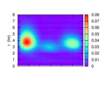
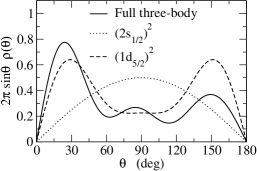
Figure 1: (Color online) (the upper panel) The two-particle density for the ground state of ¹⁶C obtained with the parameter set D for the single-particle potential as a function of $r_{1}=r_{2}=r$ and the angle between the valence neutrons, $\theta$. It is weighted with a factor of $8\pi^{2}r^{4}\sin\theta$. (the lower panel) The corresponding angular density weighted with a factor 2$\pi\sin\theta$. The solid line is the result of the three-body model calculation with the Minnesota potential. The dotted and the dashed lines are for the pure $[(2s_{1/2})^{2}]$ and $[(1d_{5/2})^{2}]$ configurations, respectively.

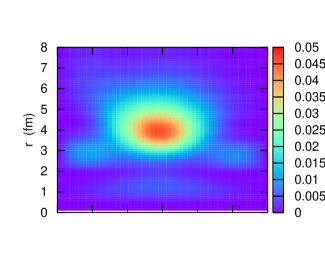
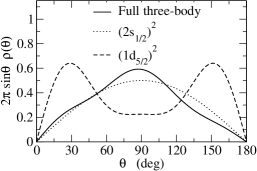
Figure 2: (Color online) Same as Fig. 1, but for the second 0⁺ state of ¹⁶C.

We next discuss the quadrupole excitation in ¹⁶C. Table III summarizes the results of the present three-body model for the first 2⁺ state. The energy of the 2⁺ state is well reproduced with this model, especially with the parameter set D. As compared to the results of Refs. SMA04 ; HY06 , the probabilities for the $[2s_{1/2}1d_{5/2}]$ and $[(1d_{5/2})^{2}]$ components, denoted as $P_{sd}$ and $P_{dd}$, respectively, are comparable to each other in our calculation, whereas $P_{sd}$ is much larger than $P_{dd}$ in Ref. HY06 .

Table 3: Properties of the first 2⁺ state of ¹⁶C obtained with several parameter sets for the neutron-core potential, $V_{nC}$. $P_{sd}$ and $P_{dd}$ are the probability for the $[(2s_{1/2})\times(1d_{5/2})]$ and $[(1d_{5/2})^{2}]$ components in the wave function, respectively. $E_{2^{+}}$ is the excitation energy in the unit of MeV, while B(E2) is the electric quadrupole transition strength from the 2⁺ state to the ground state, in the unit of $e^{2}$fm⁴. The experimental values are $E_{2^{+}}$ (exp)=1.77 MeV and B(E2; exp)= 0.63 $\pm$ 0.27 $e^{2}$fm⁴ IOA04 , respectively. $e_{\rm pol}^{\rm I}$ is the core polarization charge which reproduces the experimental B(E2) value for the ¹⁵C nucleus within the $n$-¹⁴C model, whereas $e_{\rm pol}^{\rm II}$ takes into account the mass number dependence according to Eq. (11).

Set	$E_{2^{+}}$	$P_{sd}$	$P_{dd}$	$e_{\rm pol}^{\rm I}$	B(E2; $e_{\rm pol}^{\rm I}$)	$e_{\rm pol}^{\rm II}$	B(E2; $e_{\rm pol}^{\rm II}$)
A	1.26	0.392	0.504	0.162	0.972	0.145	0.808
B	1.33	0.400	0.515	0.160	0.937	0.144	0.781
C	1.34	0.402	0.500	0.153	0.956	0.137	0.797
D	1.63	0.472	0.406	0.122	1.074	0.109	0.899

In order to calculate the E2 transition strength, we introduce the core polarization charge, $e_{\rm pol}$. The E2 operator $\hat{Q}_{2\mu}$ in the present three-body model then reads (for $\mu$=0) SMA04 ; HY06 ,

$$\hat{Q}_{20}=\left(\frac{Z_{c}}{A^{2}}\,e+\frac{A^{2}-2A+2}{A^{2}}\,e_{\rm pol}\right)\sum_{i=1}^{2}r_{i}^{2}Y_{20}(\hat{\mbox{\boldmath$r$}}_{i})$$

$$+\sqrt{\frac{5}{4\pi}}\left(\frac{Z_{c}}{A^{2}}\,e-2\frac{A-1}{A^{2}}\,e_{\rm pol}\right)(2z_{1}z_{2}-x_{1}x_{2}-y_{1}y_{2}),$$ (6)

where $A=A_{c}+2$. The value of the core polarization charge which is required to fit the experimental B(E2) value in the ¹⁵C nucleus, $B(E2;5/2^{+}\to 1/2^{+})$ = 0.97 $\pm$ 0.02 $e^{2}$ fm⁴ AS91 , is listed as $e_{\rm pol}^{\rm I}$ in the fifth column in Table III. Notice that these are significantly smaller than that obtained with the harmonic vibration model of Bohr and Mottelson, $e_{\rm BM}=0.55$ for ¹⁶C, which, however, does not include the effect of loosely-bound wave functions (see Eq. (6-386b) in Ref. BM75 ). For a loosely-bound state, the polarization charge may be modified as

$$e_{\rm pol}=e_{\rm BM}\,\frac{3R^{2}/5}{\langle l_{2}j_{2}|r^{2}|l_{1}j_{1}\rangle},$$ (7)

where $R=1.2A^{1/3}$ fm and $\langle l_{2}j_{2}|r^{2}|l_{1}j_{1}\rangle$ is the radial matrix element between the s.p. states ($l_{1}j_{1}$) and ($l_{2}j_{2}$) (See Eq. (6-387) in Ref. BM75 ). With the set D, we obtain the ratio $\frac{3R^{2}}{5}/\langle 1d_{5/2}|r^{2}|2s_{1/2}\rangle$=0.205 as a reduction factor for the polarization charge for the transition from 1$d_{5/2}$ to 2$s_{1/2}$ s.p. states. This leads to $e_{\rm pol}$=0.113, which is consistent with $e_{\rm pol}^{\rm I}$ shown in Table I. A similar small value of polarization charge has been obtained also with the self-consistent Hartree-Fock (HF) + particle-vibration model SA01 . The calculated B(E2) value for ¹⁶C with $e_{\rm pol}^{\rm I}$ is listed in the sixth column in Table III. In contrast to the previous calculations with the three-body model SMA04 ; HY06 , which overestimated the B(E2) value for ¹⁶C with $e_{\rm pol}^{\rm I}$, our calculations reproduce well the experimental B(E2) value. We notice that the small value of $P_{ss}$ and $P_{sd}$ in our wave functions is responsible for good agreement with the experimental B(E2) value. For the parameter set D, the E2 matrix elements between various two-particle configurations are estimated to be,

$$\langle 2s_{1/2}\,1d_{5/2}|\hat{Q}_{20}|(2s_{1/2})^{2}\rangle=-1.087~{}~{}e\,{\rm fm^{2}},$$ (8)

$$\langle 2s_{1/2}\,1d_{5/2}|\hat{Q}_{20}|[(1d_{5/2})^{2}]^{J=0}\rangle=-0.627~{}~{}e\,{\rm fm^{2}},$$ (9)

$$\langle[(1d_{5/2})^{2}]^{J=2}|\hat{Q}_{20}|[(1d_{5/2})^{2}]^{J=0}\rangle=-0.811e\,{\rm fm^{2}}.$$ (10)

Thus, the largest matrix element is the one between the (2$s_{1/2})^{2}$ configuration in the ground state and the [2$s_{1/2}$ 1$d_{5/2}$] configuration in the 2⁺ state, although the other two matrix elements have substantial contributions. Naturally, a small value of $P_{ss}$ and $P_{sd}$ leads to a small B(E2) value, which is desired in order to reproduce the experimental data. A further improvement of the calculated value of B(E2) can be achieved if the mass number dependence of polarization charge is taken into account. In Ref. SSH03 , the result of the HF+particle-vibration model for the core polarization charge of carbon isotopes was parameterized as,

$$e_{\rm pol}=0.82\frac{Z}{A}-0.25\frac{N-Z}{A}+\left(0.12-0.36\frac{Z}{A}\,\frac{N-Z}{A}\right)\tau_{z}.$$ (11)

This formula leads to the ratio of $e_{\rm pol}$ for ¹⁶C to that for ¹⁵C to be $e_{\rm pol}(^{16}$C$)/e_{\rm pol}(^{15}$C) =0.897. The polarization charge which is scaled by this factor from $e_{\rm pol}^{\rm I}$ is denoted by $e_{\rm pol}^{\rm II}$ in Table III. We find that the calculated B(E2) values with $e_{\rm pol}^{\rm II}$ agree remarkably well with the experimental value within the experimental uncertainty.

We now discuss the longitudinal momentum distribution of ¹⁵C fragment in the breakup reaction of ¹⁶C nucleus. For this purpose, we calculate the the stripping cross section in the eikonal approximation HM85 ; HBE96 ; E96 ; BH04 . That is SMA04 ; E96 ; BH04 ,

$$\frac{d\sigma_{-n}}{dp_{z}}=\frac{1}{2\pi\hbar}\frac{1}{2l+1}\sum_{m}\int^{\infty}_{0}d^{2}b_{n}\,[1-|S_{n}(b_{n})|^{2}]$$

$$\times\int^{\infty}_{0}d^{2}r_{\perp}|S_{c}(b_{c})|^{2}\left|\int^{\infty}_{-\infty}dz\,e^{-ip_{z}z/\hbar}g_{lj}(r)Y_{lm}(\hat{\mbox{\boldmath$r$}})\right|^{2},$$ (12)

where $g_{lj}(r)$ is the radial part of the spectroscopic amplitude given by $\langle\Psi_{ljm}(^{15}{\rm C})|\Psi_{gs}(^{16}{\rm C})\rangle=g_{jl}(r){\cal Y}_{jl-m}(\hat{\mbox{\boldmath$r$}})$ with ${\cal Y}_{jl-m}(\hat{\mbox{\boldmath$r$}})$ being the spinor spherical harmonics. $\mbox{\boldmath$b$}_{n}$ and $\mbox{\boldmath$b$}_{c}$ are the impact parameters for the neutron and the core nucleus, respectively. They are related to the relative coordinate between the neutron and the core nucleus, $\mbox{\boldmath$r$}=(\mbox{\boldmath$r$}_{\perp},z)$, by $\mbox{\boldmath$b$}_{n}=\mbox{\boldmath$b$}_{c}+\mbox{\boldmath$r$}_{\perp}$. In the eikonal approximation, the S-matrix is calculated as $S(b)=\exp(2i\chi(b))$ with

$$\chi(b)=-\frac{1}{2\hbar v}\int^{\infty}_{-\infty}dz\,V(b,z),$$ (13)

where $v$ is the incident velocity and $V(b,z)$ is an optical potential between a fragment and the target nucleus.

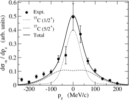
Figure 3: The longitudinal momentum distribution of the ¹⁵C fragment from the breakup reaction of ¹⁶C on ¹²C target at 83 MeV/nucleon, obtained with the parameter set D. The contribution from the 1/2⁺ and 5/2⁺ states of ¹⁵C are shown by the dotted and the dashed lines, respectively. The experimental data are taken from Ref. Y03 .

Figure 3 compares the eikonal approximation for the breakup reaction ¹⁶C + ¹²C $\to^{15}$C + $X$ at $E=83$ MeV/nucleon with the experimental data Y03 . We use the optical potential of Comfort and Karp CK80 for the neutron-¹²C potential. The optical potential between the ¹⁵C fragment and the target is constructed with the single folding procedure using the ¹⁴C density given in Ref. PZV00 and a s.p. wave function for the valence neutron for a specified final state of the fragment nucleus. As is often done, we assume that the cross sections for diffractive breakup (i.e., elastic breakup) behave exactly the same as the stripping cross sections as a function of longitudinal momentum, and thus we scale the calculated cross section (12) to match with the peak of the experimental data. The dotted and dashed lines in Fig. 3 are contribution from the 1$s_{1/2}$ and 2$d_{5/2}$ states of the fragment ¹⁵C nucleus, respectively. These are added incoherently to obtain the total one neutron removal cross section, which is denoted by the solid line. Our result reproduces remarkably well the experimental longitudinal momentum distribution of the ¹⁵C fragment in the range of $-$200MeV/c $\leq$p${}_{z}\leq$ 200MeV/c.

In summary, we have applied the $n$-$n$-¹⁴C three-body model in order to investigate the properties of the ¹⁶C nucleus. We diagonalized the three-body Hamiltonian with the finite range Minnesota potential for the interaction between the valence neutrons. As the basis states, we adopted the single-particle states obtained from the Woods-Saxon potentials, in which the continuum spectrum is discretized within the large box. With this model, the experimental data for the root-mean-square radius, the B(E2) value from the first 2⁺ state to the ground state, and the longitudinal momentum distribution of the ¹⁵C fragment from ¹⁶C breakup are all reproduced well. In particular, we have succeeded to reproduce the B(E2) value for both ¹⁵C and ¹⁶C nuclei simultaneously using the core polarization charge which is consistent with the one obtained with the particle-vibration coupling models. The calculated probability of the (1d${}_{5/2})^{2}$ configuration in the ground state wave function of ¹⁶C is about 70% while that of the (2s${}_{1/2})^{2}$ configuration is about 18%. These values are close to those extracted from the analyses of the experimental longitudinal momentum distribution.

We thank W. Horiuchi, C.A. Bertulani, and N. Vinh Mau for useful discussions. We also thank T. Yamaguchi for sending us the experimental data in a numerical form. This work was supported by the Japanese Ministry of Education, Culture, Sports, Science and Technology by Grant-in-Aid for Scientific Research under the program numbers (C(2)) 16540259 and 16740139.

References

- (1) M. Matsuo, Nucl. Phys. A696, 371 (2001).
- (2) N. Imai et al., Phys. Rev. Lett. 92, 062501 (2004).
- (3) Z. Elekes et al., Phys. Lett. B586, 34 (2004).
- (4) H.J. Ong et al., Phys. Rev. C73, 024610 (2006).
- (5) Y. Kanada-En’yo, Phys. Rev. C71, 014310 (2005).
- (6) H. Sagawa, X.R. Zhou, X.Z. Zhang, and T. Suzuki, Phys. Rev. C70, 054316 (2004).
- (7) G. Thiamova, N. Itagaki, T. Otsuka, and K. Ikeda, Eur. Phys. J. A22, 461 (2004).
- (8) Y. Suzuki, H. Matsumura, and B. Abu-Ibrahim, Phys. Rev. C70, 051302(R) (2004).
- (9) W. Horiuchi and Y. Suzuki, Phys. Rev. C73, 037304 (2006); ibid. 74, 019901 (2006).
- (10) S. Fujii et al., e-print: nucl-th/0602002.
- (11) M. Yamagami, Phys. Rev. C72, 064308 (2005).
- (12) G.F. Bertsch and H. Esbensen, Ann. Phys. (N.Y.) 209, 327 (1991).
- (13) H. Esbensen, G.F. Bertsch and K. Hencken, Phys. Rev. C56, 3054 (1999).
- (14) N. Vinh Mau and J.C. Pacheco, Nucl. Phys. A607, 163 (1996).
- (15) K. Hagino and H. Sagawa, Phys. Rev. C72, 044321 (2005).
- (16) K. Hagino, H. Sagawa, J. Carbonell and P. Schuck, e-print: nucl-th/0611064.
- (17) N. Vinh Mau, Nucl. Phys. A592, 33 (1995).
- (18) R. Thompson, M. Lemere, and Y.C. Tang, Nucl. Phys. A286, 53 (1977).
- (19) T. Zheng et al., Nucl. Phys. A709, 103 (2002).
- (20) V. Maddalena et al., Phys. Rev. C63, 024613 (2001).
- (21) T. Yamaguchi et al., Nucl. Phys. A724, 3 (2003).
- (22) D.M. Brink and R.A. Broglia, Nuclear Superfluidity: Pairing in Finite Systems, (Cambridge University Press, Cambridge, 2005).
- (23) F. Azjenberg-Selove, Nucl. Phys. A523, 1 (1991).
- (24) A. Bohr and B.R. Mottelson, Nuclear Structure, (W.A. Benjamin, Reading, MA, 1975), Vol. II.
- (25) H. Sagawa and K. Asahi, Phys. Rev. C63, 064310 (2001).
- (26) T. Suzuki, H. Sagawa, and K. Hagino, Phys. Rev. C68, 014317 (2003).
- (27) M.S. Hussein and K.W. McVoy, Nucl. Phys. A445, 124 (1985).
- (28) K. Hencken, G. Bertsch, and H. Esbensen, Phys. Rev. C54, 3043 (1996).
- (29) H. Esbensen, Phys. Rev. C53, 2007 (1996).
- (30) C.A. Bertulani and P.G. Hansen, Phys. Rev. C70, 034609 (2004); C.A. Bertulani and A. Gade, Comp. Phys. Comm. 175, 372 (2006).
- (31) J.R. Comfort and B.C. Karp, Phys. Rev. C21, 2162 (1980).
- (32) Yu.L. Parfenova, M.V. Zhukov, and J.S. Vaagen, Phys. Rev. C62, 044602 (2000).