Behaviour of the $\Lambda N$- and $\Lambda NN$- potential strengths in the ${}_{\Lambda}^{5}$He hypernucleus

Abstract

Variational study of the ${}_{\Lambda}^{5}$He hypernucleus is presented using a realistic Hamiltonian and a fully correlated wave function including $\Lambda N$ space-exchange correlations. Behaviour of $\Lambda$-separation energy ($B_{\Lambda}$) with two- and three- baryon potential strengths is thoroughly investigated. Solutions for these potential strengths giving experimental $B_{\Lambda}$ are presented.

Recently, a variational study AAU06 of the ${}_{\Lambda}^{5}$He hypernucleus has been performed with a realistic Hamiltonian and a fully correlated wave function (WF). The WF takes into account all relavant dynamical correlations induced by the two- and three- baryon potentials and the $\Lambda N$ space-exchange correlation ($SEC$) that arises due to the space-exchange potential. The findings of the investigation suggest that no realistic study ignoring $SEC$ is fair as it significantly affects every physical observable like energy breakdown, $\Lambda$-separation energy ($B_{\Lambda}$), nuclear core polarization ($NCP$), point proton radius and density profiles. The effect is found more evident in the ${}_{\Lambda\Lambda}^{\>\>\>6}$He double-$\Lambda$ hypernucleus AAU206 . The ground-state energy of the hypernucleus ($E$) or the $\Lambda$-separation energy ($B_{\Lambda}=E_{{}^{4}{\rm He}}-E$) depends on the strengths of the potentials involved in the Hamiltonian.

A realistic Hamiltonian $H$ of the hypernucleus, is written as a sum of the Hamiltonians due to the nuclear core ($NC$) of the hypernucleus ($H_{NC}$) and due to the $\Lambda$-baryon ($H_{\Lambda}$),

$$H = H_{NC}+H_{\Lambda},$$ (1)

$$H_{NC} = T_{NC}+\sum_{i<j}v_{ij}+\sum_{i<j<k}V_{ijk},$$ (2)

$$H_{\Lambda} = T_{\Lambda}+\sum_{i}v_{\Lambda i}+\sum_{i<j}V_{\Lambda ij}.$$ (3)

Here, subscripts $i,j$ and $k$ refer to nucleons. For the $S=0$ sector, we use Argonne $v_{18}$ $NN$ potential AV18 and Urbana type $NNN$ potential NNN-IX ; NNN , which successfully explain the nuclear energy spectra and are well established. However, for the $S=-1$ sector, $\Lambda N$ and $\Lambda NN$ potential strengths are yet to be determined. The dependence of energy on these strengths is the theme of this work.

Variation in any of the potential strengths would directly affect the expectation value of the respective potential. It would also affect the WF as correlations are a solutions of these potentials. Moreover, there are sensitivities to operators among various terms of the Hamiltonian and the correlation functions. Correlations like $SEC$ bring-in changes in the density profiles which affect even the central pieces of the energy breakdown. The basic ingredients like these strengths, therefore affect the ground-state energy collectively. It would not be possible to perform a proper study for a particular potential strength ignoring others. Thus, in order to pin down these potential strengths, we have to handle them all together. The energy of ${}_{\Lambda}^{5}$He is thoroughly investigated along these lines. Such a study of all the s-shell single- and double-$\Lambda$ hypernuclei may help to pin down these strengths, which, in turn, may resolve the outstanding $A=5$ anomaly DHT72 ; Gal75 ; Hungerford84 with no additional effort. Thus the present investigation is a step forward to answer, (i) whether we can successfully reproduce the hypernuclear energy spectra using these potentials without invoking the underlying Quantum Chromodynamics? (ii) and whether there is a possibility of physical existence of a bound ($I=0,J=1^{+}$) ${}_{\Lambda\Lambda}^{\;\;\;4}$H hypernucleus which has been recently conjectured Ahn01 ? This would be helpful in studying the heavy hypernuclei specially ${}_{\>\>\>\>\Lambda}^{209}$Pb whose core density matches the nuclear matter density. Hence, this would lead us to investigate, in detail, the physics of charmed and bottom hypernuclei Tyapkin ; Dover ; Khanna as well as to the nature and structure of neutron stars.

The $\Lambda NN$ potential arises from projecting out $\Sigma$, $\Delta$, etc., degrees of freedom from a coupled channel formalism. This is written as a sum of two terms, $V_{\Lambda ij}=V_{\Lambda ij}^{D}+V_{\Lambda ij}^{2\pi}$, as in Fig. 1. The dispersive potential $V_{\Lambda ij}^{D}$, arising from the suppression mechanism owing to $\Lambda N-\Sigma N$ coupling BR70 ; BR71 ; Rozynek79 ; UB99 , is written including the explicit spin dependence as BU88

$$V_{\Lambda ij}^{D}=W^{D}T_{\pi}^{2}(m_{\pi}r_{\Lambda i})T_{\pi}^{2}(m_{\pi}r_{\Lambda j})[1+\mbox{\boldmath$\sigma$}_{\Lambda}\cdot(\mbox{\boldmath$\sigma$}_{i}+\mbox{\boldmath$\sigma$}_{j})/6].$$ (4)

However, spin term is too weak for spin zero core nucleus. Here, $W^{D}$ is the strength. The $V_{\Lambda ij}^{2\pi}$ is a two-pion exchange attractive potential. Neglecting higher partial waves it is written as a sum of two terms representing p- and s-wave $\pi-N$ scatterings, $V_{\Lambda ij}^{2\pi}=V_{\Lambda ij}^{P}+V_{\Lambda ij}^{S}$ as in Ref. Bhaduri67 . The explicit form of these potentials are

$$V^{P}_{\Lambda ij}=-\left(C^{P}/6\right)(\mbox{\boldmath$\tau$}_{i}\cdot\mbox{\boldmath$\tau$}_{j})\{X_{i\Lambda},X_{\Lambda j}\},$$ (5)

and

$$V^{S}_{\Lambda ij} = C^{S}Z(m_{\pi}r_{i\Lambda})Z(m_{\pi}r_{j\Lambda})\mbox{\boldmath$\sigma$}_{i}\cdot{\hat{\bf r}}_{i\Lambda}\mbox{\boldmath$\sigma$}_{j}\cdot{\hat{\bf r}}_{j\Lambda}\mbox{\boldmath$\tau$}_{i}\cdot\mbox{\boldmath$\tau$}_{j}$$ (6)

$$\equiv C^{S}O_{\Lambda ij}^{S}$$

with

$$X_{\Lambda i}=(\mbox{\boldmath$\sigma$}_{\Lambda}\cdot\mbox{\boldmath$\sigma$}_{i})Y_{\pi}(m_{\pi}r_{\Lambda i})+S_{\Lambda i}T_{\pi}(m_{\pi}r_{\Lambda i})$$ (7)

and

$$Z(x)=\frac{x}{3}[Y_{\pi}(x)-T_{\pi}(x)].$$ (8)

It may be expressed as generalised tensor-tau type operators $(\mbox{\boldmath$\sigma$}_{i}\cdot{\bf r}_{\Lambda i})(\mbox{\boldmath$\sigma$}_{j}\cdot{\bf r}_{\Lambda j})$, $(\mbox{\boldmath$\sigma$}_{i}\cdot{\bf r}_{\Lambda i})(\mbox{\boldmath$\sigma$}_{j}\cdot{\bf r}_{\Lambda i})$, $(\mbox{\boldmath$\sigma$}_{i}\cdot{\bf r}_{\Lambda j})(\mbox{\boldmath$\sigma$}_{j}\cdot{\bf r}_{\Lambda j})$, and $(\mbox{\boldmath$\sigma$}_{i}\cdot\mbox{\boldmath$\sigma$}_{j})$ followed by $(\mbox{\boldmath$\tau$}_{i}\cdot\mbox{\boldmath$\tau$}_{j})$, thus has a strong tensor dependence. In the above expressions, $S_{\Lambda i}$ is the tensor operator, $Y_{\pi}(x)$ is the Yukawa function

$$Y_{\pi}(x)=\frac{e^{-x}}{x}\xi_{Y}(r),$$ (9)

and $T_{\pi}(x)$ is the one-pion exchange tensor potential

$$T_{\pi}(x) = \left(1+\frac{3}{x}+\frac{3}{x^{2}}\right)\frac{e^{-x}}{x}\xi_{T}(r).$$ (10)

Here, $\xi_{Y}(r)$ and $\xi_{T}(r)$ are short-range cut-off functions,

$$\xi_{Y}(r)=\xi_{T}^{1/2}(r)=\left(1-e^{-cr^{2}}\right).$$ (11)

Here, $c=2.0$ fm^-2 is a cut-off parameter and subscripts $i,j$ and $\Lambda$ refer to two nucleons and a $\Lambda$ in the triplet ($\Lambda ij$). The $C^{P}$ and the $C^{S}$ are the strengths of $V^{P}_{\Lambda ij}$ and $V^{S}_{\Lambda ij}$, respectively. The latter is a very weak term compared to the former. Its strength is not known experimentally. However, we may make a qualitative theoretical estimate for it by comparing the strengths of modern $NNN$ potentials obtained using $SU(3)$ symmetry. Using chiral perturbation theory, Friar et al. Friar99 have compared the modern $NNN$ potentials, namely: (i) Tucson-Melbourn Coon79 , (ii) Brazil Coelho83 , (iii) Ruhr Eden93 and (iv) Texas Kolck94 containing a $\sigma$-term for $\pi-N$ scattering. They also consider the Fujita-Miyazawa force Fujita57 dropping s-wave pions and Urbana-Argonne model NNN with additional isospin- and spin- independent components added to the Fujita-Miyazawa force.

Figure 1: Diagarm representing $V_{\Lambda NN}^{D}$ and $V_{\Lambda NN}^{2\pi}$.

In the Tucson-Melbourne (TM) model, the s-wave NNN force is written in the form

$$B({\bf r}_{ij},{\bf r}_{jk})\{\mbox{\boldmath$\tau$}_{i}\cdot\mbox{\boldmath$\tau$}_{j},\mbox{\boldmath$\tau$}_{j}\cdot\mbox{\boldmath$\tau$}_{k}\}\{(S_{ij}+\mbox{\boldmath$\sigma$}_{i}\cdot\mbox{\boldmath$\sigma$}_{j})(S_{jk}+\mbox{\boldmath$\sigma$}_{j}\cdot\mbox{\boldmath$\sigma$}_{k})\},$$ (12)

where, $B({\bf r}_{ij},{\bf r}_{jk})$ has several terms given in Ref. NNN . Recently, this has been expressed retaining only the term with pion-exchange-range functions as SCP01

$$A^{S}=\left(\frac{f_{\pi NN}}{4\pi}\right)^{2}a^{\prime}m_{\pi}^{2},$$ (13)

$$O^{S}_{ijk}=\sum_{cyc}Z(m_{\pi}r_{ij})Z(m_{\pi}r_{jk})\mbox{\boldmath$\sigma$}_{i}\cdot{\hat{\bf r}}_{ij}\mbox{\boldmath$\sigma$}_{k}\cdot{\hat{\bf r}}_{kj}\mbox{\boldmath$\tau$}_{i}\cdot\mbox{\boldmath$\tau$}_{k}.$$ (14)

The parameter $a^{\prime}$, whose value ranges from $-0.51/m_{\pi}$ to $-1.87/m_{\pi}$, is listed in Ref. Friar99 . The TM value $a^{\prime}=-1.03/m_{\pi}$ gives the strength $|A^{S}|\approx$0.8 MeV. However, in many others it is assumed to have a value of 1.0 MeV.

Comparing TM model with the Eq. 6 for $\Lambda NN$ potential, one may write an identical structure for both s-wave $\Lambda NN$ and $NNN$ potentials as following

$$C^{S}O^{S}_{\Lambda jk}\equiv A^{S}O_{ijk}.$$ (15)

This directly relates $C^{S}$ in the strange sector to $A^{S}$ in the non-strange sector. Since $\Lambda-N$ mass difference is small compared to the $\Delta-N$ mass difference, $\Lambda NN$ potential of $S=-1$ sector is stronger than its non-strange counterpart $NNN$ potential Bhaduri67 of $S=0$ sector. This provides stronger strengths in the case of $\Lambda NN$ potential compared to the $NNN$ potential. We, therefore, expect that the value of $C^{S}$ would be more than 1.0 MeV, and is taken to be 1.5 MeV.

The charge symmetric $\Lambda N$ potential BUC84 ; Lagaris81 reads as

$$v_{\Lambda N}(r)=v_{0}(r)(1-\varepsilon+\varepsilon P_{x})+(v_{\sigma}/4)T_{\pi}^{2}(m_{\pi}r)\mbox{\boldmath$\sigma$}_{\Lambda}\cdot\mbox{\boldmath$\sigma$}_{N}.$$ (16)

The first term includes direct potential ($v_{0}(r)=v_{c}(r)-v_{2\pi}(r)$) and space-exchange potential ($\varepsilon v_{0}(r)(P_{x}-1)$). Here, $\varepsilon$ determines the odd-state potential, which is the strength of the space-exchange potential relative to the direct potential. Its estimate from the $\Lambda p$ forward-backward asymmetry is poor that ranges from 0.1 to 0.38 UB99 . The potential $v_{c}(r)=W_{c}/[1+{\rm exp}\{(r-R)/ar\}]$ is the Saxon-Woods repulsive potential, with $W_{c}=2137$ MeV, $R=0.5$ fm and $a=0.2$ fm, and $v_{2\pi}=\overline{v}T_{\pi}^{2}(m_{\pi}r)$ is the two-pion attractive potential. The constants, $\overline{v}=(v_{s}+3v_{t})/4$ and $v_{\sigma}=v_{s}-v_{t}$, are respectively the spin-average and spin-dependent strengths, with $v_{s(t)}$ the singlet(triplet) state potential depth.

Table 1: $\Lambda N$ potential strengths in units of MeV.

	$v_{s}$	$v_{t}$	$\overline{v}=(v_{s}+3v_{t})/4$	$v_{\sigma}=v_{s}-v_{t}$
$\overline{v}1$	6.33	6.09	6.15	0.24
$\overline{v}2$	6.28	6.04	6.10	0.24
$\overline{v}3$	6.23	5.99	6.05	0.24

We perform variational Monte Carlo study to calculate the ground-state energy, $E={\langle\Psi|H|\Psi\rangle}/{\langle\Psi|\Psi\rangle}$, where $\Psi$ is the WF of the hypernucleus. The computational details are available in Ref. AAU06 . For the spin-zero core nucleus, the expectation value of the spin part of the $\Lambda N$ potential is negligibly small AAU06 ; AAU03 ; UPU95 ; AAU95 . So is the s-wave part of $\Lambda NN$ potential. Moreover, correlations induced by them are too weak to offer any significant change in the energy. Thus, we choose a reasonable strength for these two. The energy is very sensitive to changes in the $\Lambda N$ potential strengths $\overline{v}$ and $\varepsilon$. They implicitly appear in the WF through the $\Lambda N$ central and the $SEC$ correlations. The $\Lambda NN$ potential and its correlations involving $C^{P}$ and $W^{D}$ play an important role. Therefore, $E$ or $B_{\Lambda}$ are sensitive to the strengths $\overline{v}$, $\varepsilon$, $C^{P}$ and $W^{D}$.

The value of $\overline{v}\approx 6.15(5)$ MeV is found consistent with the low energy $\Lambda p$ scattering data BU88 . We use three different sets of $v_{s}$ and $v_{t}$, which give three different values of $\overline{v}$ and a constant $v_{\sigma}$ as in Table 1, referred to as $\overline{v}1$, $\overline{v}2$ and $\overline{v}3$. For all these, we choose three values of $\varepsilon$ in the range from 0.1 to 0.38 as mentioned before. These are 0.1, 0.2 and 0.3. Results for these values are given in Tables 2, 3 and 4.

The correlations induced by different components of $\Lambda NN$ potential is written using scaled pair distances ($\overline{r}$) and a variational parameter $\delta^{m}$ as in Ref. AAU03 ,

$$U_{\Lambda ij}=\sum_{m}U_{\Lambda ij}^{m}=\sum_{m=D,P,S}\delta^{m}V^{m}(\overline{r}_{\Lambda i},\overline{r}_{ij},\overline{r}_{j\Lambda}).$$ (17)

The $\langle V^{D}_{\Lambda ij}\rangle$ obeys a linear behaviour, $\partial V^{D}_{\Lambda ij}/\partial W^{D}=\partial E/\partial W^{D}$=constant at a fixed $\varepsilon$ as it is not sensitive to the operators but only to $SEC$ and hence to $\varepsilon$. As is obvious from Eq. 17, a change in the strength $C^{P}$ offsets the WF. We observe that along with its own correlation parameter $\delta^{P}$ a couple of other parametres are found to change with $C^{P}$. But the repulsive $\Lambda NN$ correlation, $U_{\Lambda NN}^{D}$, remains invariant. We perform calculations for a wide range of $C^{P}$ starting from 0.5 MeV and upto 2.0 MeV. Therefore, enhancements in the attraction due to increasing $C^{P}$ needs to be balanced by an appropriate increase in $W^{D}$. For every independent calculation, we tune the WF afresh and adjust the repulsive strength $W^{D}$ in order to reproduce the experimental $B_{\Lambda}$. For the new $W^{D}(new)$, we may easily obtain new $\delta^{D}(new)$ using

$$\delta^{D}(old)W^{D}(old)=\delta^{D}(new)W^{D}(new),$$ (18)

as $U^{D}_{\Lambda NN}$ is constant with $C^{P}$. Thus $\delta^{D}$ decreases in the same proportion $W^{D}$ increases. The same is not true in the case of $\delta^{P}$, which is found to be alomst constant even if we multiply $C^{P}$ by a factor of 4. This is because of the sensitivity of $V^{P}_{\Lambda ij}$ to its correlation, which is so strong that the attraction, $\langle V_{\Lambda ij}^{2\pi}\rangle$, increases more than 12 times for the corresponding 4 times increase in $C^{P}$. This quadratic behaviour is observed for all the $\varepsilon$ and all the $\overline{v}$. The respective increase in the $NC$ part of the energy ($E_{NC}$) is about 4 MeV. The $T_{\Lambda}$ and $v_{\Lambda i}$ also exhibit considerable change due to the variation in $C^{P}$.

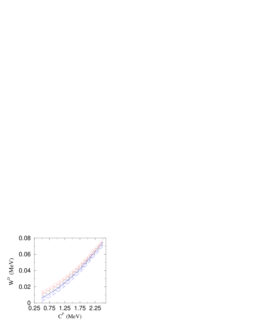
Figure 2: Curves show the set of strengths giving $B_{\Lambda}^{exp}$. The dotted, dashed and long dashed lines represent $\varepsilon$=0.1, 0.2 and 0.3, and the red, black and blue colors represent $\overline{v}1$, $\overline{v}2$ and $\overline{v}3$, respectively.

Solutions of all these strengths reproducing $B_{\Lambda}^{exp}$ are plotted in Fig. 2. Thus, following the curves one may find potential strengths that reproduce $B_{\Lambda}^{exp}$. For every $\overline{v}$ and at a fix value of $C^{P}$, we observe a linear realtionship, ${\partial W^{D}}/{\partial\varepsilon}\approx c$, which is a consequence of two other linear relationships: (i) ${\partial E}/{\partial\varepsilon}=-{\partial B_{\Lambda}}/{\partial\varepsilon}\approx c_{1}$ (ii) and ${\partial V^{D}_{\Lambda ij}}/{\partial W^{D}}=-{\partial E}/{\partial W^{D}}={\partial B_{\Lambda}}/{\partial W^{D}}\approx c_{2}$. The slope, $c=c_{1}/c_{2}$ is found to increases with $C^{P}$, but only slightly (Table 5). Curves representing different $\overline{v}$ are found to get closer at higher $C^{P}$. Because, the dependence of energy on $C^{P}$ as well as on $W^{D}$ varies with $\overline{v}$. To match an increase in the attractive $C^{P}$ we require a larger increase in the repulsive $W^{D}$ for smaller $\overline{v}$.

This study has established the value of parameters appearing in the two- and three-body potentials in the strange sector. Furthermore, range of variations of these parameters is now, atleast roughly, known. In order to establish these parameters over a range of hypernuclei, numerous light and heavy hypernuclei have to be studied. This would help us to understand the variation of $\Lambda N$ and $\Lambda NN$ potentials as a function of density. Such a study would be in parallel to that of $NN$ and $NNN$ potentials in nuclear systems where density variation plays an important role. A proper understanding of hypernuclei would help us to clarify the behaviour of the nuclear forces in the strange sector. Ultimately, a detailed study may lead us to a clarification of the role of QCD in determining the potential strengths. New results expected from Japan Hadron Facility would help to sort out these questions in the near future.

The work is supported under Grant No. SP/S2/K-32/99 awarded to AAU by the Department of Science and Technology, Government of India. FCK thanks NSERCC for financial support.

Table 2: Energy breakdown for the set $\overline{v}1$ ($\overline{v}=6.15$ and $v_{\sigma}=0.24$). All quantities are in units of MeV except for $\varepsilon$.

	$\varepsilon=0.1$				$\varepsilon=0.2$				$\varepsilon=0.3$
	$C^{p}=.5$	$C^{p}=1.0$	$C^{p}=1.5$	$C^{p}=2.0$	$C^{p}=.5$	$C^{p}=1.0$	$C^{p}=1.5$	$C^{p}=2.0$	$C^{p}=.5$	$C^{p}=1.0$	$C^{p}=1.5$	$C^{p}=2.0$
$T_{\Lambda}$	8.56(3)	8.97(3)	9.83(3)	10.46(4)	8.23(3)	8.76(3)	9.38(3)	10.02(4)	7.94(3)	8.39(3)	9.01(3)	9.58(3)
$v_{0}(r)(1-\varepsilon)$	-16.08(6)	-16.36(6)	-16.78(6)	-17.03(6)	-13.69(5)	-14.07(5)	-14.37(5)	-14.51(5)	-11.55(4)	-11.91(4)	-12.06(4)	-12.22(5)
$v_{0}(r)\varepsilon P_{x}$	-1.56(1)	-1.58(1)	-1.61(1)	-1.63(1)	-2.97(1)	-3.04(1)	-3.09(1)	-3.11(1)	-4.27(2)	-4.40(2)	-4.43(2)	-4.47(2)
$(\frac{1}{4})v_{\sigma}T_{\pi}^{2}(r)\mbox{\boldmath$\sigma$}_{\Lambda}\cdot\mbox{ \boldmath$\sigma$}_{i}$	0.014(0)	0.015(0)	0.017(0)	0.017(0)	0.012(0)	0.013(0)	0.014(0)	0.014(0)	0.009(0)	0.010(0)	0.011(0)	0.011(0)
$v_{\Lambda i}$	-17.63(6)	-17.93(6)	-18.38(6)	-18.65(7)	-16.65(6)	-17.10(6)	-17.42(6)	-17.61(7)	-15.80(6)	-16.30(6)	-16.48(6)	-16.68(7)
$V_{\Lambda ij}^{D}$	2.49(1)	4.60(1)	7.99(4)	12.17(6)	2.16(1)	4.20(1)	7.35(4)	11.53(6)	1.80(1)	3.81(1)	6.81(4)	10.65(5)
$V_{\Lambda ij}^{P}$	-1.36(1)	-4.40(2)	-10.02(4)	-15.99(6)	-1.36(1)	-4.54(2)	-9.42(4)	-15.35(6)	-1.28(1)	-4.16(2)	-8.97(4)	-14.38(6)
$V_{\Lambda ij}^{S}$	-0.025(0)	0.017(1)	0.066(1)	0.100(1)	-0.025(0)	0.009(1)	0.057(1)	0.087(1)	-0.030(1)	0.009(1)	0.050(1)	0.077(1)
$V_{\Lambda ij}^{2\pi}$ $=V_{\Lambda ij}^{P}+V_{\Lambda ij}^{S}$	-1.38(1)	-4.39(2)	-9.95(4)	-15.89(6)	-1.39(1)	-4.52(2)	-9.36(4)	-15.26(6)	-1.31(1)	-4.16(2)	-8.92(4)	-14.30(6)
$V_{\Lambda ij}=V_{\Lambda ij}^{D}+V_{\Lambda ij}^{2\pi}$	1.11(1)	0.21(2)	-1.96(2)	-3.73(3)	0.77(1)	-0.33(2)	-2.05(2)	-3.73(3)	0.49(1)	-0.34(2)	-2.11(2)	-3.65(3)
$V_{\Lambda}{}=v_{\Lambda i}+V_{\Lambda ij}$	-16.52(6)	-17.72(6)	-20.34(6)	-22.38(7)	-15.88(6)	-17.43(6)	-19.43(6)	-21.34(7)	-15.31(6)	-16.64(6)	-18.59(6)	-20.33(7)
$E_{\Lambda}=T_{\Lambda}+V_{\Lambda}$	-7.96(3)	-8.75(4)	-10.51(4)	-11.92(5)	-7.64(4)	-8.67(4)	-10.05(4)	-11.32(5)	-7.37(4)	-8.26(4)	-9.58(4)	-10.75(5)
$T_{NC}$	117.59(15)	118.42(15)	118.69(15)	119.26(15)	116.97(15)	117.84(15)	118.42(15)	118.84(15)	117.51(15)	118.43(15)	118.07(15)	118.53(15)
$v_{NN}$	-134.65(14)	-134.53(14)	-133.18(14)	-132.55(14)	-134.36(14)	-134.05(14)	-133.41(14)	-132.79(14)	-134.99(14)	-134.85(14)	-133.42(14)	-132.87(14)
$V_{NNN}$	-5.81(2)	-5.98(2)	-5.84(2)	-5.66(2)	-5.82(2)	-5.97(2)	-5.83(2)	-5.67(2)	-5.99(2)	-6.15(2)	-5.93(2)	-5.76(2)
$V_{NC}=v_{ij}+V_{ijk}$	-140.46(14)	-140.51(14)	-139.02(14)	-138.21(14)	-140.16(14)	-140.03(14)	-139.24(14)	-138.46(14)	-140.98(14)	-141.00(14)	-139.35(14)	-138.63(14)
$E_{NC}=T_{NC}+V_{NC}$	-22.88(4)	-22.10(5)	-20.32(4)	-18.95(5)	-23.21(4)	-22.18(5)	-20.82(4)	-19.52(5)	-23.47(4)	-22.58(5)	-21.27(4)	-20.11(5)
$E=E_{\Lambda}+E_{NC}$	-30.84(2)	-30.85(2)	-30.84(3)	-30.87(4)	-30.85(2)	-30.85(2)	-30.86(3)	-30.84(4)	-30.84(2)	-30.84(2)	-30.86(3)	-30.86(4)

Table 3: Energy breakdown for the set $\overline{v}2$ ($\overline{v}=6.10$ and $v_{\sigma}=0.24$). All quantities are in units of MeV except for $\varepsilon$.

	$\varepsilon=0.1$				$\varepsilon=0.2$				$\varepsilon=0.3$
	$C^{p}=.5$	$C^{p}=1.0$	$C^{p}=1.5$	$C^{p}=2.0$	$C^{p}=.5$	$C^{p}=1.0$	$C^{p}=1.5$	$C^{p}=2.0$	$C^{p}=.5$	$C^{p}=1.0$	$C^{p}=1.5$	$C^{p}=2.0$
$T_{\Lambda}$	8.09(3)	8.54(3)	9.19(3)	9.91(3)	7.80(3)	8.15(3)	8.65(3)	9.51(3)	7.57(3)	7.94(3)	8.44(3)	9.18(3)
$v_{0}(r)(1-\varepsilon)$	-14.61(5)	-14.79(5)	-15.13(5)	-15.48(5)	-12.54(5)	-12.64(5)	-12.94(5)	-13.30(5)	-10.59(4)	-10.73(4)	-11.04(5)	-11.15(4)
$v_{0}(r)\varepsilon P_{x}$	-1.41(1)	-1.42(1)	-1.45(1)	-1.47(1)	-2.70(1)	-2.72(1)	-2.77(1)	-2.83(1)	-3.88(2)	-3.93(2)	-4.03(2)	-4.03(2)
$(\frac{1}{4})v_{\sigma}T_{\pi}^{2}(r)\mbox{\boldmath$\sigma$}_{\Lambda}\cdot\mbox{ \boldmath$\sigma$}_{i}$	0.007(0)	0.007(0)	0.008(0)	0.009(0)	0.007(0)	0.008(0)	0.008(0)	0.009(0)	0.005(0)	0.005(0)	0.006(0)	0.007(0)
$v_{\Lambda i}$	-16.02(6)	-16.20(6)	-16.57(6)	-16.94(6)	-15.23(6)	-15.35(6)	-15.70(6)	-16.12(6)	-14.46(6)	-14.65(6)	-15.04(6)	-15.18(6)
$V_{\Lambda ij}^{D}$	1.65(1)	3.46(2)	6.43(4)	10.39(5)	1.32(1)	3.09(2)	5.95(4)	9.81(5)	0.99(1)	2.71(2)	5.47(4)	9.22(5)
$V_{\Lambda ij}^{P}$	-1.33(1)	-4.36(2)	-9.00(4)	-14.95(6)	-1.23(1)	-4.04(2)	-8.08(3)	-14.26(6)	-1.19(1)	-3.98(2)	-7.61(3)	-13.84(6)
$V_{\Lambda ij}^{S}$	-0.028(0)	0.014(1)	0.049(1)	0.087(0)	-0.035(0)	0.007(0)	0.040(1)	0.078(0)	-0.032(0)	0.009(0)	0.036(1)	0.074(0)
$V_{\Lambda ij}^{2\pi}$ $=V_{\Lambda ij}^{P}+V_{\Lambda ij}^{S}$	-1.35(1)	-4.35(2)	-8.59(4)	-14.86(6)	-1.27(1)	-4.04(2)	-8.04(4)	-14.18(6)	-1.22(1)	-3.97(2)	-7.80(4)	-13.77(6)
$V_{\Lambda ij}=V_{\Lambda ij}^{D}+V_{\Lambda ij}^{2\pi}$	-0.30(1)	-0.88(2)	-2.53(2)	-4.47(3)	0.05(1)	-0.94(2)	-2.09(2)	-4.37(3)	0.49(1)	-1.26(2)	-2.33(2)	-4.55(3)
$V_{\Lambda}{}=v_{\Lambda i}+V_{\Lambda ij}$	-15.72(6)	-17.08(6)	-19.10(6)	-21.41(6)	-15.18(6)	-16.29(6)	-17.79(6)	-20.49(6)	-14.69(6)	-15.91(6)	-17.37(6)	-19.73(6)
$E_{\Lambda}=T_{\Lambda}+V_{\Lambda}$	-7.62(3)	-8.54(4)	-9.90(4)	-11.51(5)	-7.37(3)	-8.14(4)	-9.15(4)	-10.98(5)	-7.13(4)	-7.97(4)	-8.93(4)	-10.54(5)
$T_{NC}$	116.82(15)	116.53(15)	117.36(15)	118.09(15)	116.73(15)	116.68(15)	117.19(15)	117.55(15)	116.81(15)	117.03(15)	117.16(15)	117.40(15)
$v_{NN}$	-134.22(14)	-132.90(14)	-132.59(14)	-131.80(14)	-134.40(14)	-133.50(14)	-133.12(14)	-131.82(14)	-134.43(14)	-133.72(14)	-133.12(14)	-131.96(14)
$V_{NNN}$	-5.83(2)	-5.92(2)	-5.74(2)	-5.62(2)	-5.81(2)	-5.90(2)	-5.78(2)	-5.60(2)	-6.10(2)	-6.21(2)	-5.94(2)	-5.73(2)
$V_{NC}=v_{ij}+V_{ijk}$	-140.05(14)	-138.82(15)	-139.31(15)	-137.42(14)	-140.21(14)	-139.41(14)	-138.90(15)	-137.42(14)	-140.53(14)	-139.93(15)	-133.12(15)	-137.69(14)
$E_{NC}=T_{NC}+V_{NC}$	-23.22(4)	-22.31(5)	-20.97(5)	-19.32(5)	-23.47(4)	-22.71(5)	-21.71(5)	-19.87(5)	-23.71(4)	-22.89(4)	-21.91(4)	-20.29(5)
$E=E_{\Lambda}+E_{NC}$	-30.84(2)	-30.85(2)	-30.87(2)	-30.84(3)	-30.85(2)	-30.85(2)	-30.86(2)	-30.85(3)	-30.84(2)	-30.87(2)	-30.84(2)	-30.84(3)

Table 4: Energy breakdown for the set $\overline{v}3$ ($\overline{v}=6.05$ and $v_{\sigma}=0.24$). All quantities are in units of MeV except for $\varepsilon$.

	$\varepsilon=0.1$				$\varepsilon=0.2$				$\varepsilon=0.3$
	$C^{p}=.5$	$C^{p}=1.0$	$C^{p}=1.5$	$C^{p}=2.0$	$C^{p}=.5$	$C^{p}=1.0$	$C^{p}=1.5$	$C^{p}=2.0$	$C^{p}=.5$	$C^{p}=1.0$	$C^{p}=1.5$	$C^{p}=2.0$
$T_{\Lambda}$	7.60(3)	8.09(3)	8.66(3)	9.18(3)	7.27(3)	7.73(3)	8.14(3)	8.87(3)	7.11(3)	7.45(3)	7.90(3)	8.48(3)
$v_{0}(r)(1-\varepsilon)$	-13.26(5)	-13.57(5)	-13.69(5)	-13.95(5)	-11.20(4)	-11.48(5)	-11.64(5)	-12.02(5)	-9.58(4)	-9.68(4)	-9.90(4)	-9.94(4)
$v_{0}(r)\varepsilon P_{x}$	-1.27(1)	-1.30(1)	-1.30(1)	-1.31(1)	-2.40(1)	-2.45(1)	-2.48(1)	-2.54(1)	-3.49(2)	-3.51(2)	-3.56(2)	-3.58(2)
$(\frac{1}{4})v_{\sigma}T_{\pi}^{2}(r)\mbox{\boldmath$\sigma$}_{\Lambda}\cdot\mbox{ \boldmath$\sigma$}_{i}$	-0.003(0)	-0.002(0)	-0.002(0)	-0.001(0)	0.003(0)	0.004(0)	0.005(0)	0.006(0)	0.002(0)	0.002(0)	0.003(0)	0.003(0)
$v_{\Lambda i}$	-14.53(6)	-14.87(6)	-15.00(6)	-15.27(6)	-13.60(6)	-13.92(6)	-14.10(6)	-14.56(6)	-13.06(6)	-13.19(6)	-13.48(6)	-13.52(6)
$V_{\Lambda ij}^{D}$	0.87(0)	2.61(1)	5.30(3)	8.79(5)	0.51(0)	2.16(1)	4.68(3)	8.25(5)	0.24(0)	1.82(1)	4.31(3)	7.50(4)
$V_{\Lambda ij}^{P}$	-1.20(1)	-4.07(2)	-8.53(4)	-13.45(6)	-1.11(1)	-3.84(2)	-7.49(4)	-12.87(6)	-1.06(1)	-3.62(2)	-7.24(4)	-12.27(6)
$V_{\Lambda ij}^{S}$	-0.032(0)	0.010(0)	0.046(0)	0.071(1)	-0.037(0)	0.003(0)	0.030(0)	0.062(1)	-0.037(0)	0.001(0)	0.029(0)	0.060(1)
$V_{\Lambda ij}^{2\pi}$ $=V_{\Lambda ij}^{P}+V_{\Lambda ij}^{S}$	-1.23(1)	-4.06(2)	-6.48(4)	-13.37(6)	-1.15(1)	-3.84(2)	-7.46(4)	-12.81(6)	-1.09(1)	-3.63(2)	-7.21(4)	-12.21(6)
$V_{\Lambda ij}=V_{\Lambda ij}^{D}+V_{\Lambda ij}^{2\pi}$	-0.37(1)	-1.44(2)	-3.19(2)	-4.59(3)	-0.64(1)	-1.68(2)	-2.78(2)	-4.56(3)	-0.85(1)	-1.81(2)	-2.90(2)	-4.71(3)
$V_{\Lambda}{}=v_{\Lambda i}+V_{\Lambda ij}$	-14.89(7)	-16.32(6)	-18.19(6)	-19.86(6)	-14.24(7)	-15.60(6)	-16.89(6)	-19.12(6)	-13.91(7)	-11.48(6)	-16.38(6)	-18.23(6)
$E_{\Lambda}=T_{\Lambda}+V_{\Lambda}$	-7.29(3)	-8.23(3)	-9.52(4)	-10.67(4)	-6.97(3)	-7.87(4)	-8.75(4)	-10.25(4)	-6.80(3)	-7.55(4)	-8.48(4)	-9.74(4)
$T_{NC}$	115.97(15)	116.33(15)	116.54(15)	116.42(15)	115.28(15)	115.70(15)	116.01(15)	116.81(15)	116.04(15)	116.28(15)	116.23(15)	115.68(15)
$v_{NN}$	-133.81(14)	-133.07(14)	-132.06(14)	-131.98(14)	-133.44(14)	-132.81(14)	-132.32(14)	-131.73(14)	-134.04(14)	-133.41(14)	-132.63(14)	-131.08(14)
$V_{NNN}$	-5.73(2)	-5.88(2)	-5.80(2)	-5.61(2)	-5.73(2)	-5.87(2)	-5.75(2)	-5.67(2)	-6.03(2)	-6.16(2)	-5.95(2)	-5.71(2)
$V_{NC}=v_{ij}+V_{ijk}$	-139.53(14)	-138.95(14)	-137.86(14)	-136.59(14)	-139.17(14)	-138.68(14)	-138.07(14)	-137.40(14)	-140.08(14)	-139.57(14)	-138.58(14)	-136.79(14)
$E_{NC}=T_{NC}+V_{NC}$	-23.57(4)	-22.61(5)	-21.32(4)	-20.17(5)	-23.89(4)	-22.98(4)	-22.09(4)	-20.59(5)	-24.04(4)	-23.29(4)	-22.36(4)	-21.11(5)
$E=E_{\Lambda}+E_{NC}$	-30.85(2)	-30.84(2)	-30.84(2)	-30.84(3)	-30.85(2)	-30.85(2)	-30.84(2)	-30.84(3)	-30.84(2)	-30.84(2)	-30.85(2)	-30.86(3)

Table 5: Variation of the slope, $\partial W^{D}/\partial\varepsilon$, with $C^{P}$ and $\overline{v}$.

$C^{P}$ (MeV)	$\overline{v}1$ (MeV)	$\overline{v}2$ (MeV)	$\overline{v}3$ (MeV)
0.5	-0.016(1)	-0.017(1)	-0.017(1)
1.0	-0.017(1)	-0.019(1)	-0.019(1)
1.5	-0.019(1)	-0.022(1)	-0.023(1)
2.0	-0.021(1)	-0.023(1)	-0.024(1)
2.5	-0.022(1)	-0.025(1)	-0.026(1)

References

- (1) A. A. Usmani, Phys. Rev. C73, 011302(R) (2006).
- (2) A. A. Usmani and Z. Hasan, submitted to Phys. Rev. C.
- (3) R. B. Wiringa, V. G. J. Stoks, and R. Schiavilla, Phys. Rev. C51, 38 (1995).
- (4) B. S. Pudliner, V. R. Pandharipande, J. Carlson and R. B. Wiringa, Phys. Rev. Lett. 74, 4396 (1995).
- (5) J. Carlson, V. R. Pandharipande and R. B. Wiringa, Nucl. Phys. A401, 59 (1983).
- (6) R. H. Dalitz, R. C. Herndon and Y. C. Tang, Nucl. Phys. B47, 109 (1972).
- (7) A. Gal, Adv. Nucl. Phys. 8, 1 (1975).
- (8) E. V. Hungerford and L. C. Biedenhorn, Phys. Lett. 142B, 232 (1984).
- (9) K. Ahn et al., Phys. Rev. Lett 87, 132504 (2001).
- (10) A. A. Tyapkin, Sov. J. Nucl. Phys. 22, 89 (1976).
- (11) C. B. Dover and S. H. Kahana, Phys. Rev. Lett. 39, 1506 (1977).
- (12) K. Tsushima and F. C. Khanna, Phys. Rev. C67, 015211 (2003).
- (13) A. R. Bodmer, D. M. Rote and A. L. Mazza, Phys. Rev. C2, 1623 (1970).
- (14) A. R. Bodmer and D. M. Rote Nucl. Phys. A169, 1 (1971).
- (15) J. Rozynek and J. Dabrowski, Phys. Rev. C20, 1612 (1979); 23, 1706(1981); Y. Yamamoto and H. Bando, Suppl. Prog. Theor. Phys. Suppl. 81, 9(1985); Y. Yamamoto, Nucl. Phys. A450, 275c (1986).
- (16) Q. N. Usmani and A. R. Bodmer, Phys. Rev. C60, 055215 (1999).
- (17) A. R. Bodmer and Q. N. Usmani, Nucl. Phys. A477, 621 (1988).
- (18) R. K. Bhaduri, B. A. Loiseau and Y. Nogami, Anns. Phys. (N. Y) 44, 57 (1967).
- (19) J. L. Friar, D. Hüber and U. van Kolck, Phys. Rev. C59, 53 (1999).
- (20) S. A. Coon, M. D. Scadron, P. C. McNamee, B. R. Barrett, D. W. E. Blatt and B. H. J. McKellar, Nucl. Phys. A317, 242 (1979).
- (21) H. T. Coelho, T. K. Das and M. R. Robilotta, Phys. Rev. C28, 1812 (1983); M. R. Robilotta and H. T. Coelho, Nucl. Phys. A460, 645 (1986).
- (22) J. A. Eden and M. F. Gari, Phys. Rev. C53, 1510 (1996).
- (23) C. Ordóñez and U. van Kolck, Phys. Lett. B 291, 459 (1992); U. van Kolck, Phys. Rev. C49, 2932 (1994).
- (24) J.-I Fujita and H. Miyazawa, Prog. Theor. Phys. 17, 360 (1957).
- (25) S. C. Pieper, V. R. Pandharipande, R. B. wiringa and J. Carlson, Phys. Rev. C64, 014001 (2001).
- (26) A. R. Bodmer and Q. N. Usmani and J. Carlson, Phys. Rev. C29, 684 (1984).
- (27) I. E. Lagaris and V. R. Pandharipande, Nucl. Phys. A359, 331 (1981).
- (28) A. A. Usmani and S. Murtaza, Phys. Rev. C68, 024001 (2003).
- (29) A. A. Usmani, S. C. Pieper and Q. N. Usmani, Phys. Rev. C51, 2347 (1995).
- (30) A. A. Usmani, Phys. Rev. C52, 1773, (1995).