Dynamical Freeze-out in 3-Fluid Hydrodynamics

Abstract

Freeze-out procedure accepted in the model of 3-fluid dynamics (3FD) 3FD is analyzed. This procedure is formulated in terms of drain terms in hydrodynamic equations. Dynamics of the freeze-out is illustrated by 1-dimensional simulations. It is demonstrated that the resulting freeze-out reveals a nontrivial dynamics depending on initial conditions in the expanding “fireball”. The freeze-out front is not defined just “geometrically” on the condition of the freeze-out criterion met but rather is a subject the fluid evolution. It competes with the fluid flow and not always reaches the place where the freeze-out criterion is met. Dynamics of the freeze-out in 3D simulations is analyzed. It is demonstrated that the late stage of central nuclear collisions at top SPS energies is of the form of three (two baryon-rich and one baryon-free) fireballs separated from each other.

I Introduction

Hydrodynamics is now a conventional approach to simulations of heavy-ion collisions. Even review papers Clare ; Stoecker86 ; MRS91 ; Rischke98 ; Ruuskanen06 do not comprise a complete list of numerous applications of this approach. The hydrodynamics is applicable to description of hot and dense stage of nuclear matter, when the mean free path is well shorter than the size of the system. However, as expansion proceeds, the system becomes dilute, the mean free path becomes comparable to the system size, and hence the hydrodynamic calculation should be stopped at some instant. All hydrodynamic calculations are terminated by a freeze-out procedure, while these freeze-out prescriptions are somewhat different in different models.

In the present paper we would like to describe in more detail the freeze-out procedure accepted in recently developed 3FD model 3FD ; 3FDm . The 3FD model is designed for simulating heavy-ion collisions in the energy range from BNL Alternating Gradient Synchrotron (AGS) to CERN Super Proton Synchrotron (SPS). Unlike the conventional hydrodynamics, where local instantaneous stopping of projectile and target matter is assumed, a specific feature of the dynamic 3-fluid description is a finite stopping power resulting in a counter-streaming regime of leading baryon-rich matter. The basic idea of a 3-fluid approximation to heavy-ion collisions 3FD ; 3FDm is that at each space-time point a generally nonequilibrium distribution function of baryon-rich matter, can be represented as a sum of two distinct locally equilibrated contributions, initially associated with constituent nucleons of the projectile (p) and target (t) nuclei. In addition, newly produced particles, populating the mid-rapidity region, are associated with a “fireball” (f) fluid. This model is a straightforward extension of the 2-fluid model with radiation of direct pions MRS91 ; MRS88 ; INNTS and (2+1)-fluid model Kat93 ; Brac97 ; Brac00a . In particular, the 3FD model allows a certain formation time for the fireball-fluid production, during which the matter of the fluid propagates without interactions.

We have started our simulations 3FD ; 3FDflow ; 3FDpt with a simple hadronic equation of state (EoS) gasEOS . This EoS is a natural reference point for any other more elaborate EoS. The 3FD model turned out to be able to reasonably reproduce a large body of experimental data 3FD ; 3FDflow ; 3FDpt in a wide energy range from AGS to SPS. This was done with the unique set of model parameters summarized in Ref. 3FD . Problems were met in description of transverse flow 3FDflow . The directed flow required a softer EoS at top AGS and SPS energies (in particular, this desired softening may signal occurrence of a transition into quark-gluon phase).

In particular, transverse-mass spectra of various hadrons were reproduced 3FD ; 3FDpt . Experimental data on transverse-mass spectra of kaons produced in central Au+Au E866 or Pb+Pb NA49 collisions reveal peculiar dependence on the incident energy. The inverse-slope parameter (so called effective temperature) of these spectra at mid rapidity increases with incident energy in the AGS energy domain and then saturates at the SPS energies. In Refs. Gorenstein03 ; Mohanty03 it was assumed that this saturation is associated with the deconfinement phase transition. This assumption was indirectly confirmed by the fact that microscopic transport models, based on hadronic degrees of freedom, failed to reproduce the observed behavior of the kaon inverse slope Bratkovskaya . Hydrodynamic simulations of Ref. Hama04 succeeded to describe this behavior provided the incident-energy dependence of the freeze-out temperature has a very similar shape to that of the corresponding kaon effective temperature. Thus, the puzzle of kaon effective temperatures was just translated into a puzzle of freeze-out temperatures.

In Ref. 3FDpt it was shown that dynamical description of freeze-out, accepted in the 3FD model, naturally explains the incident energy behavior of inverse-slope parameters of transverse-mass spectra observed in experiment. This freeze-out dynamics, effectively resulting in a pattern similar to that of the dynamic liquid–gas transition, differs from conventionally used freeze-out schemes. This is the prime reason why we would like to return to discussion of assumptions underlying this prescription and present one-dimensional simulations, clarifying consequences of this freeze-out. It is natural to start this discussion with a critical review of standard assumptions of the freeze-out and recent developments in this field.

II Freeze-Out: Still Debated Problem

The hydrodynamic simulation is terminated by a freeze-out procedure. Though this method (as applied to high-energy physics) was first proposed almost 50 years ago by Milekhin Milekhin , this is a still debated problem. The method was intuitively clear and easily applicable. However, Cooper and Frye Cooper claimed that Milekhin’s method violates the energy conservation. To remedy the situation, they proposed their own recipe, in which the observable spectrum of $a$-hadrons is calculated as follows

$$E\frac{dN_{a}}{d^{3}p}=\int_{\Sigma}d\sigma\ (p_{\mu}n_{\sigma}^{\mu})\ f_{a}(p,x)$$ (1)

where $\Sigma$ is a 3-dimensional hypersurface on which a certain criterion of the freeze-out is met. Here integration runs over this hypersurface, $n_{\sigma}^{\mu}$ is normal vector to the element $d\sigma$ of this hypersurface, and $f_{a}(p,x)$ is an equilibrium distribution function of $a$-hadrons

$$f_{a}(p,x)=\frac{g_{a}}{(2\pi)^{3}}\frac{1}{\exp\left\{\left(p_{\mu}u^{\mu}-\mu_{a}\right)/T\right\}\pm 1}$$ (2)

defined in terms of local thermodynamic and hydrodynamic quantities on this freeze-out hypersurface: chemical potential $\mu_{a}(x)$, temperature $T(x)$ and 4-velocity $u^{\mu}(x)$. Here $g_{a}$ is degeneracy of the $a$ particle.

The Cooper–Frye recipe Cooper is now extensively used in hydrodynamic calculations, see, e.g., Ris95a ; Kol99 ; HS95 ; Teaney01 ; Hirano07 ; Bass00 ; Per00 ; Non00 ; Hir02 ; Ham05 ; Nonaka06 ; Hirano06 ; Sat06 . However, it is not free of problems neither. It gives negative contribution to the particle spectrum in some kinematic regions in which the normal vector to the freeze-out hypersurface is space-like, $p_{\mu}n_{\sigma}^{\mu}<0$. This negative contribution corresponds to frozen out particles returning to the hydro phase. Cut off of this negative contribution again returns us to the violation of the energy conservation. To get rid of this negative spectrum, there was proposed a modification of the Cooper–Frye recipe based on a cut-Jüttner distribution Bugaev96 ; Neumann97 ; Csernai97 ; Bugaev99 . In this distribution the part of the Jüttner distribution that gave the negative spectrum is simply cut off. To preserve the particle and energy conservation, the rest of Jüttner distribution is renormalized, effectively resulting in a new temperature and chemical potential (so called ”freeze-out shock”). In fact, this cut-Jüttner recipe has no physical justification, except for practical utility. Moreover, the cut-Jüttner recipe is not supported by schematic kinetic treatment Csernai99 of the transitional region from hydro regime to that of dilute gas. Recently there was proposed a new freeze-out recipe, a canceling-Jüttner distribution Csernai04 , which complies with results of schematic kinetic treatment Csernai99 . It should be stressed that this was precisely the schematic kinetic treatment. This region, where the transition from highly collisional dynamics to the collisionless one occurs, is highly difficult for the kinetic treatment and hardly allows any justified simplifications.

All above considerations of the freeze-out process, including both the original Cooper–Frye prescription and its improvements, proceed from the following assumptions:

1. ”Decoupling” of matter from hydrodynamic regime happens on a continuous hypersurface $\Sigma$.

2. This hypersurface is determined on the requirement that a certain criterion of the freeze-out is met: e.g., temperature, energy density or baryon density reaches a certain value.

3. After this ”decoupling” particles stream freely to detectors.

In fact, transition from highly collisional (hydro) regime to collisionless one occurs in some finite 4-volume. Assumption (I) is just an idealization—this 4-volume is shrunk to a hypersurface. Conservation conditions on such hypersurface are constructed in analogy with shock front in hydrodynamics and result in the Cooper–Frye formula (1). However, the requirement that this surface is continuous does not follow from anywhere. It is just an assumption. For instance, if we assume a discontinuous hypersurface, i.e. that consisting of tiny (infinitely small in continuum limit) fragments with normal vectors coinciding with local 4-velocity, $n_{\sigma}^{\mu}=u^{\mu}$, then we return to the original Milekhin’s method of the freeze-out.

The Milekhin’s method assumes that a hydro system freezes out by emitting tiny fireballs of matter. Let $P^{\mu}_{\mbox{\scriptsize tot}}$ is the total 4-momentum of the system. Then at the first step of the freeze-out a tiny droplet with the 4-momentum $\Delta P^{\mu}_{i}$ is emitted

$$P^{\mu}_{\mbox{\scriptsize tot}}=P^{\mu}_{\mbox{\scriptsize fluid}}+\Delta P^{\mu}_{i},$$ (3)

where $P^{\mu}_{\mbox{\scriptsize fluid}}$ is the 4-momentum of the still hydro-evolving fluid. In terms of the energy-momentum tensor $T^{\mu\nu}_{(i)}$, the $\Delta P^{\mu}_{i}$ 4-momentum can be written out as follows

$$\Delta P^{\mu}_{i}=\int_{\Delta V_{i}}dV\ T^{\mu 0}_{(i)}=\int_{\Delta\Sigma_{i}}d\sigma\ T^{\mu}_{(i)\nu}n_{\sigma}^{\nu},$$ (4)

where $\Delta V_{i}$ is the volume of the fireball in the reference frame, where $T^{\mu 0}_{(i)}$ is considered. The last equality in Eq. (4) represents $\Delta P^{\mu}_{i}$ in the covariant way, i.e. in terms a hypersurface element $\Delta\Sigma_{i}$ and the normal vector to this element $n_{\sigma}^{\mu}$, cf. Eq. (1). In particular, Milekhin’s choice consists in $n_{\sigma}^{\mu}=u^{\mu}$. From representation (4) it may seem that relation between $\Delta P^{\mu}_{i}$ and $T^{\mu\nu}_{(i)}$ depends on $\Delta\Sigma_{i}$. This would imply that a proper hypersurface element $\Delta\Sigma_{i}$ should be chosen to maintain relation (4). In fact, the r.h.s. of Eq. (4) is independent of $n_{\sigma}^{\mu}$. The formal proof of that can be found, e.g., in Ref. Weinberg . It is possible to demonstrate it in a simpler way. Let us write down $T^{\mu 0}_{(i)}$ in terms of contributions of individual particles Weinberg

$$T^{\mu 0}_{(i)}({\bf x},t)=\sum_{n}p^{\mu}_{n}(t)\ \delta^{3}({\bf x}-{\bf x}_{n}(t)),$$ (5)

where $p^{\mu}_{n}(t)$ and ${\bf x}_{n}$ are the 4-momentum and the instant position of the $n$th particle, respectively. Integrating expression (5) over volume $\Delta V_{i}$, accordingly to Eq. (4), we arrive at

$$P^{\mu}_{i}=\sum_{n}p^{\mu}_{n}(t).$$ (6)

Here spurious dependence on $\Delta\Sigma_{i}$ reveals itself in a seeming dependence of the r.h.s. of Eq. (6) on the synchronized time instant $t$, which really depends on the reference frame and hence on $\Delta\Sigma_{i}$. Note that the $P^{\mu}_{i}$ quantity is assumed to be conserved, therefore the time dependence of the r.h.s. of Eq. (6) is completely inappropriate.

Let us consider the r.h.s. of Eq. (6) in two reference frames, i.e. on two hypersurface elements $\Delta\Sigma_{i}$ and $\Delta\Sigma_{i}^{\prime}$. The time synchronization depends on the reference frame. Therefore, in the sums over particles

$$\sum_{n}p^{\mu}_{n}(t)\quad\quad\mbox{and}\quad\quad\sum_{n}p^{\prime\mu}_{n}(t^{\prime})$$ (7)

some $p^{\mu}_{n}(t)$ and $p^{\prime\mu}_{n}(t^{\prime})$ may occur, which are not simply related by the Lorentz transformation but are completely different because the corresponding particles at the $t^{\prime}$ instant have exercised additional interactions (or vice versa, have not exercised all those interactions) as compared to those completed to the $t$ instant. And nevertheless two sums in Eq. (7) are equal, since in each two-particle or multi-particle point-like interaction the 4-momentum is conserved. The point-like character of the interaction is of prime importance here. If particles interact point-like, they change their momenta simultaneously in any reference frame. Thus, the r.h.s. of Eq. (6) is really independent of time $t$ and hence of $\Delta\Sigma_{i}$.

In view of Eqs. (3) and (4), upon completion of the freeze-out process, we have

$$P^{\mu}_{\mbox{\scriptsize tot}}=\sum_{i}\Delta P^{\mu}_{i}=\sum_{i}\int_{\Delta\Sigma_{i}}d\sigma\ T^{\mu}_{(i)\nu}n_{\sigma}^{\nu}=\int_{\Sigma}d\sigma\ T^{\mu}_{\nu}n_{\sigma}^{\nu},$$ (8)

where the hypersurface $\Sigma$ consists of elements $\Delta\Sigma_{i}$. As we have seen, this 4-momentum conservation does not depend on the choice of hypersurface elements $\Delta\Sigma_{i}$. Milekhin’s choice is $n_{\sigma}^{\mu}=u^{\mu}$ and results in a discontinuous hypersurface. The Cooper–Frye choice proceeds from requirement of continuity of the $\Sigma$ hypersurface. Difference between these two choices is illustrated in Fig. 1. The lower panel of Fig. 1 shows a schematic structure of Milekhin’s hypersurface. In practical calculations the fragments of Milekhin’s hypersurface are so tiny that the whole hypersurface looks like in upper panel of Fig. 1, however, with normal vector to each tiny fragment coinciding with the 4-velocity.

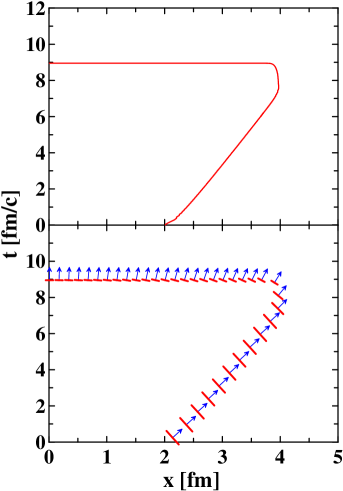
Figure 1: (Color online) Freeze-out hypersurface for hydrodynamic evolution the 1D step-like slab of nuclear matter (see subsect. III.3). Initial conditions for this slab are constructed on the assumption that they are formed by the shock-wave mechanism in head-on collisions of two 1D slabs at $E_{\mbox{\scriptsize lab}}=$ 10 $A$ GeV. The upper panel displays the Cooper–Frye choice for the hypersurface. The lower panel schematically illustrates Milekhin’s choice for the hypersurface. Arrows indicate local 4-velocities on this hypersurface.

Therefore, Milekhin’s method in fact conserves the energy, but to see it one should consider it on a discontinuous hypersurface. The baryon number conservation can be demonstrated in a similar way. The fact that different single-particle distributions (i.e. Cooper–Frye, cut-Jüttner with renormalization, canceling-Jüttner, and even Milekhin’s distributions) provide all the required conservation laws and at the same time produce different particle spectra, cf. Eq. (1) and Refs. Cooper ; Gorenstein84 , only increases ambiguity of freeze-out consequences and indicate the barest necessity for further studies of the freeze-out. Such studies of the freeze-out in a finite 4-volume (a finite space-like layer Csernai05 ) are now in progress.

From the practical point of view, assumption (II) means that we should first run the hydro calculation without any freeze-out and only after that look for a hypersurface, where the freeze-out criterion is met. This hypersurface is determined as if the hydrodynamic system is not affected by the freeze-out. This procedure indeed results in a continuous hypersurface, which could justify assumption (I). The method of “continuous emission” Sinyukov02 offers a more consistent way of performing freeze-out. This method considers a continuous emission of particles from a finite volume, governed by their mean free paths. In this approach the freeze-out process looks like an evaporation (or fragmentation, on account of final-size grid) first from the system surface and then as a volume fragmentation of the system residue. The particle emission from surface layer of the mean-free-path width may hint at a discreetness of the hypersurface arising when this width is shrunk to zero.

In particular, the continuous-emission mechanism implies that dynamics of this evaporation, characterized by its own rate, competes with the hydrodynamic expansion. Therefore, freeze-out front may not reach the places, where, e.g., the energy density reaches the critical value. This is already a consequence of real freeze-out dynamics. Unfortunately, this method is very difficult for the numerical implementation because probability for a particle to leave the hydrodynamic system depends not only on the past but also on the future evolution of this system, since particle emission occurs from time-evolving system.

Assumption (III) is also an approximation to reality. This was the reason why cascading was applied after the hydrodynamic freeze-out in Refs. HS95 ; Bass00 ; Hirano06 ; Nonaka06 . This cascading allowed, in particular, to reproduce a two-slope form of transverse-mass spectra HS95 and a correct value of elliptic flow Teaney01 ; Hirano07 . Inclusion of some inelastic channels in this cascading may be important for proper reproduction of multiplicities, e.g., the $K^{-}$ multiplicity 3FD . However, even this cascading is not enough. A mean-field cascading is really needed. The reasons for this are as follows. First of all, the matter at the freeze-out instant is still dense enough, such that a part of energy is accumulated in collective mean fields. This mean-field energy should be released before calculating observables. In the presently discussed 3FD model 3FD we do this at the freeze-out stage by recalculating thermodynamic quantities in terms the hadronic gas EoS rather than a nontrivial EoS used in the hydro computation.

III Freeze-out in 3FD

The freeze-out scheme adopted in the 3FD model is an attempt to modify and improve the standard freeze-out procedure in certain aspects rather than a final solution of the freeze-out problem. Let us start with criteria of the freeze-out. We formulate these criteria in terms of energy density, which is a universal quantity applicable both at very high energies (instead of temperature) and at low energies (instead of baryon density).

(i) The freeze-out criterion we use is

$$\varepsilon<\varepsilon_{\mbox{\scriptsize frz}},$$ (9)

where

$$\varepsilon=u_{\mu}T^{\mu\nu}u_{\nu}$$ (10)

is the total energy density of all three fluids in the proper reference frame, where the composed matter is at rest. This total energy density is defined in terms of the total energy–momentum tensor

$$T^{\mu\nu}\equiv T^{\mu\nu}_{\mbox{\scriptsize p}}+T^{\mu\nu}_{\mbox{\scriptsize t}}+T^{\mu\nu}_{\mbox{\scriptsize f}}$$ (11)

being the sum over energy–momentum tensors of separate fluids, and the total collective 4-velocity of the matter

$$u^{\mu}=u_{\nu}T^{\mu\nu}/(u_{\lambda}T^{\lambda\nu}u_{\nu}).$$ (12)

Note that definition (12) is, in fact, an equation determining $u^{\mu}$. In general, this $u^{\mu}$ does not coincide with 4-velocities of separate fluids. This definition of the collective 4-velocity is in the spirit of the Landau–Lifshitz approach to viscous relativistic hydrodynamics Land-Lif . Only the formed (to the time instant of consideration) part of the f-fluid is taken into account in $T^{\mu\nu}_{\mbox{\scriptsize f}}$ of Eq. (11). To the end of the freeze-out process all f-fluid turns out to be formed and hence frozen out.

In the present simulations we use the value $\varepsilon_{\mbox{\scriptsize frz}}=0.4$ GeV/fm³ as the critical freeze-out energy density, with the exception of low incident energies $E_{\mbox{\scriptsize lab}}$, for which we use lower values: $\varepsilon_{\mbox{\scriptsize frz}}(2A\mbox{ GeV})=0.3$ GeV/fm³ and $\varepsilon_{\mbox{\scriptsize frz}}(1A\mbox{ GeV})=0.2$ GeV/fm³.

(ii) In order to prevent freeze-out of initial cold nuclei, we apply the additional criterion

$$u_{\mu}\partial^{\mu}\varepsilon<0\quad\mbox{at the system surface},$$ (13)

i.e. at the boarder of matter with vacuum, which coincides with the freeze-out front. In the frame, where the freeze-out front is at rest, $\partial_{t}\varepsilon=0$, condition (13) reduces to ${\bf u}{\bf\nabla}\varepsilon<0$, which demands that collective velocity of the matter is directed outside the system. To meet this condition, we in fact start the freeze-out procedure only at the expansion stage of the collision (see next subsect.).

(iii) A very important feature of our freeze-out procedure is an anti-bubble prescription, preventing formation of bubbles of frozen-out matter inside the dense matter still hydrodynamically evolving. The matter is allowed to be frozen out (provided two above criteria are met) only if
(a) either the matter is located near the boarder with vacuum (this piece of matter gets locally frozen out)
(b) or the maximal value of the total energy density in the system is less than $\varepsilon_{\mbox{\scriptsize frz}}$

$$\max\varepsilon\leq\varepsilon_{\mbox{\scriptsize frz}}$$ (14)

(the whole system gets instantly frozen out).

Criterion (iiib) is convenient for numerical implementations while does not look quite physical. From physical point of view, it would be preferable to change $\max\varepsilon$ to the energy density averaged over the system, $\langle\varepsilon\rangle$. In view of the discussion below, such a substitution will not change the qualitative pattern of the freeze-out, however, can somewhat affect quantitative results at AGS energies.

Before the instant of the global freeze-out, cf. (iiib), above freeze-out criteria can be summarized in terms of dynamic equations

$$\partial_{\mu}J_{\alpha}^{\mu}=\Theta_{\mbox{\scriptsize frz}}J_{\alpha}^{\mu}\partial_{\mu}\Theta_{\mbox{\scriptsize s}},$$ (15)

$$\partial_{\mu}T^{\mu\nu}_{\alpha}=(\mbox{Friction})^{\nu}+\Theta_{\mbox{\scriptsize frz}}T^{\mu\nu}_{\alpha}\partial_{\mu}\Theta_{\mbox{\scriptsize s}},$$ (16)

where $J_{\alpha}^{\mu}$ is the baryon current of the $\alpha$ fluid, $\alpha=$ p, t or f (i.e. projectile, target or fireball), note that $J_{\mbox{\scriptsize f}}^{\mu}\equiv 0$. Here $(\mbox{Friction})^{\nu}$ stands for interaction terms between fluids, the explicit form of which is not important here. $\Theta_{\mbox{\scriptsize s}}$ is a step function at the system surface, which takes into account criterion (iiia). 1-dimensional simulations of the freeze-out (i)-(iiia) show that it results in discontinuity of $\varepsilon$ (and other quantities) at the system surface. This discontinuity is numerically smeared out only to the extent of the finite grid step. Therefore, in analytic equations the step function $\Theta_{\mbox{\scriptsize s}}$ can be represented by a sharp step function

$$\Theta_{\mbox{\scriptsize s}}=\Theta(\varepsilon-\delta)$$ (17)

with $\delta\to+0$. The function

$$\Theta_{\mbox{\scriptsize frz}}=\Theta(\varepsilon_{\mbox{\scriptsize frz}}-\varepsilon^{s})\Theta(-u_{\mu}\partial^{\mu}\varepsilon)$$ (18)

with $\varepsilon^{s}$ being the value of $\varepsilon$ at matter side of the surface discontinuity, takes into account conditions (i) and (ii) of the freeze-out.

Let freeze-out conditions (i) and (ii) be met, i.e. $\Theta_{\mbox{\scriptsize frz}}=1$. To verify that Eqs. (15)–(18) actually correspond to the above described scheme (i)-(iiia), let us consider these equations for the stationary situation in the reference frame, where the freeze-out front is at rest, i.e. $\partial_{t}\Theta_{\mbox{\scriptsize s}}=0$. For the sake of convenience, let us associate the freeze-out front with the $x=0$ plane. Then the only nonzero component of the $\partial_{\mu}\Theta_{\mbox{\scriptsize s}}$ 4-vector is $\partial_{x}\Theta_{\mbox{\scriptsize s}}=-\delta(x)$ (the hydrodynamic matter occupies the $x<0$ semi-space), and Eqs. (15)–(16) take the form

$$\partial_{x}J_{\alpha}^{x} = -J_{\alpha(s)}^{x}\delta(x),$$

$$\partial_{x}T^{x\nu}_{\alpha} = -T^{x\nu}_{\alpha(s)}\delta(x),$$

where symbol $(s)$ in the subscript indicate that the value is taken at the matter side of the freeze-out front. The latter is the effect of $\delta\to+0$ introduced in Eq. (18). We have also omitted friction forces in the r.h.s. of Eq. (16), since they are really unimportant at the freeze-out stage. Integrating above equations over small $\Delta x$ around $x=0$, we arrive at

$$\Delta J_{\alpha}^{x} \equiv J_{\alpha(x>0)}^{x}-J_{\alpha(s)}^{x}=-J_{\alpha(s)}^{x},$$

$$\Delta T^{x\nu}_{\alpha} \equiv T^{x\nu}_{\alpha(x>0)}-T^{x\nu}_{\alpha(s)}=-T^{x\nu}_{\alpha(s)}.$$

Thus, terms $\propto\partial_{\mu}\Theta_{\mbox{\scriptsize s}}$ in the r.h.s. of Eqs. (15) and (16) play role of sinks, which remove matter from hydrodynamic evolution, making the hydrodynamic quantities $J_{\alpha(x>0)}$ and $T_{\alpha(x>0)}$ to be zero after the freeze-out front.

This kind of freeze-out is similar to the model of “continuous emission” proposed in Ref. Sinyukov02 . There the particle emission occurs from a surface layer of the mean-free-path width. In our case the physical pattern is similar, only the mean free path is shrunk to zero.

The above discussion concerns only the first part of the freeze-out procedure, i.e. the application of freeze-out conditions. The second part consists in calculation of spectra of observable particles:

(iv) Milekhin’s method Milekhin , defined on a discontinuous hypersurface was used for calculation of observables, cf. sect. II.

Thus, this freeze-out is similar to evaporation of particles from a free surface of the system followed by explosion of the fluid residue, if criterion (9) is met in the whole finite volume of this residue.

III.1 Physical pattern of the freeze-out

The physical pattern behind this freeze-out resembles the process of expansion of compressed and heated classical fluid into vacuum. Physics of this process is studied both experimentally and theoretically evap76 ; evap82 ; evap92 ; evap99 . Evaporation from free surface of normal (not superheated) fluid is a very slow process. Accordingly, the freeze-out of matter of high density ($\varepsilon>\varepsilon_{\mbox{\scriptsize frz}}$) is suppressed in our model. During expansion the fluid becomes more rarefied, still remaining quite hot. Thus, the fluid becomes superheated at $\varepsilon<\varepsilon_{\mbox{\scriptsize frz}}$. It occurs first at the periphery of the system, which is first affected by the decompression wave. Evaporation from free surface of superheated fluid is already a fast process. Accordingly, the freeze-out is allowed at $\varepsilon<\varepsilon_{\mbox{\scriptsize frz}}$.

Situations are possible, when freeze-out criterion (9) is met in the whole slab near the free surface rather than only at the surface. Such situations are illustrated in Subsects. III.3 and III.4. Here we have a choice either to instantaneously freeze out this whole near-surface slab or to wait until the freeze-out front will gradually traverse this slab (if ever). Making this choice, we rely on results of experiments on evaporation from superheated fluids. It was shown (see, e.g., Ref. evap99 ) that the evaporation front propagates with respect to fluid not faster than with the speed of sound. Precisely this choice is realized in our model by means of condition (iiia) or alternatively by dynamic equations (15) and (16). Thus, the freeze-out front may stay at essentially lower energy densities than $\varepsilon_{\mbox{\scriptsize frz}}$ because supersonic fluid expansion prevents it from reaching the region, where $\varepsilon=\varepsilon_{\mbox{\scriptsize frz}}$.

Physically it implies that a particle is evaporated (”frozen-out”) only if it escapes from the system without collisions. Thus, its mean free path ($\lambda_{\mbox{\scriptsize mfp}}$) should be larger than its path to the free surface (with due account of the future evolution of the fluid). Precisely this criterion is applied in the model of “continuous emission” Sinyukov02 . In our simplified version of the “continuous emission”, $\lambda_{\mbox{\scriptsize mfp}}=0$ in the fluid phase and $\lambda_{\mbox{\scriptsize mfp}}\to\infty$ in the gas phase. Therefore, a particle can escape only from the free surface, which cannot move inward the system faster than with the speed of sound evap99 .

The only exception from this rule we do at the final stage of the freeze-out. As it was observed in experiments with classical fluids (see, e.g., Ref. evap82 ), a fluid transforms into gas by explosion, if it is strongly superheated all over its volume. Therefore, at the final stage of the freeze-out, when criterion (9) is met in the whole volume of the fluid residue, we assume that the whole residue becomes frozen out simultaneously (condition (iiib)).

Of course, criterion (9) is not universal. In particular, it is not applicable to the cold nuclear matter, which has $\varepsilon\approx$ 0.15 GeV/fm³ in its ground state. Additional condition (13), preserving the cold nuclear matted from being frozen out, is directly connected with this fact. We hope that criterion (9) is good enough for a restricted domain of the phase diagram, where freeze-out of hot nuclear matter really occurs.

In order to further clarify our freeze-out scheme it is useful to consider the way it was implemented in the numerical scheme.

III.2 Numerical implementation of the freeze-out

The numeric scheme of the 3FD code is based on the modified particle-in-cell method Roshal81 ; FCT-PIC , which is an extension of the scheme first applied in Los-Alamos Harlow76 . In the particle-in-cell method each time step of the computation consists of three stages: (I) Eulerian stage, (II) Lagrangian stage, and (III) transformation from the frame of computation to the local rest frame of fluids in order to calculate thermodynamic quantities and flow velocities (as applied to the freeze-out, it is described in point (c) of this subsect.).

The transfer of energy–momentum due to pressure gradients, friction between fluids and production of the fireball fluid is computed on the spatially fixed grid (so called Eulerian stage of the scheme). The convective transfer of the baryonic charge, energy and momentum is performed at the Lagrangian stage of the scheme. At this stage the matter is represented by an ensemble of Lagrangian particles which accumulate all the energy, momentum and baryon charge of the system. At the time step (let it be “1”), when the freeze-out has not started yet, the total energy–momentum ($P^{\mu}_{\mbox{\scriptsize tot}}$) and baryon charge ($B_{\mbox{\scriptsize tot}}$) are presented by sums over these particles

$$P^{\mu}_{\mbox{\scriptsize tot}} = \sum_{i\alpha}\Delta P^{\mu}_{i\alpha}(t_{1})=\sum_{i\alpha}{\Delta V_{i\alpha}(t_{1})}\ T^{\mu 0}_{(i\alpha)}(t_{1}),$$ (19)

$$B_{\mbox{\scriptsize tot}} = \sum_{i\alpha}\Delta B_{i\alpha}(t_{1})=\sum_{i\alpha}{\Delta V_{i\alpha}(t_{1})}\ J^{0}_{(i\alpha)}(t_{1}),$$ (20)

where $\Delta P^{\mu}_{i\alpha}(t_{1})$ and $\Delta B_{i\alpha}(t_{1})$ are respectively the energy–momentum and baryon charge of an $i$th particle belonging to the $\alpha$-fluid. These sums run over both formed and still unformed particles of the f-fluid. In fact, baryon charges of all particles belonging to a baryon-rich fluid are taken to be constant and equal, $\Delta B_{ip}(t)=b_{p}$ and $\Delta B_{it}(t)=b_{t}$ ($b_{p}=b_{t}$ if nuclei are identical), while for the f-fluid $\Delta B_{if}(t)=0$. Each Lagrangian particle is also characterized by a volume $\Delta V_{i\alpha}(t_{1})$. Therefore, the above quantities of the particle are expressed in terms of respective densities $T^{\mu 0}_{(i\alpha)}$ and $J^{0}_{(i\alpha)}$, as it is indicated in Eqs. (19) and (20). Simulation is performed in the frame of equal velocities of colliding nuclei. Hence, all the quantities in Eqs. (19) and (20) are related to this frame. Eqs. (19) and (20) imply that all the matter participates in dynamical evolution before the freeze-out starts:

$$P^{\mu}_{\mbox{\scriptsize dyn}}(t_{1})=P^{\mu}_{\mbox{\scriptsize tot}},\quad\quad B_{\mbox{\scriptsize dyn}}(t_{1})=B_{\mbox{\scriptsize tot}}.$$ (21)

Here $P^{\mu}_{\mbox{\scriptsize dyn}}$ and $B_{\mbox{\scriptsize dyn}}$ are respectively total energy–momentum and baryon charge participating in dynamical evolution. We avoid term “hydrodynamic evolution” because a part of the f-fluid may be still unformed.

In the present scheme the Lagrangian particle has a profile function of the form and size of the grid cell with uniform distribution of densities. Therefore, in 3D simulations a single Lagrangian particle contributes to 8 cells on the grid, with which it overlaps. These spatially extended particles make the scheme smoother and hence more stable. In Refs. 3FD ; MRS91 this numerical scheme is described in more detail.

(a) To roughly meet condition (ii), the freeze-out procedure is started only at the expansion stage of the collision, i.e. after the time interval required for nuclei to traverse each other, provided they keep their initial velocities. In the c.m. frame of two identical nuclei this time delay is $\Delta t_{\mbox{\scriptsize frz}}=D_{A}/(\gamma_{\mbox{\scriptsize cm}}v_{\mbox{\scriptsize cm}})$, where $D_{A}/\gamma_{\mbox{\scriptsize cm}}$ is the Lorentz contracted diameter of the nucleus, $\gamma_{\mbox{\scriptsize cm}}$ and $v_{\mbox{\scriptsize cm}}$ are the $\gamma$ factor and the initial velocity of the nucleus in the c.m. frame, respectively.

(b) The freeze-out criterion (9) is checked at the Lagrangian stage of each time step (let it be $n$th step). In the f-fluid only those particles are considered which have been formed to the time instant $t_{n}$. For each Lagrangian particle it is checked in all cells, which overlap with this considered particle, i.e. in 8 cells.

If the freeze-out criterion is met in all these 8 cells and if at least one of these cells is “empty” (i.e. contains no centers of any Lagrangian particles), then this considered Lagrangian particle is counted as frozen out. This is realization of condition (iiia). This frozen-out Lagrangian particle is removed from further hydrodynamic evolution. By doing this we remove respective portions from sums (19) and (20):

$$P^{\mu}_{\mbox{\scriptsize dyn}}(t_{n}) = P^{\mu}_{\mbox{\scriptsize dyn}}(t_{n-1})-\sum_{i\alpha\mbox{\scriptsize frozen out at }t_{n}}\Delta P^{\mu}_{i\alpha}(t_{n}),$$ (22)

$$B_{\mbox{\scriptsize dyn}}(t_{n}) = B_{\mbox{\scriptsize dyn}}(t_{n-1})-\sum_{i\alpha\mbox{\scriptsize frozen out at }t_{n}}\Delta B_{i\alpha}(t_{n}).$$ (23)

Only parts $P^{\mu}_{\mbox{\scriptsize dyn}}(t_{n})$ and $B_{\mbox{\scriptsize dyn}}(t_{n})$ are kept in further dynamic evolution, unlike the conventional Cooper–Frye method. It is important to mention that had we kept this frozen-out particle in the dynamic evolution, its energy–momentum content would be changed at later time steps, and hence a part of its energy–momentum would be gained by other particles. Then we would face problems with the energy–momentum conservation, if we wanted to use the $\Delta P^{\mu}_{i\alpha}$ quantity at the instant of its freeze-out for calculation of observable spectra.

If the freeze-out criterion is met in all cells of the system, all Lagrangian particles are counted as frozen out at this time step, as it is required by condition (iiib). This is the end of the freeze-out process.

(c) When the freeze-out process is over, i.e. $P^{\mu}_{\mbox{\scriptsize dyn}}=0$ and $B_{\mbox{\scriptsize dyn}}=0$, we are left with ensemble of frozen-out Lagrangian particles which precisely obeys conservation laws:

$$P^{\mu}_{\mbox{\scriptsize tot}} = \sum_{i\alpha}\Delta P^{\mu}_{i\alpha}(t_{i\alpha\mbox{\scriptsize frozen-out}}),$$ (24)

$$B_{\mbox{\scriptsize tot}} = \sum_{i\alpha}\Delta B_{i\alpha}(t_{i\alpha\mbox{\scriptsize frozen-out}}).$$ (25)

Here the summation runs over frozen-out (at different time instants $t_{i\alpha\mbox{\scriptsize frozen-out}}$) particles, unlike sums (19) and (20), where this summation is associated with a fixed time instant. These frozen-out particles are precisely those droplets mentioned in Eq. (3).

A frozen-out $i\alpha$-particle is still characterized by five hydrodynamic quantities, $J^{0}_{i\alpha}$ and $T^{\mu 0}_{i\alpha}$, and volume $\Delta V_{i\alpha}$, all these in the reference frame of computation. For the calculation of spectra we need distribution function formulated in terms of thermodynamic quantities: temperature ($T^{i\alpha}$), baryon ($\mu_{b}^{i\alpha}$) and strange ($\mu_{s}^{i\alpha}$) chemical potentials, and hydrodynamic 4-velocity ($u^{\mu}_{i\alpha}$), cf. Eqs. (1) and (2). In fact, this recalculation of the hydrodynamic quantities into thermodynamic ones is performed at each time step of the scheme based on the nongas EoS (involving some mean fields) accepted in the calculation. This EoS is not suitable for calculation of the spectrum of observable particles. First we should release the energy stored in mean fields. To do this, we calculate $T^{i\alpha\mbox{\scriptsize(gas)}}$, $\mu_{b}^{i\alpha\mbox{\scriptsize(gas)}}$, $\mu_{s}^{i\alpha\mbox{\scriptsize(gas)}}$ and $u^{\mu}_{i\alpha\mbox{\scriptsize(gas)}}$ based on the hadronic gas EoS and proceeding from conservations of total energy–momentum, baryon and strange charges in the frozen-out particle.

(d) At this stage we are still free to choose either Cooper–Frye or Milekhin’s scheme to calculate observables, as it was argued in Eqs. (3)–(8). We use Milekhin’s method Milekhin , defined on a discontinuous hypersurface consisting of tiny fragments coinciding with volumes of frozen-out Lagrangian particles $\Delta V_{i\alpha}$. The observable spectrum of hadrons is calculated as follows

$$E\frac{dN}{d^{3}p}=\sum_{i\alpha}V_{i\alpha}^{\mbox{\scriptsize(proper)}}p_{\mu}u^{\mu}_{i\alpha\mbox{\scriptsize(gas)}}f_{i\alpha\mbox{\scriptsize(gas)}}(p)$$ (26)

where $V_{i\alpha}^{\mbox{\scriptsize(proper)}}$ is the volume of the $i\alpha$-particle in its rest frame, the sum runs over all frozen-out particles of all fluids, $f_{i\alpha\mbox{\scriptsize(gas)}}(p)$ is the equilibrium distribution function defined already in terms of local gas thermodynamic ($T^{i\alpha\mbox{\scriptsize(gas)}}$, $\mu_{b}^{i\alpha\mbox{\scriptsize(gas)}}$ and $\mu_{s}^{i\alpha\mbox{\scriptsize(gas)}}$) and hydrodynamic ($u^{\mu}_{i\alpha\mbox{\scriptsize(gas)}}$) quantities, cf. Eqs. (1) and (2).

In this prescription the baryon number and energy-momentum are precisely conserved by construction. It is worthwhile to mention that both the Cooper–Frye and Milekhin methods possess the same main problem: they both do not reject contributions of frozen-out hadrons returning into the hydrodynamic phase and do this to precisely the same extent, see Appendix A. In particular, in our calculation this problem probably reveals itself in the failure of reproduction of the pion directed flow 3FD ; 3FDflow . The advantage of Milekhin’s method is just practical: with the exception of the pion directed flow it quite successfully works in the 3FD model. The canceling-Jüttner recipe Csernai04 overcomes the returning-hadrons problem of the above methods. It would be of interest to apply it in the 3FD model.

III.3 One-dimensional simulations

In order to clarify physics described by Eqs. (15)–(18) let us consider 1D simulations based on them. In Fig. 2 decays of step-like slabs of nuclear matter are presented. These simulations have been performed till the time instant of the global freeze-out, i.e. when criterion (iiib) is met. The same EoS as that used in 3D simulations 3FD ; 3FDflow ; 3FDpt is accepted in the present calculations. First of all, we see that the freeze-out front is really step-like. It is smeared only over two cells (independently of their size) due to numeric scheme. Note also that for this step-like initial geometry the supersonic flow of matter ($v_{x}>c_{s}$, where $c_{s}$ is the speed of sound) always occurs beyond the initial boundary of the slab, while the flow within the initial boundary is always subsonic ($v_{x}<c_{s}$). This is important for understanding results displayed in Fig. 2.

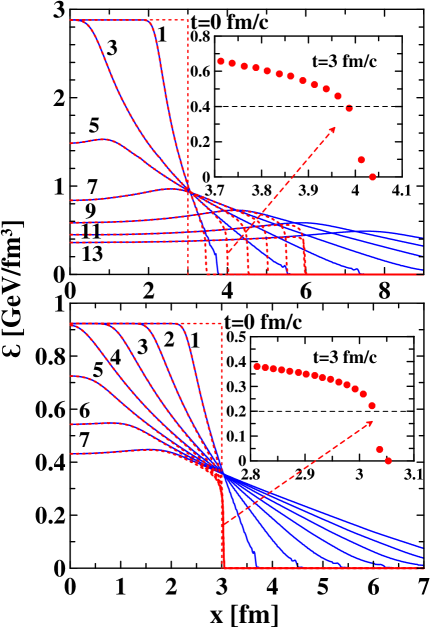
Figure 2: (Color online) Evolution of the energy density during the decay of the 1D step-like slab of nuclear matter. Solid lines display calculations without freeze-out, while dashed lines, with freeze-out. Initial conditions for these slabs are constructed on the assumption that they are formed by the shock-wave mechanism in head-on collisions of two 1D slabs at $E_{\mbox{\scriptsize lab}}=$ 10 $A$ GeV for upper panel and $E_{\mbox{\scriptsize lab}}=$ 2 $A$ GeV for lower panel. Subpanels show zoomed regions of the freeze-out front at the fixed time instant $t=$ 3 fm/c in terms of the energy density in separate cells (displayed by dots).

There are three important velocities in this problem: the hydrodynamic velocity of the matter ($v_{x}$) at the position, where the freeze-out front occurs, the speed of sound $c_{s}$, and the velocity $v_{\varepsilon}$ of transfer of the constant value of $\varepsilon=0.4$ GeV/fm³:

$$\varepsilon(v_{\varepsilon}t+\mbox{const},t)=0.4\ \mbox{GeV/fm}^{3}.$$ (27)

In fact, Eq. (27) is the equation for the hydrodynamic characteristic curve related to the 0.4 GeV/fm³ value of the energy density. The freeze-out front, as defined by Eq. (15) and (16), cannot propagate in the fluid medium faster than with the local speed of sound, like any perturbation in the hydrodynamics.

Different dynamic patterns of the freeze-out fronts displayed in two panels of Fig. 2 are associated with different relations between above three velocities. In the upper case of $\varepsilon_{0}\simeq 3$ GeV/fm³ we have $v_{\varepsilon}>0$. Hence, the point, where the freeze-out criterion (18) starts to be met, is transferred farther and farther from the initial system boundary, hence the system expands. In this region the flow is supersonic: $v_{x}>c_{s}$. At the same time, the matter velocity with respect to the characteristic velocity is $(v_{x}-v_{\varepsilon})/(1-v_{x}v_{\varepsilon})\leq c_{s}$, i.e. it is less than the speed of sound. Therefore, the fluid flow does not carry the freeze-out front away from the point of $\varepsilon=0.4$ GeV/fm³, where the freeze-out criterion (18) is met. The freeze-out front stays at this position, see the zoomed subpanel in the top panel of Fig. 2. Since the matter within this freeze-out front is distributed over the range of $0<\varepsilon<0.4$ GeV/fm³, an average value for the actual energy density of the frozen-out matter (let us denote it as $\varepsilon_{\mbox{\scriptsize out}}$) is approximately half of the freeze-out jump, i.e. $\varepsilon_{\mbox{\scriptsize out}}\approx\varepsilon_{\mbox{\scriptsize frz}}/2=0.2$ GeV/fm³ in this case, see Fig. 3.

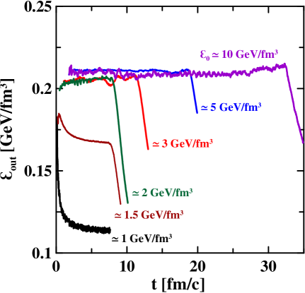
Figure 3: (Color online) Instant values of actual energy density of the frozen-out matter for decays of nuclear-matter slabs with various initial conditions (labeled by initial energy densities $\varepsilon_{0}$). Initial conditions are constructed on the assumption of the shock-wave mechanism in head-on collisions of two slabs at $E_{\mbox{\scriptsize lab}}=$ 2, 4, 6, 10, 20 and 40 $A$ GeV (from bottom left to top right). The time evolution is displayed till the time instant of the global freeze-out (iiib).

In the bottom panel of Fig. 2, i.e. $\varepsilon_{0}\simeq 1$ GeV/fm³, we have $v_{\varepsilon}<0$. Here, the point, where freeze-out criterion (18) starts to be met, cannot be reached by the freeze-out front. Indeed, the freeze-out front is first formed beyond the initial boundary of the slab, i.e. in the region of the supersonic flow of the matter. Since it cannot be faster than the sound, it cannot overcome the “supersonic barrier” in the back direction in order to reach the $\varepsilon=0.4$ GeV/fm³ point. It stays at the position of the “supersonic barrier” and does not move. Therefore, the decaying and freezing-out system does not expand. Moreover, the front stays at the position of low energy density, $\varepsilon\simeq 0.2$ GeV/fm³, see the zoomed subpanel in the bottom panel of Fig. 2. Therefore, the actual energy density of the frozen-out matter turns out to be lower than $\varepsilon_{\mbox{\scriptsize frz}}/2$ (as in above case), i.e. $\varepsilon_{\mbox{\scriptsize out}}\approx(0.2$ GeV/fm${}^{3})/2=0.1$ GeV/fm³, see Fig. 3.

In Fig. 3 we see that $\varepsilon_{\mbox{\scriptsize out}}$ remains practically constant during the major period of the freeze-out. The steep fall of $\varepsilon_{\mbox{\scriptsize out}}$ just before the global freeze-out occurs because the velocity $v_{\varepsilon}$ on the characteristic curve (27) changes its sign. Then the point, where $\varepsilon=0.4$ GeV/fm³ is achieved, starts rapidly move inwards the system, and hence the freeze-out front remains at lower energy density.

Thus, we see that the freeze-out is not inseparably linked with the freeze-out energy density $\varepsilon_{\mbox{\scriptsize frz}}$ but can occur at lower energy densities due to dynamical reasons. At low initial energy densities the freeze-out front stays at lower energy densities than $\varepsilon_{\mbox{\scriptsize frz}}$ and hence the actual energy density of the frozen-out matter $\varepsilon_{\mbox{\scriptsize out}}$ turns out to be lower than $\varepsilon_{\mbox{\scriptsize frz}}/2$, see Fig. 3. With the initial energy density rising, the $\varepsilon_{\mbox{\scriptsize out}}$ quantity grows and gradually reaches the $\varepsilon_{\mbox{\scriptsize frz}}/2$ value and than approximately saturates.

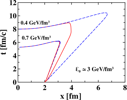
Figure 4: (Color online) Characteristic curves for hydrodynamic evolution the 1D step-like slab with initial conditions corresponding to the upper panel of Fig. 2. Solid lines display characteristic curves, corresponding to $\varepsilon=0.4$ and 0.7 GeV/fm³, calculated with local freeze-out (iiia) but without global freeze-out (iiib). Dashed lines correspond to the calculation without freeze-out.

A standard procedure of performing freeze-out, which is applied in the major part of hydrodynamic calculations now, proceeds in the following way. The hydro calculation runs absolutely unrestricted. The freeze-out hypersurface is determined by analyzing the resulting 4-dimensional field of hydrodynamic quantities on the condition of the freeze-out criterion met. In our case this would be the characteristic curve of $\varepsilon=0.4$ GeV/fm³ calculated without freeze-out, displayed in Fig. 4.

In the 3FD model, the freeze-out criterion is checked continuously during the simulation. If some parts of the hydro system meet all criteria ((i), (ii), and either (iiia) or (iiib)), they decouple from the hydro calculation. The frozen-out matter escapes from the system, removing all the energy and momentum accumulated in it, cf. Eq. (3). Therefore, it produces no recoil to the rest of still hydrodynamic system. The removal of the matter affects the system evolution. This influence is illustrated in Fig. 4. The $\varepsilon=0.4$ GeV/fm³ characteristic curves calculated with and without freeze-out turn out to be different. At the same time the $\varepsilon=0.7$ GeV/fm³ characteristic curves, which lie quite deep inside the system, remain unaffected by the freeze-out. The freeze-out hypersurface (i.e. curve in 1+1 dimensions) for this case is presented in Fig. 1. It differs from the corresponding characteristic curve because of the global freeze-out which occurs at time instant $t\simeq$ 9 fm/c.

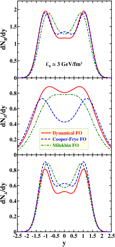
Figure 5: (Color online) Rapidity distributions of baryons (upper panel), thermal pions (middle panel) and $\Delta$-isobars (lower panel) calculated within three models of freeze-out: the model of dynamical freeze-out [Dynamical FO], [see Eqs. (9)–(26)], Cooper–Frye freeze-out on characteristic curve (27) [Cooper–Frye FO], and Milekhin freeze-out on characteristic curve (27) [Milekhin FO].

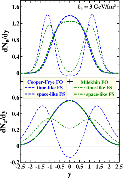
Figure 6: (Color online) Partial contributions to rapidity spectra of baryons (upper panel) and thermal pions (lower panel) from space-like and time-like parts of the freeze-out surface. Spectra are calculated within two models of freeze-out: Cooper–Frye freeze-out on characteristic curve (27) [Cooper–Frye FO], and Milekhin freeze-out on the same characteristic curve [Milekhin FO].

It is of interest to compare particle spectra predicted by different models for freeze-out. In Fig. 5 rapidity distributions of various hadrons are demonstrated for three different prescriptions of the freeze-out: the above-described model of dynamical freeze-out (Dynamical FO) [see Eqs. (9)–(26)], Cooper–Frye freeze-out on characteristic curve (27) [Cooper–Frye FO], and Milekhin freeze-out on characteristic curve (27) [Milekhin FO]. These spectra were calculated within 1D hydrodynamic expansion of the slab of initial width of 4 fm and initial energy density $\varepsilon_{0}=3$ GeV/fm³. Initial conditions for this slab are constructed on the assumption that it is formed formed by the shock-wave mechanism in head-on collision of two 1D slabs at $E_{\mbox{\scriptsize lab}}\simeq$ 10 $A$ GeV. Only nucleons, deltas and pions are included in the EoS used in this calculation. Displayed rapidity distributions are normalized to unit aria transverse to the direction ($x$) of longitudinal expansion. Freeze-out surfaces for these three models of freeze-out are displayed in Fig. 1 for Dynamical FO and Fig. 4 (dashed curve for $\varepsilon=0.4\ \mbox{GeV/fm}^{3}$) for Cooper–Frye FO and Milekhin FO.

It is difficult to directly compare the Dynamical FO and Cooper–Frye FO, since the Dynamical FO surface is inappropriate for the Cooper–Frye FO and vise versa. This is because the Dynamical FO requires the hydrodynamics to be modified by removing the frozen-out matter, while the Cooper–Frye FO needs the hydro calculation to be run absolutely unrestricted. This is the reason why we consider the Milekhin FO, which takes place precisely on the same characteristic curve (27) as the Cooper–Frye FO. In particular, this is the reason why we compare only two models in Fig. 6.

As seen from Fig. 5, baryon rapidity distributions are quite close to each other within different freeze-out models. The Dynamical-FO and Cooper–Frye-FO are even strikingly close. Apparently, this occurs because they are confined by the baryon number conservation. This is not the case for thermal pions (i.e. without contribution of $\Delta$ decays). Difference between their distributions within different models is quite spectacular.

As it is seen from Fig. 6, this difference mainly originates from contributions from the time-like parts of the freeze-out surface, i.e. from those parts, where the the Cooper–Frye normal vector $n^{\mu}_{CF}$ is space-like: $n_{CF}\cdot n_{CF}<0$. Difference between Cooper–Frye and Milekhin recipes is most strongly pronounced in this case. Note that the Cooper–Frye FO even reveals its generic deficiency—its ”time-like” spectrum becomes negative at midrapidity. Physically it means that the midrapidity region is most abundantly populated by particles which have to be returned to the hydro phase. At the same time, contributions from the space-like parts of the surface, where $n_{CF}\cdot n_{CF}>0$, are quite similar within Cooper–Frye FO and Milekhin FO. Small diference between the Cooper–Frye normal time-like vector $n^{\mu}_{CF}$ and and the hydrodynamic 4-velocity results is tiny difference in ”time-like” spectra.

Thus, spectra of newly produced particles are quite different in different models of freeze-out. At the same time, the numerical baryon-number and energy conservation is better than 1% in all considered models. We still face the problem: which of these models is physically true. Unfortunately, above-mentioned experiments on expansion of compressed and heated classical fluid into vacuum evap76 ; evap82 ; evap92 ; evap99 cannot answer this question. As we have seen, particle number conservation (baryon number, in Fig. 5) makes these models fairly close to each other. We would like only to mention that the dynamical FO model naturally explains 3FDpt the incident energy behavior of inverse-slope parameters of transverse-mass spectra observed in experiment. However, this is not a physical justification of this model. The question still remains open.

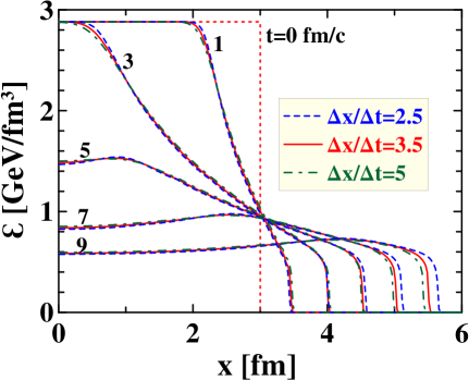
Figure 7: (Color online) The same as in Fig. 2 (top panel) but for different values of $\Delta x/\Delta t$. Only results with freeze-out are displayed.

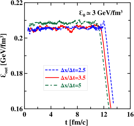
Figure 8: (Color online) The same as in Fig. 3 (bottom panel) but for different values of $\Delta x/\Delta t$.

Results of the above reported 1D simulations are stable with respect to the numeric procedure Roshal81 . They are quite insensitive to the size of the cell. The freeze-out front is smeared only over two cells independently of their size and hence indeed is step-like in continuum limit. Dependence on the most important numeric parameter—the ratio of the space-grid step to the time step $\Delta x/\Delta t$—is displayed in Figs. 7 and 8. To reduce numerical diffusion, this ratio should be taken optimal. As it was found in 1-dimensional simulations of exactly solvable problems FCT-PIC , the optimal range of this ratio is $2.5<\Delta x/\Delta t<5$ with the preferable $\Delta x/\Delta t\simeq 3.5$, minimizing the numerical diffusion. As seen, within this range $2.5<\Delta x/\Delta t<5$ the results are really stable.

III.4 3D simulations

Condition (i) (or Eq. (18)) ensures only that the actual freeze-out energy density, at which the freeze-out actually occurs, is less than $\varepsilon_{\mbox{\scriptsize frz}}$.

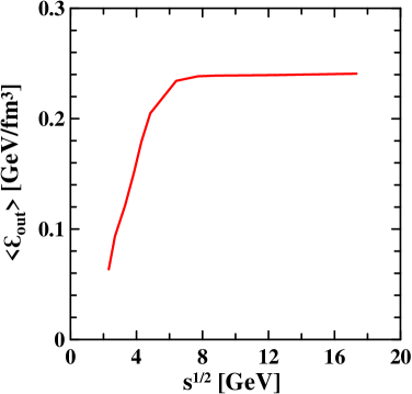
Figure 9: (Color online) Actual average freeze-out energy density in central ($b=0$) Pb+Pb collisions as a function of invariant incident energy.

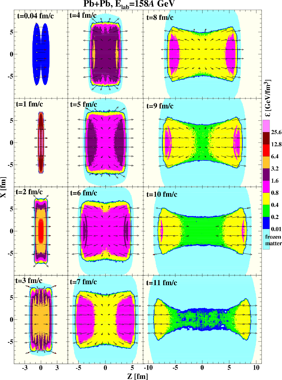
Figure 10: (Color online) Time evolution (in the $xz$ plane of the center-of-mass frame) of the total energy density (cf. Eq. (10)) in the central Pb+Pb collision at $E_{\mbox{\scriptsize lab}}=$ 158$A$ GeV. The light-colored outer hallo corresponds to the simulation without freeze-out and thus indicates the matter which has already been frozen out to the time instant $t$. Arrows indicate velocities of baryon-rich fluids: open arrows for the projectile-like fluid and filled arrows for the target-like fluid.

Therefore, $\varepsilon_{\mbox{\scriptsize frz}}$ can be called a ”trigger” value of the freeze-out energy density. As it has been demonstrated in the previous subsection, a natural value of this actual freeze-out energy density is $\varepsilon_{\mbox{\scriptsize out}}\approx\varepsilon^{s}/2$, i.e. at the middle of the fall from $\varepsilon^{s}$ to zero. To find out the actual value of $\varepsilon_{\mbox{\scriptsize out}}$, we have to analyze results of a particular simulation. In our previous paper 3FD we have performed only a rough analysis of this kind. This is why in the main text of Ref. 3FD we mentioned the value of approximately 0.2 GeV/fm³ for $\varepsilon_{\mbox{\scriptsize out}}$ and in the appendix explained how the freeze-out actually proceeded. Results of more comprehensive analysis for central ($b=0$) Pb+Pb collisions are presented in Fig. 9, which shows the $\varepsilon_{\mbox{\scriptsize out}}$ value averaged over space–time evolution of the collision: $\langle\varepsilon_{\mbox{\scriptsize out}}\rangle$. As seen, $\langle\varepsilon_{\mbox{\scriptsize out}}\rangle$ reveals saturation at the SPS energies. This happens in spite of the fact that our freeze-out condition involves only a single constant parameter $\varepsilon_{\mbox{\scriptsize frz}}=0.4$ GeV/fm³, with the exception of low incident energies, for which we use lower values: $\varepsilon_{\mbox{\scriptsize frz}}(2A\mbox{ GeV})=0.3$ GeV/fm³ and $\varepsilon_{\mbox{\scriptsize frz}}(1A\mbox{ GeV})=0.2$ GeV/fm³.

The ”step-like” behavior of $\langle\varepsilon_{\mbox{\scriptsize out}}\rangle$ is a consequence of the freeze-out dynamics which has already been illustrated in Fig. 3. At low (AGS) incident energies, the energy density achieved at the border with vacuum, $\varepsilon^{s}$, is lower than $\varepsilon_{\mbox{\scriptsize frz}}$. The surface freeze-out stays at this lower energy density up to the global freeze-out because the freeze-out front cannot overcome the supersonic barrier in the expanding matter, cf. the lower panel of Fig. 2. At these low energies, the value $\langle\varepsilon_{\mbox{\scriptsize out}}\rangle$ turns out to be low sensitive to the freeze-out parameter $\varepsilon_{\mbox{\scriptsize frz}}$. Only the global freeze-out (iiib) of the system remnant, which also contributes to $\langle\varepsilon_{\mbox{\scriptsize out}}\rangle$, produces weak sensitivity to $\varepsilon_{\mbox{\scriptsize frz}}$. The values $\varepsilon_{\mbox{\scriptsize frz}}(2A\mbox{ GeV})=0.3$ GeV/fm³ and $\varepsilon_{\mbox{\scriptsize frz}}(1A\mbox{ GeV})=0.2$ GeV/fm³ were precisely chosen in order to reduce contribution of the global freeze-out to $\langle\varepsilon_{\mbox{\scriptsize out}}\rangle$.

With the incident energy rise the energy density achieved at the border with vacuum gradually reaches the value of $\varepsilon_{\mbox{\scriptsize frz}}$ and then even overshoot it. If the overshoot happens, the system first expands without freeze-out. The freeze-out starts only when $\varepsilon^{s}$ drops to the value of $\varepsilon_{\mbox{\scriptsize frz}}$. Then the surface freeze-out occurs really at the value $\varepsilon^{s}\approx\varepsilon_{\mbox{\scriptsize frz}}$ and thus the actual freeze-out energy density saturates at the value $\langle\varepsilon_{\mbox{\scriptsize out}}\rangle\approx\varepsilon_{\mbox{\scriptsize frz}}/2$.

In Fig. 10 the time evolution of the total energy density (cf. Eq. (10)) in the central Pb+Pb collision at $E_{\mbox{\scriptsize lab}}=$ 158$A$ GeV is displayed. The light-colored outer hallo corresponds to the simulation without freeze-out and thus indicates the matter which has already been frozen out to the time instant $t$. First of all we see that already in the beginning of expansion stage ($t=2$ fm/c) the baryon-rich fluids are mutually stopped and unified to a good extent, since their hydrodynamic velocities almost coincide: arrows, originating from the same point, are almost equal if not merged. This is not the case for the baryon-free fluid, since its formation lasts till approximately $t=4$ fm/c (see Fig. 18 in Ref. 3FD ). At the late stage of the expansion ($t\mathrel{\hbox to0.0pt{ \lower 4.0pt\hbox{\hskip-3.0pt$\sim$}\hss}\raise 1.0pt\hbox{$>$}}10$ fm/c) the baryon-rich and baryon-free fluids become even spatially separated: The middle region of the system, containing no arrows, is solely populated by the baryon-free fluid, and hence the baryon-rich matter falls into two disconnected pieces. Thus, at the late stage of the evolution the system effectively consists of three “fireballs” (two baryon-rich and one baryon-free). This is in contrast to the assumption of the statistical model (Andronic06 ; Cleymans06 ; Randrup06 ; Dumitru06 ), where a single uniform “fireball” is considered. The baryon-free “fireball” becomes frozen out first: the displayed time instant $t=11$ fm/c is almost the last, when this “fireball” still hydrodynamically evolves. Evolution of the two baryon-rich “fireballs” till the complete freeze-out is rather long, till $t\approx 20$ fm/c. This spatial separation of “fireballs” happens only at high incident energies $E_{\mbox{\scriptsize lab}}>$ 40$A$ GeV.

The freeze-out in the longitudinal direction proceeds accordingly to the 1D pattern of Fig. 2 (upper panel). In the transverse direction the freeze-out front moves inwards the system. This a combined effect of fast longitudinal expansion and comparatively slow transverse motion of the system. This effect actually results in the “two-fireballs” structure at the latest stage.

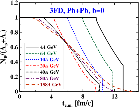
Figure 11: (Color online) Time evolution (in the center-of-mass frame) of the non-frozen-out baryon number (normalized to the total baryon number of the system $A_{p}+A_{t}$) in central Pb+Pb collisions at various incident energies.

The occurrence of two spatially separated “fireballs” at the latest stage of the collision is the reason why the global freeze-out, cf. (iiib), does not occur in this system. At low (AGS) incident energies, the surface freeze-out, actually occurring at lower than $\varepsilon_{\mbox{\scriptsize frz}}$ densities, takes place only as long as the energy density in the center of expanding system exceeds $\varepsilon_{\mbox{\scriptsize frz}}$. When this center density drops below $\varepsilon_{\mbox{\scriptsize frz}}$, the rest of the system instantly gets frozen out, as it is illustrated in Fig. 11 at the example of time evolution the baryon number still involved in the hydrodynamic phase. The abrupt fall of a curve corresponds to the global freeze-out. In fact, only this global freeze-out stage depends on the freeze-out parameter $\varepsilon_{\mbox{\scriptsize frz}}$ at low incident energies. With the incident energy rise this instantly frozen-out remnant becomes smaller and smaller until it completely disappears above $40A$ GeV energy. This happens because outer freeze-out fronts stay already at the $\varepsilon_{\mbox{\scriptsize frz}}$ density, therefore the maximum volume density can be only higher than $\varepsilon_{\mbox{\scriptsize frz}}$. At the same time the inner freeze-out fronts overtake these two baryon-rich “fireballs” from behind and result in gradual surface freeze-out of them without any remnant, where criterion (iiib) can work.

IV Conclusions

The described method of freeze-out can be called dynamical, since the freeze-out process here is integrated into fluid dynamics through hydrodynamic equations (15)–(18). The freeze-out front is not defined just “geometrically” on the condition of the freeze-out criterion met but rather is a subject the fluid evolution. It competes with the fluid flow and not always reaches the place where the freeze-out criterion is met.

This kind of freeze-out is similar to the model of “continuous emission” proposed in Ref. Sinyukov02 . There the particle emission occurs from a surface layer of the mean-free-path width. In our case the physical pattern is similar, only the mean free path is shrunk to zero. In particular, the fact that the freeze-out sometimes occurs at lower energy densities than that prescribed by the freeze-out criterion can be associated with the dependence on the future evolution of the fluid system in the model of “continuous emission”. In that model the particle emission occurs from interior of the time-evolving system. Therefore, if the emitted particle is able to leave the system or not depends on the expansion rate of the system. Similar situations happen in our model. Sometimes the freeze-out criterion is met too deep inside the system such that rapid expansion of the system prevents the freeze-out front from reaching this place.

We argue that the original Milekhin’s method Milekhin of calculation of observable particle spectra is energy conserving, as well as the Cooper–Frye recipe Cooper , provided it is considered on a discontinuous hypersurface, i.e. that consisting of tiny (infinitely small in continuum limit) fragments with normal vectors coinciding with the local hydrodynamic 4-velocity. Moreover, we argue that Milekhin’s approach on a discontinuous hypersurface is natural for the Lagrangian formulation of hydrodynamics. There are no principal objections against using such a fragmented hypersurface instead of the continuous one like in the Cooper–Frye method. Discreetness of particle emission may hint at discontinuous character of the freeze-out hypersurface.

Systematic studies based on hydrodynamic models indicated that there are two distinct freeze-out points (see, e.g., Shuryak99 ; Heinz99 ): chemical and thermal ones. Contrary to these studies we do not need two distinct freeze-out points. Multiplicities and spectra are simultaneously and quite satisfactorily reproduced with the single freeze-out described above 3FD . Of course, we could somewhat refine reproduction of experimental data by introducing two distinct freeze-out points. However, introduction of an additional fitting parameter would be too high price for such a slight improvement.

Appendix A Problem of frozen-out hadrons returning into hydrodynamic phase

When frozen-out matter coexists with still hydrodynamically evolving fluid, both the conventional Cooper–Frye recipe Cooper and the model presented here suffer from a problem of frozen-out particles returning to the hydro phase. For the Cooper–Frye method this problem was discussed in a number of papers Bugaev96 ; Neumann97 ; Csernai97 ; Bugaev99 ; Csernai04 . Here we would like to demonstrated that precisely the same (and precisely to the same extent) problem exists for the freeze-out model discussed in this paper.

Let the fluid and the frozen-out matter be separated by a space surface with an external normal 3-vector ${\bf n}$. Let this surface move with velocity ${\bf v}_{\sigma}$. Then we can decompose the number of particles frozen out on the element of hypersurface $d\sigma$, associated with the above separation surface, as follows (cf. Eq. (1))

$$dN\!\! = \!\!dN_{\mbox{\scriptsize esc.}}+dN_{\mbox{\scriptsize ret.}},$$ (28)

$$dN_{\mbox{\scriptsize esc.}}\!\! = \!\!d\sigma\,n_{\sigma}^{\mu}\int\frac{d^{3}p}{p_{0}}p_{\mu}\,\ f(p,x)\,\Theta([{\bf v}-{\bf v}_{\sigma}]\cdot{\bf n}),$$ (29)

$$dN_{\mbox{\scriptsize ret.}}\!\! = \!\!d\sigma\,n_{\sigma}^{\mu}\int\frac{d^{3}p}{p_{0}}p_{\mu}\ f(p,x)\,\Theta([{\bf v}_{\sigma}-{\bf v}]\cdot{\bf n}),$$ (30)

where ${\bf v}={\bf p}/p_{0}$ is the 3-velocity of a frozen-out particle. Here $dN_{\mbox{\scriptsize esc.}}$ can be identified with a number of particles escaping from the system, since they move outward the system faster than the free surface overtakes them. While $dN_{\mbox{\scriptsize ret.}}$ is a number of particles returning to the fluid. In the covariant form, $\Theta$-functions can be written as (see, e.g., Refs. Bugaev96 ; Neumann97 ; Csernai97 ; Bugaev99 )

$$\Theta([{\bf v}-{\bf v}_{\sigma}]\cdot{\bf n}) = \Theta(p_{\mu}n_{CF\sigma}^{\mu}),$$ (31)

$$\Theta([{\bf v}_{\sigma}-{\bf v}]\cdot{\bf n}) = \Theta(-p_{\mu}n_{CF\sigma}^{\mu}),$$ (32)

where $n_{CF\sigma}^{\mu}$ is the normal 4-vector to the Cooper–Frye continuous hypersurface. This is always so, independently of the choice of $n_{\sigma}^{\mu}$ we use for calculation of spectra. Therefore, the fraction of returning particles, $dN_{\mbox{\scriptsize ret.}}/dN_{\mbox{\scriptsize esc.}}$ is independent of whether we employ the Cooper–Frye recipe with $n_{\sigma}^{\mu}=n_{CF\sigma}^{\mu}$ or the Milekhin’s method with $n_{\sigma}^{\mu}=u^{\mu}$.

References

- (1) Yu.B. Ivanov, V.N. Russkikh, and V.D. Toneev, Phys. Rev. C 73, 044904 (2006).
- (2) R.B. Clare and D. Strottman, Phys. Rept. 141 177 (1986).
- (3) H. Stoecker and W. Greiner, Phys. Rept. 137, 277 (1986).
- (4) I.N. Mishustin, V.N. Russkikh, and L.M. Satarov, Yad. Fiz. 54, 429 (1991) [Sov. J. Nucl. Phys. 54, 260 (1991)];
- (5) D.H. Rischke, nucl-th/9809044.
- (6) P. Huovinen, P.V. Ruuskanen, nucl-th/0605008
- (7) V.D. Toneev, Yu.B. Ivanov, E.G. Nikonov, W. Norenberg, and V.N. Russkikh, Phys. Part. Nucl. Lett. 2, 288 (2005), [Pi’ma o Fizike Elementarnykh Chastits i Atomnogo Yadra 2, 43 (2005)]; V.N. Russkikh, Yu.B. Ivanov, E.G. Nikonov, W. Norenberg, and V.D. Toneev, Phys. Atom. Nucl. 67, 199 (2004) [Yad. Fiz. 67, 195 (2004)].
- (8) I.N. Mishustin, V.N. Russkikh, and L.M. Satarov, Yad. Fiz. 48, 711 (1988) [Sov. J. Nucl. Phys. 48, 454 (1988)]; Nucl. Phys. A494, 595 (1989).
- (9) Yu.B. Ivanov, E.G. Nikonov, W. Nörenberg, V.D. Toneev, and A.A. Shanenko, Heavy Ion Phys. 15, 127 (2002).
- (10) U. Katscher, D.H. Rischke, J.A. Maruhn, W. Greiner, I.N. Mishustin, and L.M. Satarov, Z. Phys. A346, 209 (1993); U. Katscher, J.A. Maruhn, W. Greiner, and I.N. Mishustin, Z. Phys. A346, 251 (1993); A. Dumitru, U. Katscher, J.A. Maruhn, H. Stöcker, W. Greiner, and D.H. Rischke, Phys. Rev. C 51, 2166 (1995); Z. Phys. A353, 187 (1995).
- (11) J. Brachmann, A. Dumitru, J.A. Maruhn, H. Stöcker, W. Greiner, and D.H. Rischke, Nucl. Phys. A619, 391 (1997); A. Dumitru, J. Brachmann, M. Bleicher, J.A. Maruhn, H. Stöcker, and W. Greiner, Heavy Ion Phys. 5, 357 (1997); M. Reiter, A. Dumitru, J. Brachmann, J.A. Maruhn, H. Stöcker, and W. Greiner, Nucl. Phys. A643, 99 (1998); M. Bleicher, M. Reiter, A. Dumitru, J. Brachmann, C. Spieles, S.A. Bass, H. Stöcker, and W. Greiner, Phys. Rev. C 59, R1844 (1999); J. Brachmann, A. Dumitru, H. Stöcker, and W. Greiner, Eur. Phys. J. A8, 549 (2000);
- (12) J. Brachmann, S. Soff, A. Dumitru, H. Stöcker, J.A. Maruhn, W. Greiner, L.V. Bravina, and D.H. Rischke, Phys. Rev. C 61, 024909 (2000).
- (13) V.N. Russkikh and Yu.B. Ivanov, Phys. Rev. C 74, 034904 (2006).
- (14) Yu.B. Ivanov and V.N. Russkikh, nucl-th/0607070
- (15) V.M. Galitsky and I.N. Mishustin, Sov. J. Nucl. Phys. 29, 181 (1979).
- (16) L. Ahle, et al., Phys. Lett. B476, 1 (2000).
- (17) S. V. Afanasiev, et al., Phys. Rev. C 66,054902 (2002); C. Alt, et al., J. Phys. G30, S119 (2004); M. Gazdzicki et al., Phys. G30, S701 (2004).
- (18) M.I. Gorenstein, M. Gazdzicki, and K. Bugaev, Phys. Lett. B567, 175 (2003).
- (19) B. Mohanty, J. Alam, S. Sarkar, T.K. Nayak, B.K. Nandi, Phys. Rev. C 68, 021901 (2003).
- (20) E.L. Bratkovskaya, M. Bleicher, M. Reiter, S. Soff, H. Stoecker, M. van Leeuwen, S. Bass, and W. Cassing, Phys. Rev. C 69, 054907 (2004); E.L. Bratkovskaya, S. Soff, H. Stoecker, M. van Leeuwen, and W. Cassing, Phys. Rev. Lett. 92, 032302 (2004).
- (21) M. Gazdzicki, M.I. Gorenstein, F. Grassi, Y. Hama, T. Kodama, and O. Socolowski Jr, Braz. J. Phys. 34, 322 (2004).
- (22) G.A. Milekhin, Zh. Eksp. Teor. Fiz. 35, 1185 (1958); Sov. Phys. JETP 35, 829 (1959); Trudy FIAN 16, 51 (1961).
- (23) F. Cooper and G. Frye, Phys. Rev. D 10, 186 (1974).
- (24) D.H. Rischke, Y. Pürsün, J.A. Maruhn, H. Stöcker, W. Greiner, Heavy Ion Phys. 1, 309 (1995).
- (25) J. Sollfrank, P. Huovinen, M. Kataja, P.V. Ruuskanen, M. Prakash, and R. Venugopalan, Phys. Rev. C 55, 392 (1997); P. Huovinen, P.V. Ruuskanen and J. Sollfrank, Nucl. Phys. A650, 227 (1999); P.F. Kolb, J. Sollfrank, P.V. Ruuskanen, and U. Heinz, Nucl. Phys. A661, 349 (1999); P.F. Kolb, J. Sollfrank, U. Heinz, Phys. Lett. B 459, 667 (1999); P.F. Kolb, P. Huovinen, U. Heinz, H. Heiselberg, Phys. Lett. B 500, 232 (2001).
- (26) C.M. Hung and E.V. Shuryak, Phys. Rev. Lett. 75, 4003 (1995); C.M. Hung and E. Shuryak, Phys. Rev. C 57, 1891 (1998).
- (27) D. Teaney, J. Lauret, and E.V. Shuryak, nucl-th/0110037; Phys. Rev. Lett. 86, 4783 (2001).
- (28) T. Hirano, U.W. Heinz, D. Kharzeev, R. Lacey, and Y. Nara, arXiv:nucl-th/0701075
- (29) A. Dumitru, S.A. Bass, M. Bleicher, H. Stocker, and W. Greiner, Phys. Lett. B460, 411, (1999); S.A. Bass, A. Dumitru, M. Bleicher, L. Bravina, E. Zabrodin, H. Stoecker, and W. Greiner, Phys. Rev. C 60, 021902, (1999); S.A. Bass and A. Dumitru, Phys. Rev. C 61, 064909, (2000).
- (30) D.Yu. Peressounko and Yu.E. Pokrovsky, Nucl. Phys. A669, 196 (2000).
- (31) C. Nonaka, E. Honda, S. Muroya, Eur. Phys. J. C17, 663 (2000).
- (32) T. Hirano, Phys. Rev. C 65 (2002) 011901(R); T. Hirano and K. Tsuda, Phys. Rev. C 66, 054905 (2002).
- (33) Y. Hama, T. Kodama, and O. Socolowski, Braz. J. Phys. 35, 24 (2005).
- (34) C. Nonaka and S.A. Bass, Nucl. Phys. A774, 873 (2006); nucl-th/0607018.
- (35) T. Hirano, U.W. Heinz, D. Kharzeev, R. Lacey, and Y. Nara, Phys. Lett. B636, 299, (2006).
- (36) L.M. Satarov, A.V. Merdeev, I.N. Mishustin, and H. Stocker, hep-ph/0606074, hep-ph/0611099
- (37) K.A. Bugaev, Nucl. Phys. A606, 559 (1996).
- (38) J.J. Neumann, B. Lavrenchuk, and G. Fai, Heavy Ion Physics 5, 27 (1997).
- (39) L.P. Csernai, Z. Lázár, and D. Molnár, Heavy Ion Phys. 5, 467 (1997).
- (40) K.A. Bugaev and M.I. Gorenstein, nucl-th/9903072; K.A. Bugaev, M.I. Gorenstein, and W. Greiner, J.Phys.G25, 2147 (1999); Heavy Ion Phys. 10, 333 (1999).
- (41) Cs. Anderlik, L.P. Csernai, F. Grassi, Y. Hama, T. Kodama, Zs. Lázár, and H. Stöcker, Heavy Ion Phys. 9, 193 (1999).
- (42) K. Tamošiūnas and L.P. Csernai, Eur. Phys. J. A20, 269 (2004).
- (43) Steven Weinberg, “Gravitation and Cosmology: Principles and Applications of the General Theory of Relativity” (John Wiley and Sons, New York, 1972), Chapter 2, sects. 6 and 8.
- (44) M.I. Gorenstein and Yu.M. Sinyukov, Phys. Lett. B142, 425 (1984).
- (45) E. Molnar, L. P. Csernai, V. K. Magas, A. Nyiri, and K. Tamošiūnas, Phys. Rev C 74, 024907 (2006);
- (46) F. Grassi, Y. Hama, and T. Kodama, Phys. Lett. B355, 9 (1995); Z. Phys. C73, 153 (1996); Yu.M. Sinyukov, S.V. Akkelin, and Y. Hama, Phys. Rev. Lett. 89, 052301 (2002); F. Grassi, Braz. J. Phys. 35, 52 (2005).
- (47) L.D. Landau and E.M. Lifshitz, “Fluid Mechanics” (Pergamon Press, Oxford, 1979).
- (48) C.J. Knight, J. Fluid Mech. 75, 469 (1976)
- (49) J.E. Shepherd and B. Sturtevant, J. Fluid Mech. 121, 379 (1982).
- (50) Th. Kurschat, H. Chaves and G.E.A. Meier J. Fluid Mech. 236, 43 (1992).
- (51) J.R. Simoes-Moreira and J.E. Shepherd, J. Fluid Mech. 382, 63 (1999).
- (52) A.S. Roshal and V.N. Russkikh, Yad. Fiz. 33, 1520 (1981).
- (53) V.N. Russkikh, in “Numerical Methods of Medium Mechanics” (in Russian), Novosibirsk, vol. 1(18) 104 (1987).
- (54) F.H. Harlow, A.A. Amsden, and J.R. Nix, J. Comp. Phys. 20, 119 (1976).
- (55) A. Andronic, P. Braun-Munzinger, and J. Stachel, Nucl. Phys. A772, 167 (2006);
- (56) J. Cleymans, H. Oeschler, K. Redlich, and S. Wheaton, Phys. Rev. C 73, 034905 (2006); hep-ph/0607164
- (57) J. Randrup and J. Cleymans, Phys. Rev. C 74, 047901 (2006)
- (58) A. Dumitru, L. Portugal, and D. Zschiesche, Phys. Rev. C 73, 024902 (2006).
- (59) E.V. Shuryak, Nucl. Phys. A661, 119c (1999).
- (60) U. Heinz, Nucl. Phys. A661, 141c (1999).