Wobbling excitations in ¹⁵⁶Dy and ¹⁶²Yb

Abstract

We study in the cranked Nilsson plus random phase approximation low-lying quadrupole excitations of positive parity and negative signature in ¹⁵⁶Dy and ¹⁶²Yb at high spins. Special attention is paid to a consistent description of wobbling excitations and their identification among excited states. A good agreement between available experimental data and the results of calculations is obtained. We found that in ¹⁵⁶Dy the lowest odd spin gamma-vibrational states transform to the wobbling excitations after the backbending, associated with the transition from axially-symmetric to nonaxial shapes. Similar results are predicted for ¹⁶²Yb. The analysis of electromagnetic transitions, related to the wobbling excitations, determines uniquely the sign of the $\gamma$-deformation in ¹⁵⁶Dy and ¹⁶²Yb after the transition point.

I Introduction

Deformation is an important ingredient of nuclear dynamics at low energies BM75 ; Rag . Regular rotational bands, identified in spectroscopic data, are most evident and prominent manifestations of an anisotropy of a spatial nuclear density distribution. While an axial deformation of a nuclear potential is well established, there is a long standing debate on existence of the triaxial deformation. A full understanding of this degree of freedom in nuclei may give impact for other mesoscopic systems as well. In particular, the importance of nonaxiality is discussed recently for metallic clusters nes and atomic condensates bir . In nuclei, the nonaxial deformation involves the orientation degree of freedom that could be exhibited as wobbling excitations BM75 ; JM79 ; mar2 ; OH01 and chiral rotation fra .

Various models predict that nuclear ground states in the mass region $150\leq A\leq 180$ are characterised by axially deformed shapes. With increase of an angular momentum, numerous calculations demonstrate that deformed nuclei undergo a shape transition from axially deformed shape to nonaxial one (cf Ref.Rag, ). Such a transition may be manifested as a backbending, known since early seventies Jon . There are different mechanisms responsible for the backbending, in particular, in the transitional nuclei with $N\sim 90$ (cf Refs.fr90, ; Re, ; JK1, ). For example, we found (see Ref.JK05, ) that in ¹⁵⁶Dy such a transition can be explained as a result of vanishing of the $\gamma$-vibrational excitations in the rotating frame, while in ¹⁶²Yb it is due to a rotational alignment of a neutron two-quasiparticle configuration. In the both cases, neither mechanisms do not provide, however, a non ambiguous proof of the onset of triaxial shapes.

Nowadays, according to a general notion, the analysis of specific low-lying excited states near the yrast line could shed light on existence of the nonaxiality. For nonaxial shapes one expects the appearance of low-lying vibrational states, that may be associated with a classical wobbling motion. Such excitations (called wobbling excitations) were suggested first by Bohr and Mottelson in rotating even-even nuclei BM75 , and analysed soon within a simplified microscopic approach in Refs.mic, ; D78, (see also Ref.shi1, and references therein). According to the microscopic approach JM79 ; mar2 , the wobbling excitations are vibrational states of the negative signature built on the positive signature yrast (vacuum) state. Their characteristic feature is collective E2 transitions with $\Delta I=\pm 1\hbar$ between these and yrast states. First experimental evidence of such states in odd Lu nuclei was reported only recently OH01 .

Properties of the wobbling excitations at different angular momenta may be studied within the asymmetric rotor model (ARM) BM75 (see also Appendix). The extension of this model for odd nuclei has been used recently for the analysis ham of experimental properties of the second triaxial superdeformed band in ¹⁶³Lu, that carries a few features associated with the wobbling excitations. The classical dispersion equation for the wobbling mode BM75 , with irrotational moments of inertia, was used to describe a spectrum. The moments of inertia were fitted in order to reproduce the experimental data. As a result, a controversial $\gamma$-reversed moment of inertia was introduced in Ref.ham, to resolve difficulties with the data interpretation. To overcome this problem the alignment of odd quasiparticle has been taken into account later in Ref.ham1, . It appears that the approach suggested in Refs.ham, ; ham1, may explain some tendencies, being, however, a crude approximation to a full physical picture of the observed phenomenon.

To explain the same data in ¹⁶³Lu, a non self-consistent microscopic analysis, based on the cranked Nilsson potential, was performed in Refs.mat1, ; mat2, . As a basic tool, the dispersion equation for wobbling excitations, derived in the time-dependent Hartree-Bogoliubov approach in Ref.mar2, , has been used. Based on the solution of the microscopic equation, in Ref.mat2, it was concluded that the pairing correlations do not affect the wobbling excitations, and this should be considered as a specific feature related to this mode. On the other hand, it was also found that the wobbling excitations are very sensitive to a single-particle alignment. As it is known, the alignment decreases the pairing correlations. Therefore, the question arises about the validity of this conclusion. Furthermore, the authors admitted that the kinematic moment of inertia $\Im_{x}$ was not described properly (see the discussion in Ref.mat2, ). In addition, the analysis mat1 ; mat2 is based on constant mean field parameters that are not related to the physical minima of the chosen potential at different rotational frequencies. In fact, the deformation parameters have been taken semi-quantitatively to reproduce roughly experimental data. This may be not so crucial for the description of strongly deformed nuclei, when the mean field parameters evolve slowly with a variation of the rotational frequency. However, this approximation becomes questionable for the analysis of the rotational bands in the backbending region, which are the main subject of our paper. Evidently, mean field parameters can change drastically at the backbending (see, for example, Ref.JK05, ).

We recall that wobbling excitations depend on all three moments of inertia that characterize the nonaxial shape. Therefore, a self-consistent microscopic description of the moments of inertia is a necessary requirement to the theory that pretends to provide a solid analysis of experimental data. Recently, we developed a practical method based on the cranked Nilsson potential with separable residual interactions for the analysis of the low-lying excitations near the yrast line. In contrast to previous studies of low-lying excitations at high spins (cf Refs.D78 ; shi1 ; mat1 ; mat2 ), we paid a special attention to the self-consistency between the mean field results and a description of low-lying excitations in the random phase approximation (RPA). Hereafter, we call our approach the CRPA. All the details of this approach are thoroughly discussed in Ref.JK05, . The analysis of M1-excitations JK2 , shape-phase transitions and the behaviour of the positive signature excitations at the backbending JK05 confirmed the importance of the self-consistency for the description of moments of inertia.

In the present paper we will study the low-lying negative signature quadrupole vibrations and, in particular, the wobbling excitations in ¹⁵⁶Dy and ¹⁶²Yb that are subjected to the backbending at high spins. Note that a microscopic formulation of the wobbling excitations in the form of the macroscopic rotor model was done by Marshalek in the time-dependent Hartree-Bogoliubov approach for the spherically symmetric, pairing+quadrupole-quadrupole Hamiltonian in the principal axes (PA) frame mar2 . Following the same approach in the PA frame, Shimizu and Matsuzaki shi1 analysed the electromagnetic transitions and presented a few numerical examples, using the cranked modified harmonic oscillator (standard Nilsson) potential. In the standard Nillson potential, however, the inertial properties are not described correctly (see discussion in Ref.JK05, ). From point of view of the self-consistency, in order to study the vibrational excitations with this potential, it is appropriate to use the double-stretched quadrupole interaction SK . We will provide a refined microscopic description of the wobbling excitations for doubly-stretched quadrupole interaction and their electromagnetic properties in a time-independent, uniformly rotating (UR) frame. In numerical analysis we will pay an attention to the self-consistency between the mean field, vibrational excitations and their electromagnetic properties. We recall that in the UR frame one considers all negative signature excitations, including the wobbling one. To identify the wobbling excitations in experimental data, a few criteria are proposed in literature, such as: a large collectivity, zig-zag behavior of the B(E2) transition probability from a given band into the yrast one with $\Delta I=\pm 1$, when one of the transitions is almost dominant cas . We will present a microscopic procedure that provides a definite answer how to identify the wobbling excitations. This procedure includes the analysis of inertial properties, B(E2)- and B(M1)-transitions probabilities.

The paper is organized as follows: in Section II we briefly review the main details of our approach that is thoroughly discussed in Ref.JK05, . In Sec.III we study the lowest negative signature RPA excitations. The main focus of this section is devoted to the definition of the specific characteristics, associated with the wobbling mode. This task will be done on the basis of the comparison the CRPA approach and the ARM. The conclusions are finally drawn in Sec. IV. To complete the analysis, we review properties of the wobbling mode in the ARM in Appendix.

II The Model

II.1 Basic properties of the mean field

Our description is based on the Hamiltonian defined in the UR frame

$$\hat{H}_{\Omega}\,=\,\hat{H}-\hbar\Omega\hat{J}_{x}\,=\,\hat{H}_{0}-\sum_{\tau=n,p}\lambda_{\tau}N_{\tau}-\hbar\Omega\hat{J}_{x}+V$$ (1)

The unperturbed Hamiltonian $\hat{H}_{0}=\sum_{i}(h_{Nil}(i)+h_{add}(i))$ consists of the Nilsson Hamiltonian

$$h_{Nil}= \frac{p^{2}}{2m}+\frac{1}{2}m(\omega_{1}^{2}x_{1}^{2}+\omega_{2}^{2}x_{2}^{2}+\omega_{3}^{2}x_{3}^{2})$$ (2)

$$-2\kappa\hbar\omega_{00}{\bf l}\cdot{\bf s}-\kappa\mu\hbar\omega_{00}({\bf l}^{2}-\langle{\bf l}^{2}\rangle_{N}),$$

and the additional correction term nak

$$h_{add}=\Omega\,m\,\omega_{00}\kappa\Bigg{[} 2 \left(r^{2}s_{x}-x\vec{r}\cdot\vec{s}\right)$$

$$+ \mu\left(2r^{2}-\frac{\hbar}{m\omega_{00}}(N+\frac{3}{2})\right)\,l_{x}\Bigg{]}$$

The correction term restores the local Galilean invariance broken in the rotating coordinate system and improves the description of the inertial properties in the Nilsson model (see Ref.JK05, ). The chemical potentials $\lambda_{\tau}$ $(\tau=$n or p) are determined so as to give correct average particle numbers $\langle\hat{N}_{\tau}\rangle$. Hereafter, $\langle...\rangle$ means the averaging over the mean field vacuum (yrast) state at a given rotational frequency $\Omega$.

The two-body potential in Eq.(1) includes the monopole pairing, doubly-stretched quadrupole-quadrupole and monopole-monopole interaction and spin-spin interaction. The Hamiltonian (1) possesses an inversion and signature symmetries. Using the generalized Bogoliubov transformation for quasiparticles and the variational principle (see details in Ref.KN, ), we obtain the Hartree-Bogoliubov (HB) equations for the positive signature quasiparticle energies $\varepsilon_{i}$ (protons or neutrons). The positive signature ($r=+1$) state is defined according to the Bogoliubov transformation $\alpha_{i}^{+}=\sum_{k}({\cal U}_{ki}c_{k}^{+}+{\cal V}_{\bar{k}i}c_{\bar{k}})$ and $e^{i\pi j_{x}}\alpha_{i}^{+}e^{-i\pi j_{x}}=-i\alpha_{i}^{+}$. Here, $|k\rangle$ denotes a s.p. state of a Goodman spherical basis (see Ref.JK, ). By diagonalizing the Hamiltonian at the rotational frequency $\Omega$, we obtain quasiparticle states with a good parity $\pi$ and signature $r$. It is enough to solve the HB equations for the positive signature, since the negative signature eigenvalues and eigenvectors are obtained from the positive ones

$$\left(-\varepsilon_{i},{\cal U}_{i},{\cal V}_{i}\right)\rightarrow\left({\varepsilon}_{\bar{i}},{\cal V}_{\bar{i}},{\cal U}_{\bar{i}}\right)$$ (4)

The index $\bar{i}$ denotes the negative signature $(r=-1)$ state ($e^{i\pi j_{x}}\alpha_{\bar{i}}^{+}e^{-i\pi j_{x}}=i\alpha_{\bar{i}}^{+}$). For a given value of the rotational frequency $\Omega$ the quasiparticle (HB) vacuum state is defined as $\alpha_{i}|\rangle=\alpha_{\bar{i}}|\rangle=0$.

We solved a system nonlinear HB equations for ¹⁵⁶Dy and ¹⁶²Yb on the mesh of deformation parameters $\beta$ and $\gamma$ defined by dint of the oscillator frequencies in Eq.(2)

$$\omega^{2}_{i}=\omega^{2}_{0}\left[1-2\beta\sqrt{\frac{5}{4\pi}}cos(\gamma-\frac{2\pi}{3}i)\right],\,\,i=1,2,3\,(or\,x,y,z)$$ (5)

The Nilsson-Strutinsky analysis of experimental data on high spins in ¹⁵⁶Dy Kon indicates that the positive parity yrast sequence undergoes a transition from the prolate (a collective rotation around the z-axes) towards an oblate (a non-collective rotation around the x-axes). In order to compare our results with available experimental data on excited states Kon , in comparison with our previous work JK05 , we extended the range of the values for $\gamma$ from $\gamma=60^{0}$ (an oblate rotation around the y-axes) to $\gamma=-60^{0}$ (an oblate rotation around the x-axes). At each rotational frequency, in each mesh point we calculate self-consistently the total mean field energy $E_{HB}=\langle\hat{H}_{\Omega}\rangle$. In the vicinity of the backbending, the solution becomes highly unstable. In order to avoid unwanted singularities for certain values of $\Omega$, we followed the phenomenological prescription wys

$$\Delta_{\tau}(\Omega)\,=\,\left\{\begin{array}[]{l}\Delta_{\tau}(0)\,[1-\frac{1}{2}(\frac{\Omega}{\Omega_{c}})^{2}\,]\qquad\,\,\,\,\,\,\Omega<\Omega_{c}\\ \Delta_{\tau}(0)\,\frac{1}{2}(\frac{\Omega_{c}}{\Omega})^{2}\qquad\qquad\,\,\,\,\,\,\,\,\,\,\Omega>\Omega_{c},\\ \end{array},\right.$$ (6)

where $\Omega_{c}$ is the critical rotational frequency of the first band crossing.

It is well known that for a deformed harmonic oscillator the quadrupole fields in doubly-stretched coordinates fulfill the stability conditions

$$\langle\tilde{Q}_{\mu}\rangle=0,\qquad\mu=0,1,2$$ (7)

The tilde indicates that quadrupole fields are expressed in terms of doubly-stretched coordinates $\tilde{x}_{i}=(\omega_{i}/\omega_{0})\,x_{i}$ and contain different combinations of the non-stretched quadrupole $Q_{0}\propto(2z^{2}-x^{2}-y^{2})$, $Q_{2}\propto-\sqrt{3}(x^{2}-y^{2})$ and monopole $M\propto r^{2}$ operators quantized along the axis z (cf SK ). The condition Eq.(7) holds, if the nuclear self-consistency

$$\omega_{1}^{2}\langle x_{1}^{2}\rangle=\omega_{2}^{2}\langle x_{2}^{2}\rangle=\omega_{3}^{2}\langle x_{3}^{2}\rangle$$ (8)

is satisfied in addition to the volume conserving constraint. In virtue of the condition (8) the doubly-stretched residual interaction does not contribute to the mean field results in the Hartree procedure. Enforcing the stability conditions Eq.(7) in the Hatree-Bogoliubov approximation, we search the HB minimum for the Hamiltonian (1) at a given rotational frequency. While the mean field values of the quadrupole operators ${\hat{Q}}_{0}$, ${\hat{Q}}_{2}$ are nonzero, the doubly-stretched quadrupole moments $\langle{\tilde{Q}}_{0}\rangle$ and $\langle{\tilde{Q}}_{2}\rangle$ are zeros (see Fig.1) for equilibrium deformations (see Fig.2). The deviation from the equilibrium values of the deformation parameters $\beta$ and $\gamma$ results into a higher HB energy, indeed.

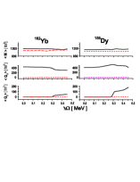
Figure 1: (Color online) The rotational behaviour of the calculated monopole and quadrupole moments. The ”double-stretched” and standard values are connected by dashed and solid line, respectively.

The results of our calculations conform to the results of the Nilsson+Strutinsky shell correction method (compare our Fig.2 with Fig.3c in Ref.Kon, ), although we obtain slightly different values for the equilibrium deformations. In the analysis of Ref.Kon, the pairing correlations are omitted. In addition, in the Nilsson+Strutinsky shell correction method the rigid body moment of inertia simulates the inertial nuclear properties, which is different from the microscopic one, even at high spin region (see below). Moreover, the use of the Nilsson+Strutinsky results destroys the self-consistency between the mean-field calculations and the RPA analysis. Therefore, to keep a self-consistency between the mean field and the RPA as much as possible, we use the recipe described above.

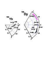
Figure 2: Equilibrium deformations in $\beta$-$\gamma$ plane as a function of the angular momentum $I=\langle{\hat{J}}_{x}\rangle-1/2$ (in units of $\hbar$). The equilibrium deformations for ¹⁵⁶Dy provide the lower mean field energies in the region $-\pi/3<\gamma<0$ (filled circles) in comparison with those (open squares) obtained in Ref.JK05, . The both branches of the equilibrium deformations are obtained enforcing the condition Eq.(7). The maximal difference between the minimal HB energies at the positive and negative equilibrium $\gamma$-values does not exceed $\sim 1$MeV for ¹⁵⁶Dy.

The triaxiality of the mean field sets in at the critical rotational frequency $\Omega_{c}$ which triggers the backbending in the considered nuclei due to different mechanisms. As shown in Fig.2, we obtain the critical rotational frequencies, at which the first band crossing occurs, $\hbar\Omega_{c}\approx 0.25$MeV $(10\hbar\rightarrow 12\hbar)$ for ¹⁶²Yb and $\hbar\Omega_{c}\approx 0.3$MeV $(14\hbar\rightarrow 16\hbar)$ for ¹⁵⁶Dy. The contribution of the additional term, Eq.(II.1), was crucial to achieve a good correspondence between the calculated and experimental values of the crossing frequency in each nucleus (see discussion in Ref.JK05, ).

In ¹⁵⁶Dy we obtain that the $\gamma$-vibrational excitations ($K=2$) of the positive signature tends to zero in the rotating frame at the transition point, in close agreement with experimental data. At the transition point there are two indistinguishable HB minima with different shapes: axially symmetric and strongly nonaxial. It is interesting to note that this behaviour is symmetric with respect to the sign of the $\gamma$-deformation, although the difference between the HB energy minima for $\gamma=\pm 20^{0}$ is about $\sim 0.8$MeV. The increase of the rotational frequency changes the axial shape to the nonaxial one with a negative $\gamma$-deformation ($\gamma\sim-20^{o}$). The transition possesses all features of the shape-phase transition of the first order. One may expect the appearance of the wobbling excitations near the transition point, since after a shape transition there is a strong nonaxiality in ¹⁵⁶Dy. In contrast with ¹⁵⁶Dy, in ¹⁶²Yb the axially symmetric configuration is replaced by the two-quasiparticle one with a small negative $\gamma$-deformation. There, the backbending takes place due to the rotational alignment of a neutron $i_{13/2}$ quasiparticle pair. The nonaxiality evolves quite smoothly, exhibiting the main features of the shape-phase transition of the second order. The question arises how is reliable our description or how self-consistently are done our mean field calculations ?

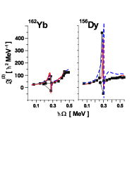
Figure 3: (Color online) The rotational dependence of the dynamic $\Im_{HB}^{(2)}=-d^{2}E_{HB}/d\Omega^{2}=d\langle{\hat{J}}_{x}\rangle/d\Omega$ (a solid line) and the Thouless-Valatin $\Im_{TV}$ moments of inertia (a dash line). The experimental values $\Im^{(2)}=4/\Delta E_{\gamma}$ are denoted by filled square connected by a thin line to guide eye. Here, $\Delta E_{\gamma}$ is the difference between two consecutive $\gamma$-transitions, and $E_{\gamma}$ is the $\gamma$-transition energy between two neighboring states that differ on two units of the angular momentum

One of the conclusive tests of the self-consistency microscopic calculations is the comparison of the dynamic moment of inertia $\Im_{HB}^{(2)}$, calculated in the mean field approximation, and the Thouless-Valatin moment of inertia $\Im_{TV}$, calculated in the RPA. They must coincide (see the results for exactly solvable model in Ref.n2, ), if one found a self-consistent mean field minimum and spurious solutions are separated from the physical ones. Our results (see Fig.3) demonstrate a good self-consistency between the mean field and the CRPA calculations, indeed (see also the discussion in Ref.JK05, ). We emphasize that the inclusion of the correction term, Eq.(II.1), is crucial to achieve a good description of the inertial nuclear properties.

II.2 Negative signature excitations

To describe quantum oscillations around mean field solutions the boson-like operators $b^{+}_{k\bar{l}}=\alpha^{+}_{k}\alpha^{+}_{\bar{l}},b^{+}_{kl}=\alpha^{+}_{k}\alpha^{+}_{l},b^{+}_{\bar{k}\bar{l}}=\alpha^{+}_{\bar{k}}\alpha^{+}_{\bar{l}}$ are used. The first equality introduces the positive signature boson, while the other two determine the negative signature ones. These two-quasiparticle operators are treated in the quasi-boson approximation (QBA) as an elementary bosons, i.e., all commutators between them are approximated by their expectation values with the uncorrelated HB vacuum RS . The corresponding commutation relations can be found in Ref.KN, . In this approximation the positive and negative signature boson spaces are not mixed, since the corresponding operators commute and $H_{\Omega}=H_{\Omega}(r=+1)+H_{\Omega}(r=-1)$. The analysis of the positive signature term $H_{\Omega}(r=+1)$ is done in Ref.JK05, .

In the UR frame, the negative signature RPA Hamiltonian has the form

$$\hat{H}_{\Omega}[r=-1]=\frac{1}{2}\sum_{\mu}E_{\mu}b^{+}_{\mu}b_{\mu}-\frac{\chi}{2}\sum_{\mu_{3}=1,2}\tilde{Q}^{(-)2}_{\mu_{3}}\,,$$ (9)

where $E_{\mu}=\varepsilon_{i}+\varepsilon_{j}$ ($E_{\bar{i}\bar{j}}=\varepsilon_{\bar{i}}+\varepsilon_{\bar{j}}$) are two-quasiparticle energies. Hereafter, we use the following definitions: the index $\mu$ runs over $ij$, $\bar{i}\bar{j}$ and the index $\mu_{3}$ is a projection on the quantization axis z. The double stretched quadrupole operators $\tilde{Q}_{1}^{(-)}=\xi{\hat{Q}}_{1}^{(-)}$ ($\xi=\omega_{x}\omega_{z}/\omega_{0}^{2}$), $\tilde{Q}_{2}^{(-)}=\eta{\hat{Q}}_{2}^{(-)}$ ($\eta=\omega_{x}\omega_{y}/\omega_{0}^{2}$) are defined by means of the quadrupole operators ${\hat{Q}}_{m}^{(r)}$ (m=0,1,2)

$$\hat{Q}_{m}^{(r)}=\frac{i^{2+m+(r+3)/2}}{\sqrt{2(1+\delta_{m0})}}\biggl{(}\hat{Q}_{2m}+(-1)^{(r+3)/2}\hat{Q}_{2-m}\biggr{)},$$ (10)

where $\hat{Q}_{\lambda m}={\hat{r}}^{\lambda}Y_{\lambda m}$. We recall that the residual doubly-stretched interaction does not distort the mean field deformations found self-consistently for the Hamiltonian (1). The violation of the self-consistency leads, however, to unreliable description of the vibrational states.

The RPA Hamiltonian (9) contains only the isoscalar part of the quadrupole interaction, since we would like to establish a connection between the microscopic approach and the phenomenological ARM to see evidently similarities and differences. Moreover, in the considered nuclei the main contribution of the isovector quadrupole-quadrupole interaction is located in energy region around $\sim 3$MeV and is responsible for M1 excitations JK2 . One should keep in mind, however, that the isovector part of the quadrupole interaction may be important for the analysis of wobbling excitations in odd-odd nuclei, when there is a different orientation of the neutron and proton s.p. high-j orbitals and strong $M1$-transitions are observed along yrast and/or yrare states. The spin-spin interaction, $V_{\sigma\sigma}=-\frac{1}{2}\sum_{T=0,1}\kappa_{\sigma}(T)\sum_{r=\pm}\sum_{\mu=0,1}(s_{\mu}[^{T}_{r}])^{2}$ (see the discussion in Refs.JK2, ; JK05, ) is not essential for low-lying quadrupole vibrations and is omitted in our analysis. The pairing interaction does not contribute to the boson Hamiltonian, $\hat{H}_{\Omega}[r=-1]$, since it is of the positive signature. Notice, however, that the matrix elements of the operators depend on the pairing interaction which affects the RPA solutions.

The linear boson part of the double stretched operators has the following form

$$\tilde{Q}_{1}^{(-)} = -\frac{1}{2}\sum_{\mu}\tilde{f_{1\mu}}(b^{+}_{\mu}+b_{\mu}),\quad\tilde{f_{1\mu}}=\xi q_{1\mu}$$ (11)

$$\tilde{Q}_{2}^{(-)} = -\frac{i}{2}\sum_{\mu}\tilde{f_{2\mu}}(b^{+}_{\mu}-b_{\mu}),\quad\tilde{f_{2\mu}}=\eta q_{2\mu}$$ (12)

Here, $q_{1\mu}$, $q_{2\mu}$ are real matrix elements of the operators ${\hat{Q}}_{1}^{(-)}$, ${\hat{Q}}_{2}^{(-)}$, respectively (the properties of matrix elements of the operators involved in the Hamiltonian (9) can be found in Ref.JK, ).

We solve the RPA equations of motion

$$[\hat{H}_{\Omega},\hat{P}_{\nu}]\, = \,i\,\omega_{\nu}\,\hat{X}_{\nu},\qquad[\hat{H}_{\Omega},\hat{X}_{\nu}]\,=\,-i\,\omega_{\nu}\,\hat{P}_{\nu},$$ (13)

$$[\hat{X}_{\nu},\hat{P}_{\nu^{\prime}}]\,=\,i\delta_{\nu\,\nu^{\prime}},$$

where

$$\hat{X}_{\nu}=\sum_{\mu}X^{\nu}_{\mu}(b^{+}_{\mu}+b_{\mu}),\quad\hat{P}_{\nu}=i\sum_{\mu}P^{\nu}_{\mu}(b^{+}_{\mu}-b_{\mu})$$ (14)

are, respectively, the collective coordinates and their conjugate momenta (hereafter, we use in all equations $\hbar=1$). The RPA eigenfunction

$$|\nu\rangle = \hat{O}_{\nu}^{\dagger}|RPA\rangle=\frac{1}{\sqrt{2}}\,\Bigl{(}\,\hat{X}_{\nu}\,-\,i\hat{P}_{\nu}\,\Bigr{)}|RPA\rangle$$ (15)

$$= \sum_{\mu}(\psi^{(\nu)}_{\mu}b^{+}_{\mu}-\phi^{(\nu)}_{\mu}b_{\mu})|RPA\rangle$$

defines the amplitudes $\psi^{(\nu)}_{\mu}$ and $\phi^{(\nu)}_{\mu}$ by means of the generalized coordinate and momentum amplitudes. The ket vector $\mid RPA\rangle$ denotes the RPA vacuum (yrast state) at the rotational frequency $\Omega$.

The solution of the above equations (13) determines the generalized coordinate and momentum amplitudes

$$X_{\mu}^{\nu}=\chi{\tilde{R}}^{\nu}_{1}\frac{\omega_{\nu}{\tilde{f}}_{1\mu}}{E_{\mu}^{2}-\omega_{\nu}^{2}}+\chi{\tilde{R}}^{\nu}_{2}\frac{E_{\mu}{\tilde{f}}_{2\mu}}{E_{\mu}^{2}-\omega_{\nu}^{2}}$$

$$P_{\mu}^{\nu}=\chi{\tilde{R}}^{\nu}_{1}\frac{E_{\mu}{\tilde{f}}_{1\mu}}{E_{\mu}^{2}-\omega_{\nu}^{2}}+\chi{\tilde{R}}^{\nu}_{2}\frac{\omega_{\nu}{\tilde{f}}_{2\mu}}{E_{\mu}^{2}-\omega_{\nu}^{2}}$$ (16)

with unknown coefficients

$${\tilde{R}}^{\nu}_{1}=\sum_{\mu}{\tilde{f}}_{1\mu}P^{\nu}_{\mu}\equiv-\frac{1}{\sqrt{2}}\left[\hat{O}_{\nu},\tilde{Q}_{1}^{(-)}\right]$$

$${\tilde{R}}^{(\nu)}_{2}=\sum_{\mu}{\tilde{f}}_{2\mu}X^{\nu}_{\mu}\equiv\frac{i}{\sqrt{2}}\left[\hat{O}_{\nu},\tilde{Q}_{2}^{(-)}\right]$$ (17)

and eigenvalues $\omega_{\nu}$. To find the eigenvalues $\omega_{\nu}$ one transforms the system Eq.(16) to the form

$${\tilde{R}}^{\nu}_{1}\left[D_{11}(\omega_{\nu})-\frac{1}{\chi}\right]+{\tilde{R}}^{\nu}_{2}D_{12}(\omega_{\nu}) = 0$$

$${\tilde{R}}^{\nu}_{1}D_{12}(\omega_{\nu})+{\tilde{R}}^{\nu}_{2}\left[D_{22}(\omega_{\nu})-\frac{1}{\chi}\right] = 0$$ (18)

The condition

$$F(\omega_{\nu})=\det~{}({\bf D}-\frac{\bf 1}{\chi})=0$$ (19)

determines all negative signature RPA solutions. The matrix elements $D_{km}(\omega_{\nu})=\sum_{\mu}{\tilde{f}}_{k,\mu}{\tilde{f}}_{m,\mu}C_{\mu}^{km}/(E_{\mu}^{2}-\omega_{\nu}^{2})$ involve the coefficients $C_{\mu}^{km}=\omega_{\nu}$ for $k\neq m$ and $E_{\mu}$ otherwise. Although the determinant has a dimension $n=2$, one obtains a huge family of RPA solutions with different degree of the collectivity. Among collective solutions there are solutions that correspond to the shape fluctuations of the system. Notice that the direction of the angular momentum is fixed in the UR frame.

III The wobbling mode

III.1 Janssen-Mikhailov equation

We recall that the doubly-stretched residual interaction restores in the RPA the rotational symmetry broken at the mean field approximation. Therefore, for the cranking Hamiltonian the conservation laws imply in the RPA order

$$[\,H_{\Omega}\,,\,\hat{J}_{y}\mp i\hat{J}_{z}\,]\,=\pm\Omega(\hat{J}_{y}\mp i\hat{J}_{z})$$ (20)

This condition is equivalent to the condition of the existence of the negative signature solution $\omega_{\nu}=\Omega$ created by the operator (see Ref.mar3, )

$$\hat{\Gamma}^{\dagger}=\frac{\hat{J}_{z}+i\hat{J}_{y}}{\sqrt{2\langle\hat{J}_{x}\rangle}},\quad\hat{\Gamma}=(\hat{\Gamma}^{\dagger})^{\dagger},\quad[\hat{\Gamma},\hat{\Gamma}^{\dagger}]=1$$ (21)

This operator describes a collective rotational mode in the subspace of $\hat{H}_{\Omega}(-)$

$$[\hat{H}_{\Omega}(-),\hat{\Gamma}^{\dagger}]=\Omega\hat{\Gamma}^{\dagger},$$ (22)

arising from the symmetries broken by the external rotational field (the cranking term).

This is true for a pure harmonic oscillator model only n2 . However, our Hamiltonian (1) contains the additional term $h_{add}$, Eq.(II.1). Since the additional term $h_{add}$ has a term proportional to $\hat{l}_{x}$-operator, the conservation laws (20) are broken for the Hamiltonian (1). Nevertheless, these laws can be fulfilled in the RPA order by changing the strength constant in Eq.(19) in order to obtain the solution $\omega_{\nu}=\Omega$ JK05 . To check this fact, we calculated the RPA secular equation (19) for the mode $\omega_{\nu}=\Omega$, with and without the additional term $h_{add}$, for the same strength constant (see also Fig.10 in Ref.JK05, )). The results evidently demonstrate that the conservation laws (20), (22) are fulfilled with a good accuracy (see Fig.4). In fact, due to a smallness of the term proportional to the operator $\hat{l}_{x}$ in the additional term, the violation is almost negligible.

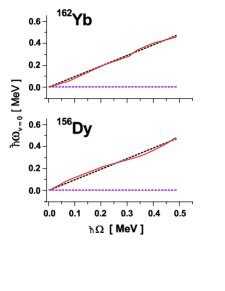
Figure 4: (Color online) The evolution of the negative signature RPA solution $\omega_{\nu}=\Omega$ with (dashed line) and without (solid line) the additional term Eq.(II.1) as function of the rotational frequency, calculated at the equilibrium deformations (see Fig.2). The straight dashed line, parallel to the $\hbar\Omega$-axis, denotes the yrast line.

Based on this fact, we exploit the conservation laws (20) for the Hamiltonian (9), that yield the following equations

$$\Omega J^{z}_{\mu}+E_{\mu}J^{y}_{\mu}=\chi\xi A{\tilde{f}}_{1\mu}$$ (23)

$$\Omega J^{y}_{\mu}+E_{\mu}J^{z}_{\mu}=\chi\eta B{\tilde{f}}_{2\mu}$$ (24)

We will see below that these equations are fulfilled with a good numerical accuracy, since the redundant mode is separated from the other RPA solutions by our procedure for the strength constant. The parameters $A$ and $B$

$$\xi A=\langle\,[{\tilde{Q}}_{1}^{(-)}\,,\,iJ_{y}\,]\rangle=\sum_{\mu}{\tilde{f}}_{1\mu}J_{\mu}^{y}=\xi\langle Q_{2}+\sqrt{3}Q_{0}\rangle$$ (25)

$$\eta B=\langle\,[{\tilde{Q}}_{2}^{(-)}\,,\,-iJ_{z}\,]\rangle=\sum_{\mu}{\tilde{f}}_{2\mu}J_{\mu}^{z}=2\eta\langle Q_{2}\rangle$$ (26)

are obtained with the aid of the commutator $[\hat{J}_{x}\pm i\hat{J}_{y},\hat{Q}_{\lambda m}]=\sqrt{\lambda(\lambda+1)-m(m\pm 1)}\hat{Q}_{\lambda m\pm 1}$ (see Ref.var, ). The above relations between the matrix elements, Eqs.(23),(24), are a key point for the analysis of the wobbling excitations at nonzero $\gamma$-deformation, i.e., $\langle Q_{2}\rangle\neq 0$. Moreover, in virtue of the definitions for the phonon operator (Eqs.(15),(16)) and the operator $\hat{\Gamma}$ (Eq.(21)), employing Eqs.(23),(24), and Eq.(33) below, one can show that

$$[\hat{\Gamma},\hat{O}_{\nu}]=[\hat{\Gamma},\hat{O}_{\nu}^{\dagger}]=0$$ (27)

Following the procedure described in Ref.JM79, , with the aid of Eqs.(23),(24), one arrives to the equation

$$(\omega_{\nu}^{2}-\Omega^{2}){\Delta}(\omega_{\nu})=0$$ (28)

The determinant ${\Delta}(\omega_{\nu})$ corresponds to the system of equations

$$\omega_{\nu}S_{y}r_{1}^{\nu}-\Omega{\Im}_{xy}r_{2}^{\nu}=0$$

$$\Omega{\Im}_{xz}r_{1}^{\nu}-\omega_{\nu}S_{z}r_{2}^{\nu}=0$$ (29)

for unknowns

$$r_{1}^{\nu}=\frac{\tilde{R}_{1}^{\nu}}{(\xi A)},\quad r_{2}^{\nu}=\frac{\tilde{R}_{2}^{\nu}}{(\eta B)},$$ (30)

that does not contain anymore the solution $\omega_{\nu}=\Omega$. We introduced above the following notations

$${\Im}_{xy} = \Im_{x}-\Im_{y}-\omega_{\nu}^{2}S/{\Omega}$$

$${\Im}_{xz} = \Im_{x}-\Im_{z}-\omega_{\nu}^{2}S/{\Omega}$$ (31)

$$S_{y,z} = {\Im}_{y,z}+\Omega S\qquad,$$

where

$$S=\sum_{\mu}\frac{J^{y}_{\mu}J^{z}_{\mu}}{E^{2}_{\mu}-\omega_{\nu}^{2}},\quad\Im_{y,z}=\sum_{\mu}\frac{E_{\mu}{(J^{y,z}_{\mu}})^{2}}{E^{2}_{\mu}-\omega_{\nu}^{2}}$$ (32)

and $\Im_{x}=\langle\hat{J}_{x}\rangle/\Omega$ is the definition of the kinematic moment of inertia. From the system (29), one obtains the relations between unknowns $r_{1}^{\nu}$ and $r_{2}^{\nu}$

$$\frac{r_{1}^{\nu}}{r_{2}^{\nu}}=\frac{\Omega{\Im}_{xy}}{\omega_{\nu}S_{y}}=\frac{\omega_{\nu}S_{z}}{\Omega{\Im}_{xz}},$$ (33)

which are helpful for our analysis below.

The condition ${\Delta}(\omega_{\nu})=0$ leads to the Janssen-Mikhailov equation JM79

$${\Delta}(\omega_{\nu})=\omega_{\nu}^{2}-\Omega^{2}\frac{[\Im_{x}-\Im_{y}-\omega_{\nu}^{2}S/{\Omega}][\Im_{x}-\Im_{z}-\omega_{\nu}^{2}S/{\Omega}]}{[\Im_{y}+\Omega S][\Im_{z}+\Omega S]}=0,$$ (34)

that determines all vibrational modes of the negative signature excluding the solution $\omega_{\nu}=\Omega$. We stress that the solution of this equation alone is meaningless. While Eq.(34) does not depend on the strength constant, the violation of the conditions (23),(24), by arbitrary variation of the $\gamma$-deformation or pairing gap destroys the link between the systems, Eq.(II.2) and Eq.(29). As a result, the redundant mode can not be removed from Eq.(19) and one is not able to obtain Eq.(34). Providing the wobbling solution, this equation has, however, a different form than the Bohr-Mottelson classical equation. Below we present a simple derivation of the microscopic analog of the latter one.

III.2 Marshalek moments of inertia

The relations Eq.(33) are equivalent to the following ones

$$\frac{r_{1}^{\nu}S_{y}}{r_{2}^{\nu}S_{z}}=\frac{\Omega{\Im}_{xy}}{\omega_{\nu}S_{z}}=\frac{\omega_{\nu}S_{y}}{\Omega{\Im}_{xz}}$$ (35)

These relations can be associated with the system of equations

$$\omega_{\nu}S_{z}a-\Omega{\Im}_{xy}b=0$$

$$\Omega{\Im}_{xz}a-\omega_{\nu}S_{y}b=0$$ (36)

for unknowns $a=r_{1}^{\nu}S_{y}$ and $b=r_{2}^{\nu}S_{z}$. With the aid of definitions, Eqs.(31), we rearrange this system to the following form

$$\omega_{\nu}(\Im_{z}+\omega_{\nu}S\frac{b}{a})a-\Omega(\Im_{x}-\Im_{y}-\omega_{\nu}S\frac{a}{b})b=0$$

$$\Omega(\Im_{x}-\Im_{z}-\omega_{\nu}S\frac{b}{a})a-\omega_{\nu}(\Im_{y}+\omega_{\nu}S\frac{a}{b})b=0$$ (37)

In virtue of the relations, Eqs.(35), between the unknowns $a$ and $b$, we define the effective moments of inertia in the UR frame

$$\Im_{2}^{\it eff}=\Im_{y}+\omega_{\nu}S\frac{a}{b}=\Im_{y}+\Omega S\frac{\Im_{xy}}{S_{z}}$$

$$\Im_{3}^{\it eff}=\Im_{z}+\omega_{\nu}S\frac{b}{a}=\Im_{z}+\Omega S\frac{\Im_{xz}}{S_{y}}$$ (38)

that depend on the RPA frequency. The definitions (38) are the same as those obtained by Marshalek in the time-dependent Hartree-Bogoliubov approach but in the PA frame mar2 . The determinant for nonzero solutions of the system Eq.(37) yields the nonlinear equation similar to the classical expression for the wobbling mode BM75

$$\omega_{\nu=w}=\Omega\sqrt{\frac{[\Im_{x}-\Im^{\it eff}_{2}][\Im_{x}-\Im^{\it eff}_{3}]}{\Im^{\it eff}_{2}\Im^{\it eff}_{3}}}\,,$$ (39)

with the microscopically defined moments of inertia. Eq.(39) was obtained first by Marshalek in the PA frame from the equations for the amplitudes of the angular frequency time oscillations. In the UR (time-independent) frame we obtain this equation with much less efforts as well.

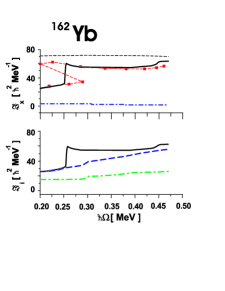
Figure 5: (Color online) ¹⁶²Yb. Top panel: the kinematic moment of inertia ${\Im}_{x}=\langle{\hat{J}}_{x}\rangle/\Omega$ (solid line), a rigid body (dashed line) and a hydrodinamical moments of inertia (dash-dotted line) are compared with the experimental values (filled squares). Experimental values ${\Im}_{x}=I/\Omega$ are connected by dashed line to guide eyes ($\hbar\Omega=E_{\gamma}/2$). Bottom panel displays the rotational dependence of the kinematic moment of inertia (solid line), Marshalek moments of inertia $\Im^{\it eff}_{2}$ (dashed line) and $\Im^{\it eff}_{3}$ (dash-dotted line) for the first RPA solution $\nu=1$ obtained from Eq.(19).

It is evident that for the rotation around the axis x the wobbling excitations with different collectivity could be found from Eq.(39), if the condition

$$\Im_{x}>\Im^{\it eff}_{2},\Im^{\it eff}_{3}\quad(or\quad\Im_{x}<\Im^{\it eff}_{2},\Im^{\it eff}_{3})$$ (40)

is fulfilled. One may expect that for the RPA solutions, different from the wobbling mode, this condition should not hold. Notice that Eq.(19) contains the solutions to Eq.(39) but not vise versa, since the above constraint, Eq.(40), valid for the later case, is not required for the former one.

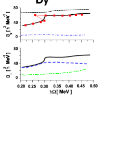
Figure 6: (Color online) ¹⁵⁶Dy. Similar to Fig.5.

We obtain quite a remarkable correspondence between the experimental and calculated values for the kinematic moment of inertia for the both nuclei (see top panels in Figs.5,6). We trace also the evolution of the irrotational fluid moment of inertia (see Ref.RS, )

$$\Im^{(irr)}_{i}=\frac{3}{2\pi}mAR^{2}\beta^{2}\sin^{2}\left(\gamma-\frac{2\pi}{3}i\right)$$ (41)

and a rigid body moment of inertia $(i=1,2,3)$

$$\Im^{(rig)}_{i}=\frac{2}{5}mAR^{2}\left(1-\sqrt{\frac{5}{4\pi}}\beta\cos(\gamma-\frac{2\pi}{3}i)\right)$$ (42)

as a function of the equilibrium deformations (see Fig.2). The irrotational fluid moment of inertia $\Im^{(irr)}_{1}$ does not reproduce neither the rotational dependence nor the absolute values of the experimental one as a function of the rotational frequency. The rigid body values provide the asymptotic limit of fast rotation without pairing. Evidently, the difference between the rigid body and the calculated kinematic moments of inertia in the both nuclei decreases with the increase of the rotational frequency, although it remains visible at high spins. At very fast rotation $\hbar\Omega>0.45$MeV the pairing correlations are reduced due to multiple alignments, and, therefore, the difference is moderated.

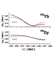
Figure 7: (Color online) The rotational dependence of the RPA solutions, obtained with the aid of Eq.(19) (solid line) and Eq.(39) (dashed line). The RPA solutions, obtained with the aid of Eq.(19), fulfil the condition Eq.(40).

The calculated values of the Marshalek moments of inertia, Eq.(38), signal (see the bottom panels, Figs.5,6) that one should expect the appearance of the wobbling mode after a shape-phase transition in ¹⁶²Yb and ¹⁵⁶Dy for the first RPA solution found with the aid Eq.(19). As was stressed above, the separation of the redundant mode is an essential point for the RPA wobbling theory, that secures a reliable analysis of the RPA modes. Additionally, to be assure in the self-consistency of our RPA calculations, we compare the solutions, that may be associated with wobbling excitations, from different RPA equations (19) and (39). We recall that Eq.(19) depends on the strength constant $\chi$ and contains different RPA solutions including the redundant mode, while this dependence is removed from Eq.(39). Evidently, if the redundant mode would not be removed from Eq.(19) by our choise of the strength constants, the conditions Eqs.(23),(24) should be broken. As a result, the consistency between Eq.(19) and Eq.(39) would be broken as well and these equations would provide different solutions. A nice agreement between the roots of Eq.(19) and Eq.(39) (see Fig.7) confirms the vitality and the validity of our approach.

Does the constraint (40) guarantee the existence of a collective wobbling mode solution ? Below we formulate criteria how to identify the collective wobbling excitations.

III.3 Criteria for wobbling excitations

By means of Eqs.(37),(38), we can define the unknown variables $r_{1}^{\nu=w}=a/S_{y}$, $r_{2}^{\nu=w}=b/S_{z}$ (which determine the wobbling mode) such that

$$\frac{r_{1}^{w}}{r_{2}^{w}} = \frac{S_{z}}{S_{y}}\frac{a}{b}=\frac{S_{z}}{S_{y}}\frac{\Omega(\Im_{x}-\Im^{\it eff}_{2})}{\omega_{w}\Im^{\it eff}_{3}}=$$ (43)

$$= \frac{S_{z}}{S_{y}}\frac{\omega_{w}\Im^{\it eff}_{2}}{\Omega(\Im_{x}-\Im^{\it eff}_{3})}=\sqrt{\frac{W_{2}}{W_{3}}}\frac{S_{z}}{S_{y}}\frac{\Im^{\it eff}_{2}}{\Im^{\it eff}_{3}}$$

Here, we used the fact that the dispersion equation for the wobbling mode, Eq.(39), can be expressed as $\omega_{w}=\langle{\hat{J}}_{x}\rangle\sqrt{W_{2}W_{3}}$, where

$$W_{2}=(1/\Im_{2}^{\it eff}-1/\Im_{x}),\quad W_{3}=(1/\Im_{3}^{\it eff}-1/\Im_{x})$$ (44)

With the aid of Eqs.(38) and the definition, Eqs.(31), it is easy to show that the ratio $S_{z}\Im^{\it eff}_{2}/S_{y}\Im^{\it eff}_{3}\equiv 1$. It results in the following relation

$$\frac{r_{1}^{w}}{r_{2}^{w}}=\sqrt{\frac{W_{2}}{W_{3}}}$$ (45)

Our next task is to find a formal expressions for the unknowns $r_{1,2}^{w}$ in terms of the functions $W_{2,3}$ that depend on the microscopic moments of inertia.

By means of the inverse transformation

$$b_{\mu}^{\dagger}=\sqrt{2}\sum_{\nu}X_{\mu}^{\nu}(\hat{O}_{\nu}^{\dagger}-\hat{O}_{\nu})+P_{\mu}^{\nu}(\hat{O}_{\nu}^{\dagger}+\hat{O}_{\nu})$$ (46)

we can express the operators $\tilde{Q}_{1,2}^{(-)}$ (see Eqs.(11),(12), (17)) via phonon operators

$$\tilde{Q}_{1}^{(-)}=-\sqrt{2}\sum_{\nu}{\tilde{R}}_{1}^{\nu}(\hat{O}_{\nu}^{\dagger}+\hat{O}_{\nu})$$ (47)

$$\tilde{Q}_{2}^{(-)}=-i\sqrt{2}\sum_{\nu}{\tilde{R}}_{2}^{\nu}(\hat{O}_{\nu}^{\dagger}-\hat{O}_{\nu})$$ (48)

Let us use the fact that the components of the quadrupole tensor commute, i.e., the condition

$$\left[\tilde{Q}_{1}^{(-)},\tilde{Q}_{2}^{(-)}\right]=4i\sum_{\nu={\it all}}{\tilde{R}}_{1}^{\nu}{\tilde{R}}_{2}^{\nu}$$

$$=2\sum_{\nu={\it all}}\left[{\hat{D}}_{\nu},\tilde{Q}_{1}^{(-)}\right]\left[{\hat{D}}_{\nu},\tilde{Q}_{2}^{(-)}\right]=0$$ (49)

Here, we use the notation ${\hat{D}}_{\nu=\Omega}\equiv{\hat{\Gamma}}$ and ${\hat{D}}_{\nu\neq\Omega}\equiv{\hat{O}}_{\nu}$ for other vibrational modes. Taking into account the definitions Eqs.(17),(30) (see also Eqs.(21),(25),(26)), we obtain the exact definitions for the unknowns $r_{1,2}^{\Omega}$ associated with the redundant mode:

$$r_{1}^{\Omega}=\frac{{\tilde{R}}_{1}^{\nu=\Omega}}{\xi A}=-\frac{1}{\xi A\sqrt{2}}\left[{\hat{\Gamma}},\tilde{Q}_{1}^{(-)}\right]=-\frac{1}{2\sqrt{\langle\hat{J}_{x}\rangle}},$$

$$r_{2}^{\Omega}=\frac{{\tilde{R}}_{2}^{\nu=\Omega}}{\eta B}=\frac{i}{\eta B\sqrt{2}}\left[{\hat{\Gamma}},\tilde{Q}_{2}^{(-)}\right]=\frac{1}{2\sqrt{\langle\hat{J}_{x}\rangle}}$$ (50)

This result yields the following expression for the sum, Eq.(49),

$$\sum_{\nu\neq w,\Omega}r_{1}^{\nu}r_{2}^{\nu}+r_{1}^{w}r_{2}^{w}=-r_{1}^{\Omega}r_{2}^{\Omega}=\frac{1}{4\langle\hat{J}_{x}\rangle}$$ (51)

Suppose, that in the l.h.s of Eq.(51) the sum, defined by all physical solutions excluding the wobbling one, is zero due to a mutual cancellation of different terms. Below, we will see that it is, indeed, the case. As a result, we obtain the equation for the unknowns $r_{1,2}^{w}$. Resolving this equation by dint of Eq.(45), we obtain

$$r_{1}^{w}=\frac{1}{2\sqrt{\langle\hat{J}_{x}\rangle}}\left(\frac{W_{2}}{W_{3}}\right)^{1/4},\quad r_{2}^{w}=\frac{1}{2\sqrt{\langle\hat{J}_{x}\rangle}}\left(\frac{W_{3}}{W_{2}}\right)^{1/4}$$ (52)

These expressions are similar to those of the wobbling mode in the Bohr-Mottelson model (see Appendix, Eqs.(A.14)), although the quantities $W_{2,3}$ are determined by the Marshalek moments of inertia and $\langle\hat{J}_{x}\rangle\simeq I+1/2$ (the factor $1/2$ is arising due to the RPA contribution of the redundant mode, see discussion in Ref.al, ). Note that similar expressions were obtained in Ref.shi1, in the PA frame (with the quantization condition $\langle\hat{J}_{x}\rangle=I$ and some additional phases).

To identify the wobbling mode among the solutions of Eq.(19) it is convenient to transform Eq.(49) to the form

$$\sum_{\nu=all}c_{\nu}=0,\quad c_{\nu}=4\langle\hat{J}_{x}\rangle\frac{{\tilde{R}}_{1}^{\nu}}{\xi A}\frac{{\tilde{R}}_{2}^{\nu}}{\eta B}$$ (53)

From Eqs.(50), (52) it follows that

$$c_{\nu=\Omega}\equiv-1,\quad c_{\nu=w}\equiv 1$$ (54)

Thus, solving only the system of the RPA equations for the quadrupole operators, Eq.(19), the condition Eq.(54) enables us to identify the redundant and the wobbling modes.

III.4 Analysis of experimental data

The experimental level sequences for all observed up-to-date rotational bands in ${}^{162}Yb$ and ¹⁵⁶Dy are taken from Ref.nndc, , which is regularly updated. The rotational bands are numerated as rotational bands B1, B2… in accordance with nndc . All rotational states are classified by the quantum number $\alpha$ which is equivalent to our signature $r$. The positive signature states ($r=+1$) correspond to $\alpha=0$, since the quantum number $\alpha$ leads to selection rules for the total angular momentum $I=\alpha+2n$, $n=0,\pm 1,\pm 2\ldots$ (cf Ref.fra, ). In particular, in even-even nuclei the yrast band characterized by the positive signature quantum number $r=+1\,(\alpha=0)$ consists of even spins only. The negative signature states ($r=-1$) correspond to $\alpha=1$ and are associated with odd spin states in even-even nuclei. All considered bands are of the positive parity $\pi=+$.

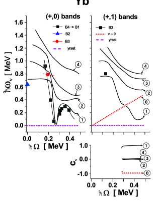
Figure 8: (Color online)¹⁶²Yb. Top left panel: the rotational dependence of the positive signature RPA solutions with even spins $(\pi=+,\alpha=0)$. Number in a circle denotes the RPA solution number : $1$ is the first $\nu=1$ RPA solution etc. Different symbols display the experimental data associated with B1,B2…bands (the band labels are taken in accordance with the definitions given in Ref.nndc, ). Top right panel: the rotational dependence of the negative signature RPA solutions with odd spins $(\pi=+,\alpha=1)$. The redundant mode $\omega_{\nu}=\Omega$ is denoted as ”0” and is displayed by the dotted line. Bottom panel: the rotational dependence of the coefficients $c_{\nu}\sim\tilde{R}_{1}^{\nu}\tilde{R}_{2}^{\nu}$ (see Eq.(53)) that are determined by the solutions of Eq.(19).

Before to make a comparison of our results with the data, let us analyse RPA solutions in order to identify a wobbling mode. Top right panels of Figs.8, 9 display four lowest RPA solutions of Eq.(19) and the redundant mode of Eq.(19) as a function of the rotational frequency. We recall that these solutions are found at different equilibrium deformations (see Fig.2). Indeed, in the both nuclei the criteria Eq.(54) uniquely determines the redundant and the wobbling modes. In Figs.8, 9 the redundant mode is manifested as a straight line (see the top right panels), while the corresponding coefficient $c_{\Omega}$ is always -1 (the bottom panels). The rotational mode is separated clearly from the vibrational modes. Notice that the solutions, that are different from rotational and wobbling modes, contribute to the sum Eq.(51) with a zero weight, as it was proposed above.

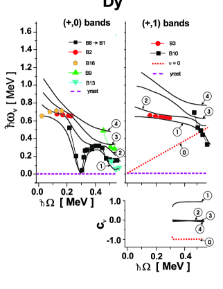
Figure 9: (Color online)¹⁵⁶Dy. The same as for Fig.8.

To compare our results with available experimental data on low lying excited states near the yrast line nndc we construct the Routhian function for each rotational band $\nu$ ($\nu=yrast,\beta,\gamma,...$)

$$R_{\nu}(\Omega)=E_{\nu}(\Omega)-\hbar\Omega I(\Omega),\quad\quad\Omega(I)=\frac{E_{\nu}(I+1)-E_{\nu}(I-1)}{2}$$ (55)

and define the experimental excitation energy in the rotating frame $\hbar\omega_{\nu}^{\it exp}=R_{\nu}(\Omega)-R_{yr}(\Omega)$ n87 . In ¹⁶²Yb it is known only one negative signature $\gamma$-vibrational state. The first RPA solution ($\nu=1$) is a negative signature gamma-vibrational mode (with odd spins) till $\hbar\Omega\approx 0.28$MeV. With the increase of the rotational frequency it is transformed to the wobbling mode at $\hbar\Omega\approx 0.32$MeV (according to the criterion Eq.(54)). The other solutions ($\nu=2,3,4$) contribute to the sum Eq.(51) with a zero weight. Our results for $\nu=1$ solution may be used as a guideline for possible experiments on identification of the wobbling excitations near the yrast line. Although the positive signature states have been discussed in Ref.JK05, , for completeness of our analysis we compare RPA results for the positive signature with updated database nndc . According to our analysis, the first RPA solution of the positive signature may be identified with $\beta$-excitations at small rotation $\hbar\Omega\leq 0.2$MeV. With the increase of the rotational frequency a strong mixing between $\gamma$- (the second RPA solution at low spins) and $\beta$-excitations takes place. At $\hbar\Omega\geq 0.2$ Mev the first RPA solution of the positive signature is determined by a single two-quasiparticle neutron configuration (see discussion and Table 1 in Ref.JK05, ).

In ¹⁵⁶Dy the first ($\nu=1$) positive signature RPA solution carries a large portion of quasiparticle states with $K=2$. Since the quantum number K is reliable at small angular momenta, we associate the first positive signature RPA solution with $\gamma$-vibrational mode. Rotation leads to a strong mixing between the first and the second RPA solutions. With the increase of the rotational frequency the first solutions is separated, however, from the second one, while the latter one strongly interacts with the third RPA solution. At $\hbar\Omega\approx 0.3$MeV there is a crossing between B1 (yrast) band and B8 (excited) band which becomes the yrast after the transition point. The first positive signature RPA solution describes this transition with a good accuracy: the RPA mode goes to zero at $\hbar\Omega\approx 0.3$MeV. We recall that according to our analysis JK05 , namely this vibrational mode is responsible for the backbending phenomenon in this nuclei.

The first negative signature RPA solution in ¹⁵⁶Dy can be associated with the negative signature gamma-vibrational mode with odd spins. After the transition from the axial to nonaxial rotation, at $\hbar\Omega\approx 0.3$MeV, according to the criteria Eq.(54), the first negative signature RPA solution describes the wobbling excitations. The mode holds own features with the increase of the rotational frequency up to $\hbar\Omega\approx 0.55$MeV. There is a good agreement (see Fig.9) between Routhians for this band and for the experimental band B10 (or $(+,1)_{1}$ band according to Ref. Kon, ). On this basis we propose to consider the B10 band as the wobbling band in the range of values $0.45\,MeV<\hbar\Omega<0.55\,MeV$ ($33\,\hbar\leq I\leq 39\,\hbar$ for this band). Note that the band B10 contains the states with $31\,\hbar-53\,\hbar$. However, our conclusion is reliable only for the states with $I=33\hbar-\,39\,\hbar$ (or up to $\hbar\Omega<0.55\,MeV$). At $\hbar\Omega\approx 0.55\,MeV$ a crossing of the negative parity and negative signature (positive simplex) B6 band with the yrast band B8 is observed. Therefore, for $\hbar\Omega>0.55\,MeV$ (or for $I>39\,\hbar$ for the B10 band) one may expect an onset of octupole deformation in the yrast states. Since the octupole deformation is beyond the scope of our model, based on the quadrupole deformed mean field, this feature will be discussed in forthcoming paper.

The proposed criterion Eq.(54) is a necessary but not a sufficient condition to reach a conclusion that we have found a solution, related to the wobbling excitations. It is brought about by the formal equivalence between the classical Eq.(A.3) and the microscopic Eq.(39) equations for the wobbling mode. Notice that our solution is determined in the UR frame, where the fluctuations of the angular momentum are absent (which are responsible for the wobbling mode in the PA frame). To identify the wobbling mode we have to specify also the relation between electromagnetic transitions in the Bohr-Mottelson model, defined in the PA systems, and our model, defined in the UR frame.

III.5 Electromagnetic transitions

Transition probabilities for $X\lambda$ transition $|I\nu>\rightarrow|I^{\prime}\nu^{\prime}>$ between two high-spin states are given by expression

$$B(X\lambda;I\nu\rightarrow I^{\prime}\nu^{\prime})\simeq$$ (56)

$$(I\,I\,\lambda\,\mu_{1}\,|\,I^{\prime}\,I^{\prime})^{2}|<\nu^{\prime}|\hat{\cal M}(X\lambda;\mu_{1}=I^{\prime}-I)|\nu>|^{2}$$

At high spin limit ($I>>\lambda$, $I^{\prime}>>\lambda$), the transition from a one-phonon state into the yrast line state takes the form mar1

$$B(X\lambda;I\nu\rightarrow I^{\prime}yr))\simeq$$ (57)

$$|\langle RPA|\left[\hat{\cal M}^{(1)}(X\lambda;\mu_{1}=I^{\prime}-I),\hat{O}_{\nu}^{\dagger}\right]|RPA\rangle|^{2}$$

Here, $\hat{\cal M}^{(1)}(X\lambda\mu_{1})$ is the linear boson part of the corresponding transition operator of type $X$, multipolarity $\lambda$ and the projection $\mu_{1}$ onto the rotation axis x in the UR frame. The commutator in (57) can be easily expressed in terms of phonon amplitudes $\psi^{(\nu)}_{\mu}$, $\phi^{(\nu)}_{\mu}$ (see Eq.(15)).

With the aid of the transformation from x-to z-axis quantization mar1

$${\hat{\cal M}}(X\lambda\mu_{1})=\sum_{\mu_{3}}\,\,{\cal D}^{\lambda}_{\mu_{3}\mu_{1}}(0,\frac{\pi}{2},0)\,\,{\hat{\cal M}}(X\lambda\mu_{3}),$$ (58)

and the definitions Eqs.(17),(30), taking into account that $\langle\nu|\hat{M}^{(E)}_{2\mu_{3}=0,2}|\nu\rangle=\langle\hat{M}^{(E)}_{2\mu_{3}=0,2}\rangle$ holds in the first RPA order, we obtain

$$B(E2;I\,\nu\,\rightarrow\,I\pm 1yr)=\left|\langle\left[\hat{M}_{2\mu_{1}=\pm 1}^{(E)},\hat{O}_{\nu}^{\dagger}\right]\rangle\right|^{2}=$$

$$\left|\frac{i}{\sqrt{2}}\left[\tilde{O}_{2}^{(-)(E)},\hat{O}_{\nu}^{\dagger}\right]/\eta\mp\frac{1}{\sqrt{2}}\left[\tilde{O}_{1}^{(-)(E)},\hat{O}_{\nu}^{\dagger}\right]/\xi\right|^{2}=$$

$$=\left|r_{2}^{\nu}B^{(E)}\mp r_{1}^{\nu}A^{(E)}\right|^{2}$$ (59)

Here, we use $\hat{M}^{(E)}=(eZ/A)\hat{M}$. In virtue of Eq.(52), we arrive to the expression for the quadrupole transitions from the one-phonon wobbling state to the yrast states

$$B(E2;I\,w\,\rightarrow\,I\pm 1yr)=\frac{1}{4\langle{\hat{J}}_{x}\rangle}\times$$

$$\times\Biggl{|}\left(\frac{W_{2}}{W_{3}}\right)^{\frac{1}{4}}A^{(E)}\mp\left(\frac{W_{3}}{W_{2}}\right)^{\frac{1}{4}}B^{(E)}\Biggr{|}^{2}$$ (60)

which is similar to Eq.(A.13). Thus, we provide a complete microscopic definition of the wobbling excitations in accordance with the criteria suggested by Bohr and Mottelson for the rigid rotor BM75 . Notice a clear difference between the microscopic and the rigid rotor models: the microscopic moments of inertia, Eqs.(38), should be calculated for the RPA solutions of Eq.(19) that must obey to the condition Eq.(54).

For the intraband transitions we have (see Eq.(43) in Ref.JK05, )

$$B(E2;I\nu\rightarrow I-2\,\nu)=\left|\langle\nu|\hat{\cal M}(E2;\nu_{1}=2)|\nu\rangle\right|^{2}=$$

$$=\frac{1}{8}\left|\sqrt{3}\langle\hat{Q}^{(E)}_{0}\rangle-\langle\hat{Q}^{(E)}_{2}\rangle\right|^{2}$$ (61)

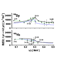
Figure 10: (Color online) Reduced transition probabilities $B(E2;I\,yr\,\rightarrow\,I-2\,yr)$ along the yrast line. Experimental data (filled squares) are connected with a thin line to guide eyes. The results of calculations by means of Eq.(66) and of Eq.(61) are connected by dashed and solid lines, respectively.

For illustrative purposes, to get a rough idea on the major trend of the quadrupole transitions, we employ the relations from the pairing-plus-quadrupole model (cf Ref.fra, )

$$m\omega_{0}^{2}\beta\,cos\gamma = \chi\langle Q_{0}\rangle$$

$$m\omega_{0}^{2}\beta\,sin\gamma =- \chi\langle Q_{2}\rangle$$ (62)

between the deformation parameters $\beta$ and $\gamma$ and two intrinsic quadrupole moments. By dint of Eq.(62) and the definition of the quadrupole isoscalar strength $\chi=4\pi m\omega^{2}_{0}/5\langle r^{2}\rangle\approx 4\pi m\omega^{2}_{0}/(3AR^{2})$ ($R\approx 1.2A^{\frac{1}{3}}fm$) one can express the $E2$-transition probability via the deformation parameters $\beta$ and $\gamma$

$$B(E2;\,I\,n_{w}=1\rightarrow I\pm 1\,yr)=\Theta\times$$ (63)

$$\frac{\beta^{2}}{\langle\hat{J}_{x}\rangle}\Biggl{[}\Biggl{(}\frac{W_{2}}{W_{3}}\Biggl{)}^{\frac{1}{4}}sin(\frac{\pi}{3}-\gamma)\pm\Biggl{(}\frac{W_{3}}{W_{2}}\Biggr{)}^{\frac{1}{4}}sin\gamma\Biggr{]}^{2}$$

where $\Theta=(9/16\pi^{2})e^{2}Z^{2}R^{4}$. Depending on the sign of $\gamma$-deformation (for $W_{2,3}>0$) one obtains selection rules for the quadrupole transitions from the one-phonon wobbling band to the yrast one

$$a) For\,-60^{o}<\gamma<0:$$

$$B(E2;I\,n_{w}\rightarrow I-1yr)>B(E2;I\,n_{w}\rightarrow I+1yr)$$

$$b) For\,0<\gamma<60^{o}:$$

$$B(E2;I\,n_{w}\rightarrow I+1yr)>B(E2;I\,n_{w}\rightarrow I-1yr)$$

For the intraband transitions we obtain

$$B(E2;\,I\,n_{w}\rightarrow I-2\,n_{w})=\frac{1}{2}\Theta\beta^{2}cos^{2}(\frac{\pi}{6}-\gamma)$$ (66)

One observes from Eq.(66) that for the transitions along the yrast line ($n_{w}=0$) the onset of the positive (negative) values of $\gamma$-deformation leads to the increase (decrease) of the transition probability along the yrast line.

Experimental values of $B(E2,\,I\,\nu\,\rightarrow\,I^{\prime}\,yr)$ are deduced from the half life of the yrast states nndc using the standard, long wave limit expressions $B(E2,i\,\rightarrow\,f)=\ P(i\,\rightarrow\,f)/(1.223\times 10^{9}E^{5}_{\gamma})\,\,(e^{2}$ fm${}^{4})$ RS . Here, the transition energy $E_{\gamma}$ is in MeV and the absolute transition probability $P(i\,\rightarrow\,f)=\ln 2/T(i\,\rightarrow\,f)$ is the related to the half life $T(i\,\rightarrow\,f)$ (in seconds). When comparing our results with experimental data, we take into account the Clebsh-Gordon coefficient (see Eq.(56)) up to $I\leq 10\hbar$. For $I>10\hbar$ the asymptotic value for the Clebsh-Gordon coefficient, which is 1, is used. Note that in the vicinity of the backbending the mean field description becomes less reliable (cf Ref.ikuko, ). While the cranking approach should be complemented with a projection technique in the backbending region due large fluctuations of the angular momentum (cf Ref.RS, ), its validity becomes much better at high spins. Evidently, the larger is the rotational frequency the stronger is a predictive power of the CRPA, since it is based on the cranking approach aimed for the high spin physics fra .

Experimental data for the quadrupole transitions along the yrast line are compared with the results of calculations: (a) by means of Eq.(61) and calculations (b) by means of Eq.(66) (see Fig.10). In the calculations (a) we use the mean field values for the quadrupole operators. The calculations (a) evidently manifest the backbending effect obtained for the moments of inertia (see Figs.5,6) at $\hbar\Omega_{c}\approx 0.25,\,0.3$ MeV for ¹⁶²Yb and ¹⁵⁶Dy, respectively. Thus, the use of the self-consistent expectation values $\langle\hat{Q}^{(E)}_{m}\rangle$ is crucial to reproduce the experimental behaviour of the yrast band decay. The calculations (b) (Eq.(66)) reproduce the experimental data with less accuracy, while providing the major trend of the transitions with the sign of $\gamma$-deformation. The agreement between calculated and experimental values of intraband $B(E2)$ transitions along the yrast line is especially good after the transition point.

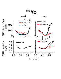
Figure 11: (Color online) ¹⁶²Yb. The electric B(E2)- (top) and the magnetic B(M1)- (bottom) reduced transition probabilities from the one-phonon bands to the yrast band. The positive (negative) signature phonon band is described by the first $r=+1$ ($r=-1$) RPA solution. One observes a strong dominance of the B(E2)- and B(M1)-transitions from the wobbling states ($r=-1$) with spin I to the yrast states with spin $I^{\prime}=I-1$, starting from the rotational frequency $\hbar\Omega>0.28$MeV. The transitions, calculated by means of the $\psi^{(\nu=1)}_{\mu}$ and $\phi^{(\nu=1)}_{\mu}$ phonon amplitudes, are connected by solid lines. On the right panels the results obtained by means of Eqs.(60), (73) (with the aid of the variables $W_{2,3}$, Eq.(44)) are connected by thin lines, starting from the rotational frequency $\hbar\Omega\approx 0.3$ MeV. This point is associated in our analysis with the appearance of wobbling excitations.

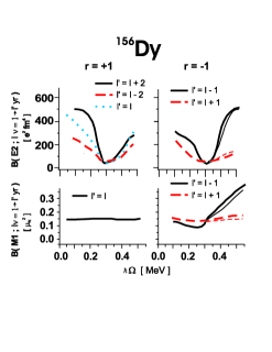
Figure 12: (Color online) ¹⁵⁶Dy. Similar to Fig.11. One observes a strong dominance of the B(E2)- and B(M1)-transitions from the wobbling states ($r=-1$) with spin I to the yrast states with spin $I^{\prime}=I-1$ starting from the rotational frequency $\hbar\Omega\geq 0.3$MeV.

At small rotational frequency, in the both nuclei, transitions probabilities from the first positive and negative signature RPA solutions are much weaker compare with the quadrupole transitions along the yrast line (see Fig.10 and top panels of Figs.11,12). At $\hbar\Omega\sim 0.05$MeV the transition strengths for the first positive ($r=+1$) and negative ($r=-1$) RPA solutions are : $\sim 330e^{2}fm^{4}$ for ¹⁶²Yb and $\sim 500e^{2}fm^{4}$ for ¹⁵⁶Dy, with small differences between different transitions due to the Clebsh-Gordon coefficients. On the other hand, we obtain a good correspondence between the shape evolution and the selection rules (III.5) for the both nuclei (see top panels of Figs.11,12 and Fig.2). The transition probabilities, Eq.(59), are calculated by means of the $\psi^{(\nu)}_{\mu}$ and $\phi^{(\nu)}_{\mu}$ phonon amplitudes expressed via the coordinate and momentum amplitudes (see Eqs.(15),(16),(17),(30)). We compare these results for the first negative signature RPA solution (which is associated with a wobbling mode) with the results obtained with the aid of the Marshalek moments of inertia (see Eqs.(38),(44),(60)). Evidently, if the ”spurious” solution (the redundant mode) is not removed from Eq.(19), it contributes to the variables (30). These variables can not obey to the condition (33) in this case. As a result, the orthogonality condition Eq.(27) is broken and Eqs.(59),(60) for the transitions should produce completely different results. A good agreement between the both calculations (see the right top panels in Figs.11,12) is the most valuable proof of the validity of our approach. The observed negligible differences are due the approximate fulfillment of the conservation laws (20), caused by the presence of the additional term (II.1) (see Fig.4).

According to our analysis, at $\hbar\Omega\sim 0.25$MeV there is a transition from the axially-deformed to nonaxial shapes with the negative $\gamma$-deformation in ¹⁶²Yb (see Fig.2 and the discussion in Ref.JK05, ). With a slight increase of the rotational frequency, starting from $\hbar\Omega\sim 0.28$MeV, the excited band of the negative signature, created by the first RPA solution, changes the decay properties. The negative values of $\gamma$-deformation produce the dominance of the inter-band quadrupole transitions from the one-phonon state to the yrast ones with a lower spin ($\Delta I=1$, the case Eq.(III.5), a)).

Similar results are obtained in ¹⁵⁶Dy for the lowest negative signature excited band, created by the first RPA solution. At low angular momenta ($\hbar\Omega\leq 0.3$MeV) this band populates with approximately equal probabilities the yrast states with $I^{\prime}=I\pm 1$ ($I$ is the angular momentum of the excited state). At $\hbar\Omega\sim 0.3$MeV a shape-phase transition occurs, that leads to the triaxial shapes with the negative $\gamma$-deformation. In turn, the excited band, created by the first RPA solution, decays stronger on the yrast states with angular momenta $I^{\prime}=I-1$ ($\Delta I=1$, the case Eq.(III.5), a)), starting from $\hbar\Omega\geq 0.32$MeV.

From the above analysis of the electric quadrupole transitions one notices that there is no need to know the definition of the wobbling phonon operator in the UR frame. Indeed, in this frame the direction of the angular momentum is fixed and fluctuations of the angular momentum are absent. However, there is a vibrational mode, related to the shape fluctuations, that carries one unit of the angular momentum. According to Bohr and Mottelson consideration, in the PA frame the system shape is fixed, while the angular momentum fluctuates around the rotation axis that coincides with one of the principal axes of the inertia tensor. Evidently, the result for the transition probabilities in the lab frame must be independent on the the choice of the reference frame.

To prove the equivalence of the both results for the electric quadrupole transitions, let us use the Bohr-Mottelson definition of the wobbling phonon operator, Eq.(A.5),

$${\hat{Q}}_{w}^{\dagger}=\frac{i}{\sqrt{2\langle{\hat{J}}_{x}\rangle}}\Biggl{[}(\hat{I}_{2})_{PA}\Biggl{(}\frac{W_{2}}{W_{3}}\Biggl{)}^{\frac{1}{4}}+(i\hat{I}_{3})_{PA}\Biggl{(}\frac{W_{3}}{W_{2}}\Biggl{)}^{\frac{1}{4}}\Biggr{]}.$$ (67)

Here, the quantities $W_{2,3}$ are determined by the Marshalek moments of inertia, Eqs.(44). In the PA frame one has to use the transformation Eq.(A.12) in order to calculate the transition probability and commutation relations Eq.(A.2). This transformation and the definition (67) yield the expression

$$B(E2;I\,w\,\rightarrow\,I\pm 1yr)=\left|\langle\left[\hat{M}_{2\mu_{1}=\pm 1}^{(E)},\hat{O}_{w}^{\dagger}\right]\rangle\right|^{2}=$$

$$\frac{1}{4\langle{\hat{J}}_{x}\rangle}\Biggl{|}\left(\frac{W_{2}}{W_{3}}\right)^{\frac{1}{4}}A^{(E)}\mp\left(\frac{W_{3}}{W_{2}}\right)^{\frac{1}{4}}B^{(E)}\Biggr{|}^{2}$$ (68)

that is similar to Eq.(60), obtained in the UR frame, indeed. We will use this fact below to understand major features of the magnetic transitions from the wobbling band.

In the CRPA approach the magnetic transitions are defined as

$$B(M1;I\,\nu\rightarrow\,I\pm 1\,yr)\approx\left|\langle\left[\hat{M}_{1\mu_{1}=\pm 1}^{(M)},\hat{O}_{\nu}^{\dagger}\right]\rangle\right|^{2}$$ (69)

With the aid of the transformation from x-to z-axis quantization Eq.(58) one obtains

$$B(M1;I\,\nu\rightarrow\,I\pm 1\,yr)\approx\frac{1}{2}\left|i\left[{\hat{M}}^{(M)}_{1\nu_{3}=1},{\hat{O}}_{\nu}^{\dagger}\right]\mp\left[{\hat{M}}^{(M)}_{1\nu_{3}=0},{\hat{O}}_{\nu}^{\dagger}\right]\right|^{2}$$ (70)

The linear boson term of the magnetic operator has a form (see also Ref.JK, )

$$\hat{M}^{(M)}_{1\nu_{3}=0,1}=\mu_{N}\sqrt{3}\left(\frac{1}{2}g_{s}^{(eff)}\hat{S}_{01\nu_{3}}+g_{l}^{(eff)}\hat{L}_{01\nu_{3}}\right)$$

$$=\frac{i^{\nu_{3}+2}}{2}\sum_{\mu}\Lambda^{(\nu_{3})}_{\mu}(b^{+}_{\mu}+(-1)^{\nu_{3}}b_{\mu}),$$ (71)

where $\mu_{N}$ is the nucleon magnetons, $g_{s}^{(eff)}$, $g_{l}^{(eff)}$ are the spin and orbital effective gyromagnetic ratios, respectively; and the quasiparticle matrix elements $\Lambda^{(\nu_{3})}_{\mu}$ are real. Taking into account the definition of the phonon operator Eq.(15), we express the magnetic transition with the aid of generalized coordinate and momentum amplitudes Eqs.(16)

$$B(M1;I\,\nu\rightarrow\,I\pm 1\,yr)\approx\left|\sum_{\mu}\Lambda^{(1)}_{\mu}X_{\mu}^{\nu}\mp\sum_{\mu}\Lambda^{(0)}_{\mu}P_{\mu}^{\nu}\right|^{2}$$ (72)

Are there any specific features of magnetic transitions from the wobbling band, related to the sign of $\gamma$-deformation ? Our results evidently demonstrate the dominance of $B(M1;I\,n_{W}\rightarrow I-1yr)$ (see the right bottom panels in Figs.11,12) for the both nuclei. To get an insight of this result, we define the magnetic transitions by dint of the Marshalek moments of inertia. With aid of the definition, Eq.(67), the transformation, Eq.(A.12), and commutation relations $[\hat{I}_{1}\pm i\hat{I}_{2},\hat{M}_{\lambda m}]=\sqrt{\lambda(\lambda+1)-m(m\mp 1)}\hat{M}_{\lambda m\mp 1}$ for the PA frame BM1 , we obtain from Eq.(69)

$$B(M1;I\,\nu\,\rightarrow\,I\pm 1\,yr)\approx\biggl{|}\langle\hat{M}^{(M)}_{1\nu_{3}=1}[r=+1]\rangle\biggr{|}^{2}\times$$

$$\times\frac{1}{4\langle{\hat{J}}_{x}\rangle}\frac{(\sqrt{W_{3}}\mp\sqrt{W_{2}})^{2}}{\sqrt{W_{2}W_{3}}}$$ (73)

Although the expression for the magnetic transitions, Eq.(73), is similar to the one of the Bohr-Mottelson model, we stress that the moments of inertia are defined self-consistently within the CRPA approach. Notice that the dipole magnetic moment $\langle\hat{M}^{(M)}_{1\nu_{3}=1}[+]\rangle$ increases quite drastically, if a nucleus is undergoing the backbending (see the discussion about $M1$ strength in Ref.JK2, ). Keeping in mind that for the wobbling states $W_{2,3}>0$, we have

$$B(M1;I\,n_{W}\rightarrow I-1yr)>B(M1;I\,n_{W}\rightarrow I+1yr)$$ (74)

Thus, the tendency observed in the microscopic calculations with the aid of the phonon amplitudes are understood in terms of the rules Eq.(74). Independently on the sign of the $\gamma$-deformation of rotating nonaxial nuclei, these rules determine the dominance of $\Delta I=1\hbar$ magnetic transitions from the wobbling to the yrast states.

IV Summary

The observation of the wobbling excitations among excited states near the yrast line is one of the most convincing manifestations of the nonaxial deformation in rotating nuclei. In this paper we present a transparent, self-consistent derivation of the basic equations for the wobbling excitations in the UR (time-independent) frame, that determine: i) the energy spectrum and ii)electromagnetic properties of these states in even-even nuclei. We obtained the same expressions for the effective moments of inertia (38) as those obtained by Marshalek in the time-dependent Hartree-Bogoliubov approach in the PA frame mar2 . We established one-to-one correspondence between the main characteristics of the wobbling excitations in the Bohr-Mottelson model and those that are derived within the CRPA approach. Note, however, that the CRPA breaks down at the transition point when $\Delta_{p}$ or $\Delta_{n}$ vanish mar1 . We have avoided this problem by means of the phenomenological prescription for the rotational dependence of the pairing gap. A good agreement between the dynamic moment of inertia calculated at the mean field approximation and the Thouless-Valatin moment of inertia calculated in the RPA supports the consistency of our mean field calculations (see Fig.3). In contrast to the standard RPA calculations, where the residual strength constants are fixed for all values of $\Omega$ (see e.g. shi1 ; mat1 ; mat2 ), we determine the strength constants for each value of $\Omega$ by the requirement of the validity of the conservation laws. This enables us to overcome the instability of the RPA calculations at the transition region, at least, for the excitations. In principle, projection methods may be used in the transition region in order to calculate transition matrix elements. Although the amplitudes $\phi^{(\nu)}_{\mu}$ (see Eq.(15)) are higher for the RPA modes in the transition region than in other regions, the relation $|\phi^{(\nu)}_{\mu}|<|\psi^{(\nu)}_{\mu}|$ is still valid to hold the QBA. And least but not last, the CRPA becomes quite effective at high spins, after the transition point, when the pairing correlations still persist.

From our analysis it follows that an excited band can be considered as the wobbling one, if the magnetic transitions from this band into the yrast one fulfil the condition Eq.(74). Note that these rules do not depend on the sign of $\gamma$-deformation. In contrast, the electric quadrupole transitions from this band to the yrast one must fulfil the staggering rules Eq.(III.5) depending on the sign of $\gamma$-deformation. The transition from this band are characterised by a high collectivity. We predict that the lowest excited negative signature and positive parity band in ¹⁶²Yb (which is a natural prolongation of the odd angular momentum part of the $\gamma$-band) transforms to the wobbling band at $\hbar\Omega>0.3$MeV. We found that strong E2 transitions from this band populate the yrast states, with the branching ratio $B(E2;I\,w\,\rightarrow\,I-1yr)/B(E2;I\,w\,\rightarrow\,I+1yr)>1$. Such a behaviour is brought about by the onset of nonaxial nuclear shapes with the negative sign of $\gamma$-deformation after the backbending. According to our definition of $\gamma$-deformation, with the increase of the rotational frequency the system is driving to a noncollective oblate rotation (around the x-axes). This trend is confirmed by a good agreement between the results for the quadrupole transitions along the yrast line and available experimantal data (see Fig.10). Similar transition occurs in ¹⁵⁶Dy after the backbending as well, at $\hbar\Omega>0.3$MeV. In this nucleus we found that the lowest negative signature and positive parity band represents a natural prolongation of the $\gamma$-band with odd spins, observed at small angular momenta up to $\hbar\Omega\sim 0.3$MeV. At rotational frequency $\hbar\Omega>0.3$MeV this band created by the first RPA solution transforms to the wobbling excitations. A good agreement between calculated in the CRPA and experimental Routhians allows us to conclude that the experimental states, associated with $(+,1)_{1}$ band in Ref.Kon, , are wobbling excitations at the rotational frequency values $0.45$MeV$<\hbar\Omega<0.55$MeV. These states fulfil all requirements that are specific for the wobbling excitations of nonaxially deformed rotating nuclei, with the negative $\gamma$-deformation. Evidently, it is quite desirable to obtain new experimental data on electromagnetic decay properties of these states in order to reach a final conclusion about our prediction and, respectively, on the validity of the CRPA analysis.

Appendix A Asymmetric rotor model

In this appendix we review the basic features of the wobbling excitations in the rotor model BM75 in order to compare with the microscopic model discussed in section III. In addition to well known results, we provide a novel analysis of magnetic properties of the wobbling states.

At high-spin limit $I>>1$, the rotor Hamiltonian has the following form (see Ref.BM75, )

$$\hat{H}=\hat{H}_{0}+\frac{\hbar^{2}}{2\Im_{1}}(\hat{I})^{2}_{PA}+\hat{H}_{wobb}$$ (A.1)

$$[\hat{I}_{i},\hat{I}_{j}]_{PA}=-i\varepsilon_{ijk}(\hat{I}_{k})_{PA}$$ (A.2)

where $(\hat{I}_{i})^{2}_{PA}$ and $\Im_{i}$ are the angular momentum and principal moment of inertia components in the rotating, principal axis (PA) coordinate system. It is assumed that the yrast band is generated by rotation around the x-axis $I\approx I_{1}=K$. Small oscillations of the angular momentum create wobbling excitations described by the term

$$\hat{H}_{wobbl} = \hbar\,\omega_{w}\,\,\left(\hat{Q}_{wobb}^{+}\hat{Q}_{wobb}\,+\,\frac{1}{2}\right)$$

$$\hbar\omega_{w} = \hbar^{2}I\sqrt{W_{2}W_{3}}$$ (A.3)

where

$$W_{2}=\frac{1}{\Im_{2}}\,-\,\frac{1}{\Im_{1}}\,,\qquad W_{3}=\frac{1}{\Im_{3}}\,-\,\frac{1}{\Im_{1}}$$ (A.4)

The wobbling (excited) state at spin $I$ is created by the wobbling phonon

$$\hat{O}^{+}_{wobb}=xB^{+}-yB\,\Leftrightarrow\,B^{+}=x\hat{O}^{+}_{wobbl}+y\hat{O}_{wobbl}$$ (A.5)

with

$$B^{+} = \frac{i}{\sqrt{2I}}(\hat{I}_{2}+i\hat{I}_{3})_{PA},\quad B=(B^{+})^{+},$$ (A.6)

$$x = \frac{\sqrt{W_{3}}+\sqrt{W_{2}}}{2}(W_{2}W_{3})^{-1/4}$$ (A.7)

$$y = \frac{\sqrt{W_{2}}-\sqrt{W_{3}}}{2}(W_{2}W_{3})^{-1/4}$$ (A.8)

and a normalization condition $x^{2}-y^{2}=1$. From Eq.(A.3) it follows that the diagonalization of $\hat{H}_{wobb}$ requires $W_{2}>0$, $W_{3}>0$ and $\Im_{1}>\Im_{2}>\Im_{3}$.

At $(I\approx I_{1}>>0)$ the eigenfunction of Hamiltonian (A.1) is a product of the Wigner $\cal D$ - function and the intrinsic eigenfunction defined by the wobbling quantum number $|n_{w}\rangle=(Q^{+}_{wobb})^{n_{w}}~{}|0\rangle$. The variable $n_{w}$

$$n_{w}=\langle IK|B^{+}B|IK\rangle\approx I-I_{1}=I-K$$ (A.9)

is defined with respect to the state $|IK=(I_{1})_{PA}\rangle\equiv|n_{w}\rangle$ such that $B^{+}|IK\rangle=\sqrt{n_{w}+1}|IK-1\rangle=\sqrt{n_{w}+1}|n_{w}+1\rangle$ and $|0\rangle=|IK=I\rangle$. The transition probability for the operator of type $X$ and multipolarity $\lambda$

$$B(X\lambda;I\nu K_{\nu}\rightarrow I^{\prime}\nu^{\prime}K_{\nu}^{\prime})=$$

$$\frac{1}{2I+1}\,\,|\langle I^{\prime}K^{\prime}_{\nu}\nu^{\prime}||\hat{\cal M}(X\lambda)||IK_{\nu}\nu\rangle|^{2}$$ (A.10)

is defined by the reduced matrix element

$$\langle I^{\prime}K^{\prime}n_{w}^{\prime}||\hat{\cal M}(X\lambda)||IKn_{w}\rangle=\sqrt{2I+1}\times$$ (A.11)

$$\sum^{\lambda}_{\nu_{1}=-\lambda}\langle n_{w}^{\prime}|(IK\lambda\nu_{1}|I^{\prime}K^{\prime})\hat{\cal M}(X\lambda\nu_{1}=I^{\prime}-I)|n_{w}\rangle$$

Notice that the eigenmodes of the Hamiltonian $\hat{H}_{0}$ do not change the projection $K$ onto the first PA axis. However, if the wobbling mode is excited with $|n_{w}^{\prime}-n_{w}|\neq 0$, the projection $K$ is changed and corresponding Clebsch-Gordan coefficients in Eq.(A.11) can be expressed in terms of $B^{+}$, $B$ operators (see Section 4.5c in Ref.BM75, ).

Using this procedure for the Clebsch-Gordan coefficients, a relation between multipole operators in the PA frame with the x- and z-quantization axis and the definition Eq.(10)

$${\hat{\cal M}}(X\lambda\mu_{1})=\sum_{\mu_{3}}\,\,{\cal D}^{\lambda}_{\mu_{1}\mu_{3}}(0,\frac{\pi}{2},0)\,\,{\hat{\cal M}}(X\lambda\mu_{3}),$$ (A.12)

we obtain for interband E2 transitions between the one-phonon wobbling band ($n_{w}=1$) and the yrast band ($n_{w}=0$)

$$B(E2;\,I\,n_{w}\rightarrow I\pm 1\,yr)=|\varrho_{1}A^{(E)}\mp\varrho_{2}B^{(E)}|^{2}$$ (A.13)

Here, the variables $A^{(E)}$ and $B^{(E)}$ are defined by Eqs.(25), (26), $\hat{Q}^{(E)}_{m}\equiv e\frac{Z}{A}\hat{Q}_{m}$ and

$$\varrho_{1}=\frac{1}{\sqrt{2I}}\left(\frac{W_{2}}{W_{3}}\right)^{\frac{1}{4}},\quad\varrho_{2}=\frac{1}{\sqrt{2I}}\left(\frac{W_{3}}{W_{2}}\right)^{\frac{1}{4}}$$ (A.14)

For intraband transitions we have

$$B(E2;\,I\,n_{w}\rightarrow I-2\,n_{w})=\frac{1}{8}\left|\sqrt{3}\langle\hat{Q}^{(E)}_{0}\rangle-\langle\hat{Q}^{(E)}_{2}\rangle\right|^{2}$$ (A.15)

Here, we use the fact that $\langle\hat{\cal M}(E2,\nu_{1}=\pm 1)\rangle=0$ and $\langle\hat{\cal M}(E2,\nu_{1}=2)\rangle=\langle\hat{\cal M}(E2,\nu_{1}=-2)\rangle$ and neglect terms of order or higher than $\sim\frac{1}{I}$.

Similar procedure, described above, can be employed to derive M1 transitions from one-phonon wobbling band into the yrast band. Ignoring the terms of order $I^{-1}$ in Eq.(A.11) at high-spin limit ($I\approx K>>1$), we have the following approximative values for the Clebsch-Gordan coefficients in terms of the matrix elements of the operators $B$, $B^{+}$ (or $\hat{Q}_{wobb}$, $\hat{Q}^{+}_{wobb}$)

$$(I\,K\,1\,0\,|\,I\,K) \rightarrow \,\,1$$

$$(I\,K\,1\,0\,|\,I\pm 1\,K) \rightarrow \pm\frac{1}{\sqrt{I}}\langle n\pm 1|\begin{array}[]{c}B^{+}\\ B\end{array}|n\rangle$$ (A.18)

$$(I\,K\,1\,\pm 1\,|\,I\,K\pm 1) \rightarrow \mp\frac{1}{\sqrt{I}}\langle n\mp 1|\begin{array}[]{c}B\\ B^{+}\end{array}|n\rangle$$ (A.21)

$$(I\,K\,1\,\pm 1\,|\,I\pm 1\,K\pm 1) \rightarrow 1$$ (A.22)

Since $\langle\hat{\cal M}(M1\,\nu_{1}=\pm 1)\rangle=0$, we obtain

$$\langle I^{\prime}K^{\prime}n_{w}^{\prime}||\hat{\cal M}(M1\,\nu_{1}=0)||IKn_{w}\rangle=$$

$$\sqrt{2I+1}\langle n^{\prime}_{w}|\Biggl{[}\delta_{I^{\prime},I}\langle\hat{\cal M}(M1,\nu_{1}=0)\rangle+$$

$$+ \,\delta_{I^{\prime},I+1}\frac{1}{\sqrt{I}}\langle\hat{\cal M}(M1,\nu_{1}=0)\rangle\,(x\hat{Q}^{+}_{wobb}+y\hat{Q}_{wobb})$$

$$- \delta_{I^{\prime},I-1}\frac{1}{\sqrt{I}}\langle\hat{\cal M}(M1,\nu_{1}=0)\rangle\,(x\hat{Q}_{wobb}+y\hat{Q}^{+}_{wobb})\Biggr{]}|n_{w}\rangle$$

Here, ${\hat{\cal M}}(M1;\nu_{1})=\mu_{N}\,\sqrt{3}\sum_{i=1}^{A}$ $($ $\frac{1}{2}g_{s}^{(i,eff)}[\sigma\otimes Y_{l=0}]_{1\nu_{1}}\,+\,$ $g_{l}^{(i,eff)}[l\otimes Y_{l=0}]_{1\nu_{1}}$ $)$ is a magnetic dipole operator. With the aid of Eqs.(A.7), (A.8),(A.12) and the definition of operators given in Ref.JK, , we obtain for M1 transitions from the one-phonon wobbling band ($n_{w}=1$) into the yrast band ($n_{w}=0$) the following expression

$$B( M1 ;I\,n_{w}\rightarrow I\pm 1yr)=\biggl{|}\langle\hat{M}^{(M)}_{1\nu_{3}=1}[r=+1]\rangle\biggr{|}^{2}\times$$ (A.24)

$$\times\frac{1}{4I}\frac{(\sqrt{W_{3}}\mp\sqrt{W_{2}})^{2}}{\sqrt{W_{2}W_{3}}}$$

The magnetic moment $\langle\hat{M}^{(M)}_{1\nu_{3}=1}[+]\rangle$ can be calculated in any microscopic model.

References

- (1) A. Bohr and B. R. Mottelson, Nuclear Structure Vol. II (Benjamin, New York, 1975).
- (2) S. G. Nilsson and I. Ragnarsson, Shapes and Shells in Nuclear Structure (Cambridge University Press, Cambridge, 1995).
- (3) P. G. Reinhard, V. O. Nesterenko, E. Suraud, S. El Gammal, and W. Kleinig, Phys. Rev. A 66, 013206 (2002).
- (4) see I. Bialynicki-Birula and T. Sowinski, Phys. Rev. A 71, 043610 (2005) and references therein.
- (5) D. Janssen and I. N. Mikhailov, Nucl. Phys. A318, 390 (1979).
- (6) E. R. Marshalek, Nucl. Phys. A331, 429 (1979).
- (7) S. W. Ødegård et al., Phys. Rev. Lett. 86, 5866 (2001); D. R. Jensen et al., Phys. Rev. Lett. 89, 142503 (2002), Nucl. Phys. A703, 3 (2002); H. Amro et al., Phys. Lett. B 553, 197 (2003); G. Schönwasser et al., Phys. Lett. B 552, 9 (2003); A. Görgen et al., Phys. Rev. C 69, 031301(R) (2004); D. R. Jensen et al., Eur. Phys. J. A 19, 173 (2004).
- (8) S. Frauendorf, Rev. Mod. Phys. 73, 463 (2001).
- (9) A. Johnson, H. Ryde, and J. Sztarkier, Phys. Lett. B 34, 605 (1971).
- (10) S. Frauendorf and F. R. May, Phys. Lett. B 125, 245 (1983).
- (11) P. H. Regan et al., Phys. Rev. Lett. 90, 152502 (2003).
- (12) J. Kvasil and R. G. Nazmitdinov, Phys. Rev. C 69, 031304(R) (2004); J. Kvasil, R. G. Nazmitdinov, and A. S. Sitdikov, Physics of Atomic Nuclei 97, 1650 (2004).
- (13) J. Kvasil and R. G. Nazmitdinov, Pis’ma v ZhETF, 83, 227 (2006) (JETP Lett. 83, 187 (2006)); Phys. Rev. C 73, 014312 (2006).
- (14) I. N. Mikhailov and D. Janssen, Phys. Lett. B 72, 303 (1978).
- (15) D. Janssen, I. N. Mikhailov, R. G. Nazmitdinov, B. Nerlo–Pomorska, K. Pomorski, and R. Kh. Safarov, Phys. Lett. B 79, 347 (1978).
- (16) Y. R. Shimizu and M. Matsuzaki, Nucl. Phys. A 588, 559 (1995).
- (17) I. Hamamoto, Phys. Rev. C 65, 044305 (2002).
- (18) I. Hamamoto and G. B. Hagemann, Phys. Rev. C 67, 014319 (2003).
- (19) M. Matsuzaki, Y. R. Shimizu, and K. Matsuyanagi, Phys. Rev. C 65, 041303(R) (2002).
- (20) M. Matsuzaki, Y. R. Shimizu, and K. Matsuyanagi, Phys. Rev. C 69, 034325 (2004).
- (21) J. Kvasil, N. Lo Iudice, R. G. Nazmitdinov, A. Porrino, and F. Knapp, Phys. Rev. C 69, 064308 (2004).
- (22) H. Sakamoto and T. Kishimoto, Nucl. Phys. A 501, 205 (1989).
- (23) R. F. Casten, E. A. McCutchan, N. V. Zamfir, C. W. Beausang, and Jing-ye Zhang, Phys. Rev. C 67, 064306 (2003).
- (24) T. Nakatsukasa, K. Matsuyanagi, S. Mizutori, and Y. R. Shimizu, Phys. Rev. C 53, 2213 (1996).
- (25) J. Kvasil and R. G. Nazmitdinov, Fiz. Elem. Chastits At. Yadra 17, 613 (1986) [Sov. J. Part. Nucl. 17, 265 (1986)].
- (26) J. Kvasil, N. Lo Iudice, V. O. Nesterenko, and M. Kopál, Phys. Rev. C 58, 209 (1998).
- (27) F. G. Kondev et al., Phys. Lett. B 437, 35 (1998).
- (28) R. Wyss, W. Satula, W. Nazarewicz and A. Johnson, Nucl. Phys. A 511, 324 (1990).
- (29) R. G. Nazmitdinov, D. Almehed, and F. Dönau, Phys. Rev. C 65, 041307(R) (2002).
- (30) P. Ring and P. Schuck, The Nuclear Many-Body Problem (Springer-Verlag, New York, 1980).
- (31) E. R. Marshalek, Nucl. Phys. A 275, 416 (1977).
- (32) D. A. Varshalovich, A. N. Moskalev, and V. K. Khersonskii, Quantum theory of Angular Momentum (World Scientific, Singapore, 1986 ).
- (33) D. Almehed, F. Dönau, and R. G. Nazmitdinov, J. Phys. G: Nucl. Part. Phys. 29 2193 (2003).
- (34) http://www.nndc.bnl.gov/nudat2/
- (35) I. Hamamoto, Nucl. Phys. A 271, 15 (1976).
- (36) R. G. Nazmitdinov, Yad. Fiz. 46, 732 (1987) [ Sov. J. Nucl. Phys. 46, 412 (1987)].
- (37) E. R. Marshalek, Nucl. Phys. A 266, 317 (1976).
- (38) A. Bohr and B. R. Mottelson, Nuclear Structure Vol. I (Benjamin, New York, 1969).