Abstract

Medium modification of pion form factor has been evaluated in asymmetric nuclear matter (ANM). It is shown that both the shape and the pole position of the pion form factor in dense asymmetric nuclear matter is different from its vacuum counterpart with $\rho$-$\omega$ mixing. This is due to the density and asymmetry dependent $\rho$-$\omega$ mixing which could even dominate over its vacuum counterpart in matter. Results are presented for arbitrarily mixing angle. Effect of the in-medium pion factor on experimental observables e.g., invariant mass distribution of lepton pairs has been demonstrated.

25.75.Dw; 21.65.+f; 14.40.-n

1 Introduction

The pion electromagnetic form factor, $F_{\pi}(Q^{2})$ in vacuum shows that the physical $\rho$ meson is not a pure isospin eigenstate and it can mix with the $\omega$ meson [1]. In vacuum this mixing amplitude can be determined by measuring $F_{\pi}(Q^{2})$ which, although dominated by the $\rho^{0}$ pole, shows a kink near the $\omega$ meson mass. Such mixing (after electromagnetic correction) implies that the charge symmetry is broken at the most fundamental level in strong interaction through the small mass difference between up and down quarks in the QCD Lagrangian. Consequently, the physical $\rho$ and $\omega$ mesons that we deal with are admixtures of the corresponding isospin eigenstates. At the hadronic level this mixing can be understood in terms of neutron-proton mass difference in effective models [2].

$\rho$-$\omega$ mixing has important and interesting consequences. It plays a crucial role in generating contributions to few body charge symmetry violating observables [3]. The $\rho$-$\omega$ mixing amplitude is determined from $e^{+}e^{-}\rightarrow\pi^{+}\pi^{-}$ by measuring the pion form factor in the interference region [1]. With the extracted value of the mixing amplitude one is able to explain a number of observables namely, the non-Coulombic binding energy difference (Nolen Schiffer anomaly [4, 5]) of $A=3$ (mirror) nuclei, significant contributions to the $np$ asymmetry at 183 MeV and non-negligible contributions to the difference of $nn$ and $pp$ scattering lengths [6].

The mixing of different isospin states will be modified in matter. Such medium effects have recently been investigated by several authors [7, 8, 9]. Unlike neutron-proton mass difference, which is responsible for $\rho$-$\omega$ mixing in free space, the mixing in matter can be induced if the neutron-proton densities are different. This happens even if the Hamiltonian preserves the isospin symmetry i. e., if $M_{n}=M_{p}$, akin to the ‘spontaneous symmetry breaking’ driven by the $n\leftrightarrow p$ asymmetric ground state. It has been shown in Ref.[7] that the density dependent mixing is of similar magnitude as the usual vacuum mixing at normal nuclear matter density. Subsequently, Broniowski and Florkowski, showed that the mixing could be significantly large in $Pb$ like nuclei [8]. These studies were limited to hadronic models. In contrast, such density dependent $\rho$-$\omega$ mixing was studied within the framework of QCD sum-rule in Ref. [10] with similar results and conclusions. The sum rule calculation has recently been improved and extended to study the density dependent $\rho$-$\omega$ amplitude and its observable implications in heavy ion collisions [11].

In the present paper we revisit the problem within the framework of Walecka model [12]. We discuss the possible consequences in presence of a scalar mean field, an effective way to incorporate nucleon-nucleon interactions. Moreover, as in dense matter with large neutron-proton density asymmetry, the mixing angle could be quite high, we present results valid for arbitrary mixing angles. As an application, the possible modification of pion form factor in ANM and the $\pi^{+}\pi^{-}\rightarrow e^{+}e^{-}$ annihilation cross section at various densities and asymmetries have also been discussed. This is relevant for the dilepton production in relativistic heavy ion collisions. Therefore, the present investigation has direct relevance for the study of compressed baryonic matter (CBM) expected to be produced in heavy ion collisions at GSI energies [13].

Apart from $\rho-\omega$ mixing in asymmetric matter $\rho$ can also mix with the $\sigma$ in the same way as $\omega-\sigma$ mixing [14]. We have discussed such a possibility in Appendix I where it is argued that for matter with small neutron-proton asymmetry such possibilities could be ignored.

The paper is organized as follows. In the next section the formalism is set forth. In section 3 the relations between dilepton production cross section and form factor with mixing has been presented. Results are discussed in section 4 while section 5 is devoted to summary. Mathematical expressions relevant for the calculation of pion form factor with matter induced mixing and $\rho$ and $\omega$ meson self energies in dense nuclear matter are relegated to the appendix.

2 Formalism

The Lagrangian describing $\rho$ - $\omega$ meson-nucleon interaction is given by,

$${\cal L} = \bar{\psi}(\tau_{a}\Gamma_{a,\mu}\rho^{\mu}_{a})\psi+\bar{\psi}(\Gamma_{\omega,\mu}\omega^{\mu})\psi,$$

$$\Gamma_{v,\mu} = g_{v}\left[\gamma_{\mu}-\frac{\kappa_{v}}{2{\bar{M}}}\sigma_{\mu\nu}\partial^{\nu}\right].$$ (1)

Here ${\bar{M}}=(M_{p}+M_{n})/2$ where the subscript $p$ ($n$) stands for proton (neutron). Clearly, due to the Pauli matrix $\tau_{3}$, $\rho$ meson couples to neutron with a negative sign in contrast to the $\omega$ meson while with proton both couple with the same sign. This gives rise to mixing that vanishes in the limit, $M_{n}=M_{p}$ which is illustrated in Fig.1.

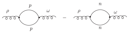
Figure 1: $\rho$ and $\omega$ nucleon loop

Here the mixing is generated by $N\bar{N}$ loop. The vacuum $\rho$-$\omega$ mixing in this approach was first calculated in Ref.[2]. We calculate similar mixing in ANM which, besides $n$-$p$ mass difference, would also depend both on baryon density $(\rho_{B})$ and the asymmetry parameter $\alpha=(\rho_{n}-\rho_{p})/(\rho_{n}+\rho_{p})$.

To determine the density and asymmetry dependent mixing amplitude we evaluate these loops at finite density which are characterized by the following density dependent polarization functions :

$$\Pi_{\mu\nu}^{\alpha\beta}=\frac{-i}{(2\pi)^{4}}\int{d^{4}}K~{}{\rm Tr}[i\Gamma^{\alpha}_{\mu}iG(K+Q){i\bar{\Gamma}^{\beta}_{\nu}}iG(K)]$$ (2)

where,

$$G(K)=G_{F}(K)+G_{D}(K)$$ (3)

$$G_{F}(K)=(K_{\mu}\gamma^{\mu}+M^{\ast})[\frac{1}{K^{2}-M^{\ast 2}+i\epsilon}]$$ (4)

$$G_{D}(K)=(K_{\mu}\gamma^{\mu}+M^{\ast})[\frac{i\pi}{E_{k}^{\ast}}\\ \delta(k_{0}-E_{k}^{\ast})\theta(k_{F}-|\vec{k}|)]$$

Here $G_{F}$ denotes free nucleon propagator while $G_{D}$ represents the density dependent part which forbids on mass shell nucleon propagation in matter due to Pauli blocking [12]. As the propagator now explicitly involves the Fermi momentum, contributions will be different for the neutron and proton loops if their densities (and hence Fermi momenta) are different. It is to be noted that the polarization function or the mixing amplitude will have two parts, one is like the polarization tensor with the free nucleon mass replaced by its effective mass called the free part representing nucleon-antinucleon excitations (Dirac sea) and the other one is density dependent part relevant for the scattering from the Fermi sphere. We discuss them separately.

2.1 Density dependent part

The density dependent piece of the mixed polarization ($\rho$-$\omega$) due to $p$-$p$ or $n$-$n$ excitations is generically given by

$$\Pi^{D}_{\mu\nu}(k_{F},M^{*},q_{0},|q|) = \frac{g_{\rho}g_{\omega}\pi}{(2\pi)^{4}}\int\frac{{d^{4}}K}{E_{k}^{\ast}}\delta(k^{0}-E_{k}^{\ast})$$ (5)

$$\theta(k_{F}-\mid\vec{k}\mid)\times\left[\frac{{\it{T}}_{\mu\nu}(K-Q,K)}{(K-Q)^{2}-M^{\ast 2}}\right.$$

$$\left.+\frac{{\it{T}}_{\mu\nu}(K,K+Q)}{(K+Q)^{2}-M^{\ast 2}}\right]$$

where $T_{\mu\nu}$ represents relevant traces as in Ref.[15].

The $\Pi_{\mu\nu}^{D}(q)=\Pi_{\mu\nu}^{vv}+\Pi_{\mu\nu}^{vt}$ functions in this case are as follows

$$\Pi_{\mu\nu}^{vv}(k_{F},M^{*},q_{0},|q|)=\frac{g_{\rho}g_{\omega}}{\pi^{3}}\int_{0}^{k_{F}}\frac{{d^{3}k}}{E_{k}^{\ast}}\frac{Q^{2}{\cal K}_{\mu\nu}-Q_{\mu\nu}(K\cdot Q)^{2}}{Q^{4}-4(K\cdot Q)^{2}}$$ (6)

$$\Pi_{\mu\nu}^{vt}(k_{F},M^{*},q_{0},|q|) = -\frac{g_{\rho}g_{\omega}}{\pi^{3}}(\frac{(k_{\rho})M^{\ast}}{8{\bar{M}}})2Q^{4}Q_{\mu\nu}$$ (7)

$$\times\int_{0}^{k_{F}}\frac{{d^{3}k}}{E_{k}^{\ast}}\frac{{1}}{Q^{4}-4(K\cdot Q)^{2}}$$

where ${\cal K}_{\mu\nu}=(K_{\mu}-\frac{K.Q}{Q^{2}}Q_{\mu})(K_{\nu}-\frac{K.Q}{Q^{2}}Q_{\nu})$, $Q_{\mu\nu}=(-g_{\mu\nu}+\frac{Q_{\mu}Q_{\nu}}{Q^{2}})$ and $E_{k}^{*}=\sqrt{k^{2}+M^{*2}}$. In the above expressions, for proton (neutron) loop we substitute $M$ and $k_{F}$ with $M_{p}$ ($M_{n}$) and $k_{F}^{p}$ ($k_{F}^{n})$ respectively. Moreover, at this point it might be recalled that for a vector meson moving in nuclear matter the longitudinal ($L$) transverse ($T$) polarization tensors are different because of ${\cal{K}}_{\mu\nu}$, unlike the vacuum part which is proportional to $Q_{\mu\nu}$. The $L$ and $T$ modes are constructed as $\Pi_{L}=-\Pi_{00}+\Pi_{33}$ and $\Pi_{T}=\Pi_{22}=\Pi_{11}$, where the meson momentum $Q=(q_{0},0,0,|q|)$ (see Appendix for details).

The mixing amplitude is characterized by $\Pi^{\rho\omega}_{L,T}$ which involves scattering from the neutron and proton Fermi spheres :

$$\Pi^{\rho\omega}_{L,T}=\Pi_{L,T}^{\rho\omega}(k_{F}^{p},M_{p}^{*},q_{0},|q|)-\Pi_{L,T}^{\rho\omega}(k_{F}^{n},M_{n}^{*},q_{0},|q|).$$ (8)

The negative sign arises because of the $\tau_{3}$ in the $\rho$-$NN$ interaction.

The pure part of the polarization can be obtained by taking appropriate vertex factor like $g_{\omega}$ or $g_{\rho}$ for both the vertices. Accordingly, the total is given by a sum over the neutron and proton loops instead of the difference.

$$\Pi^{\rho\rho}_{L,T}=\Pi_{L,T}^{\rho\rho}(k_{F}^{p},M_{p}^{*},q_{0},|q|)+\Pi_{L,T}^{\rho\rho}(k_{F}^{n},M_{n}^{*},q_{0},|q|)$$ (9)

and similarly $\rho\rightarrow\omega$ gives results for the $\omega$ meson polarization function. We take $g_{\omega}=10.1$, $\kappa_{\omega}=0$ and $g_{\rho}=2.63$, $\kappa_{\rho}=6.0$ [16] in numerical computations.

2.2 Free part

The vacuum part will also give rise to mixing which is same as Ref.[2] with $n$ and $p$ mass $M_{n,p}$ replaced by the in-medium masses, $M^{*}_{n,p}$. In Walecka model this is determined from the following self-consistent condition [12],

$$M_{n,p}^{*}=M_{n,p}-\frac{g_{\sigma}^{2}}{m_{\sigma}^{2}}(\rho_{p}^{s}+\rho_{n}^{s}),$$ (10)

where $\rho^{s}_{i}$ ($i=p,n$) represent scalar densities given by

$$\rho^{s}_{i}=\frac{M_{i}^{*}}{2\pi^{2}}\left[E^{*}_{i}k_{F}-M_{i}^{*2}\ln\left(\frac{E^{*}_{i}+k_{F}}{M_{i}^{*}}\right)\right].$$ (11)

The free part of the polarization tensor can be written as,

$$\Pi_{F}^{\mu\nu}=(-g^{\mu\nu}+Q^{\mu}Q^{\nu}/Q^{2})\Pi_{F}(Q^{2}).$$ (12)

The mixing contributions to $\Pi_{F}$ are given by :

$$\Pi_{F,vv}^{\rho\omega} = \frac{g_{\rho}g_{\omega}}{2\pi^{2}}\,Q^{2}\int_{0}^{1}\,dz\,z(1-z)\,\left[\ln\frac{M_{p}^{\ast 2}-Q^{2}\,z(1-z)}{{\bar{M}}^{2}-Q^{2}\,z(1-z)}\right.$$ (13)

$$\left.\frac{}{}-(p\rightarrow n)\right],$$

$$\Pi_{F,vt}^{\rho\omega} = \frac{g_{\rho}g_{\omega}}{2\pi^{2}}\,\frac{\kappa_{\rho}}{4}Q^{2}\left[\frac{M_{p}^{\ast}}{M_{p}}\int_{0}^{1}\,dz\ln\left\{\frac{M_{p}^{\ast 2}-Q^{2}\,z(1-z)}{{\bar{M}^{2}}-Q^{2}\,z(1-z)}\right\}\right.$$ (14)

$$\left.\frac{}{}-(p\rightarrow n)\right].$$

The pure $\rho$ ($\omega$) meson self-energies for the vector-vector, vector-tensor and tensor-tensor parts are given by [16]

$$\Pi_{F}^{\rho\rho(\omega\omega)} = \frac{g_{\rho(\omega)}^{2}}{2\pi^{2}}\,Q^{2}\sum_{i=p,n}\left[I_{1}^{(i)}\frac{}{}\right.$$ (15)

$$\left.+\frac{\kappa_{\rho(\omega)}}{2M_{i}}M_{i}^{\ast}I_{2}^{(i)}\right.$$

$$\left.+\frac{1}{2}\left(\frac{\kappa_{\rho(\omega)}}{2M_{i}}\right)^{2}(Q^{2}I_{1}^{(i)}+M_{i}^{\ast 2}I_{2}^{(i)})\right],$$

where

$$I_{1}^{(i)}=\int_{0}^{1}\,dz\,z(1-z)\,\ln\left[\frac{M_{i}^{\ast 2}-Q^{2}\,z(1-z)}{M_{i}^{2}-Q^{2}\,z(1-z)}\right],$$ (16)

$$I_{2}^{(i)}=\int_{0}^{1}\,dz\,\ln\left[\frac{M_{i}^{\ast 2}-Q^{2}\,z(1-z)}{M_{i}^{2}-Q^{2}\,z(1-z)}\right].$$ (17)

It is to be noted that the free part $\Pi^{\rho\omega}_{F}$ vanishes in the limit $M_{n}=M_{p}$. We extract the real part of the vacuum mixing amplitude (with free nucleon mass) to be $\sim-3447$MeV² at the omega pole and this is consistent with that of Ref. [17]. When in-medium nucleon masses are included $\Pi_{\rho\omega}^{F}(m_{\omega}^{2})$ is equal to $-3716$ MeV² and $-4675$ MeV² at $\rho_{0}$ and $2\rho_{0}$ respectively in symmetric nuclear matter.

3 Pion form factor and $\pi^{+}\pi^{-}\rightarrow{\mathrm{e}}^{+}{\mathrm{e}}^{-}$ cross section

The $\rho$-dominated (unmixed) pion electromagnetic form factor is given by:

$$F_{\pi}(Q^{2})=1-\frac{g_{\rho\pi\pi}}{g_{\rho}}\frac{Q^{2}}{Q^{2}-m_{\rho}^{2}+im_{\rho}\Gamma_{\rho}}$$ (18)

in the first form of VMD [1].

In presence of mixing, the above expression for pion form factor should be replaced by (see Appendix for detailed derivation)

$$F_{\pi}(Q^{2}) = 1-g_{\rho\pi\pi}\frac{s_{\omega}}{s_{\rho}s_{\omega}-\Pi_{\rho\omega}^{2}}\frac{Q^{2}}{g_{\rho}}-g_{\rho\pi\pi}\tan{\epsilon}$$ (19)

$$\times\frac{s_{\rho}}{s_{\rho}s_{\omega}-\Pi_{\rho\omega}^{2}}\frac{Q^{2}}{g_{\omega}}.$$

Here $\tan 2\epsilon=\frac{2\Pi_{\rho\omega}}{s_{\rho}-s_{\omega}}$ with $s_{\rho(\omega)}=Q^{2}-m_{\rho(\omega)}^{2}-\Pi_{\rho\rho(\omega\omega)}+im_{\rho(\omega)}\Gamma_{\rho(\omega)}$. Here the coupling of the physical $\rho$ and $\omega$ states to the photon is considered. In this form the $\omega\to\pi^{+}\pi^{-}$ decay is understood to proceed exactly like the $\rho$ but modified by the mixing factor $\tan\epsilon$ and $\Pi_{\rho\omega}^{2}$ as appears in the denominator.

In the small mixing limit the term quadratic in $\Pi_{\rho\omega}$ in Eq. 19 can be dropped and $\tan\epsilon\simeq\epsilon$. Thus, to lowest order in the mixing parameter $\epsilon$, the above expression takes the form [1]

$$F_{\pi}(Q^{2})=1-g_{\rho\pi\pi}\frac{1}{s_{\rho}}\frac{Q^{2}}{g_{\rho}}-g_{\rho\pi\pi}\,\epsilon\frac{1}{s_{\omega}}\frac{Q^{2}}{g_{\omega}}$$ (20)

The coupling constants used are $g_{\rho\pi\pi}^{2}/4\pi\sim 2.9$, $g_{\rho}^{2}/4\pi\sim 2.0$ [1] and

$$\frac{g_{\omega}}{g_{\rho}} = \sqrt{\frac{m_{\omega}\Gamma(\rho\rightarrow e^{+}e^{-})}{m_{\rho}\Gamma(\omega\rightarrow e^{+}e^{-})}}$$ (21)

$$= 3.5\pm 0.18.$$

In matter, the value of $g_{\rho\pi\pi}$ can acquire a density dependence due to the coupling with the $\Delta$ excitation as discussed in  [18, 19, 20] in the leading density approximation. It was shown that the coupling could increase by $\sim 30$ % near the $\rho$-pole at nuclear saturation density for finite width of the $\Delta$. In the zero width approximation it could be as large as double near the $\rho$-pole at saturation density. However, as far as our results are concerned there will be no appreciable change in the dilepton invariant mass spectrum. The problem of density dependence of the vertex function is an interesting problem by itself and a systematic approach would be to evaluate the full $\rho$-spectral function in the presence of mixing. For the present purpose we ignore such effects in order to bring out the effect of mixed polarization tensor into clearer focus.

The cross section for dilepton production from pion annihilation is intimately connected to the density dependent pion form factor which is given by,

$$\sigma(q_{0},|q|,\rho_{b},\alpha)=\frac{4}{3}\pi\frac{\alpha_{em}^{2}}{Q^{2}}\sqrt{1-\frac{4m_{\pi}^{2}}{Q^{2}}}|F_{\pi}(q_{0},|q|)|^{2}.$$ (22)

It is to be noted that unlike in vacuum, the pion form factor in nuclear medium depends both on $q_{0}$ and $|q|$. The dilepton emission rate in terms of the above cross section is given by

$$\frac{dR}{dM}=\frac{\sigma(q_{0},|q|,\rho_{b},\alpha)}{(2\pi)^{4}}M^{4}TK_{1}(M/T)\left(1-\frac{4m_{\pi}^{2}}{M^{2}}\right)$$ (23)

where $K_{1}$ is the modified Bessel function of second kind.

It should be mentioned that in deriving the expression for in-medium $F_{\pi}(Q^{2})$ (Eq.20), the pions have been considered to be on shell. In relatrivistic heavy ion collisions the main contribution to dilepton production comes from pion annihilation where the pions are generally assumed to be on their mass shells. However, in a medium the pion dispersion relation is different from that of vacuum due its interaction. It would be interesting to extend the above calculation to incorporate this feature. This however, goes beyond the scope of the present work.

4 Results

In Fig. 2, the in-medium pion form factor for $|q|=200$ MeV together with its vacuum counterpart is shown. In matter the pole position shifts towards lower invariant mass indicating the decrease of $\rho$ and $\omega$ meson masses in matter. It might be mentioned that in medium, the mass modification is caused by two different mechanisms, viz. the scattering from Fermi sphere and excitation of the Dirac vacuum. While the former gives rise to an increase of their masses, the latter dominates resulting in an overall reduction. Near the pole, the mixing amplitude increases by large factors depending upon the value of the asymmetry parameter $\alpha$. Clearly the density and asymmetry parameter dependent mixing is much larger than the mixing due to $n$-$p$ mass difference alone. In Ref. [11] no significant effect of matter induced mixing on $F_{\pi}$ was observed. However, in the present model this is found to be substantial which can be attributed to the tensor interaction. Moreover, we clearly show that the small angle approximation are not a good assumption in calculating pion form factor even for asymmetry relevant for heavy nuclei like $Pb$.

Fig. 3 shows results for $|q|=600$ MeV. Though the qualitative features remain similar, one can see that the mixing amplitude depends strongly on the three momentum of the moving meson. In fact, the mixing is stronger for a slower vector meson.

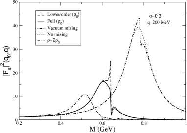
Figure 2: Pion form factor as a function of invariant mass ( $M=\sqrt{Q^{2}}$) with mean field including both vacuum and Fermi sea contributions. The dotted and dot dashed line represent pion form factor in vacuum without and with mixing respectively. The dashed and solid line depicts the same for $\alpha=0.3$, and $\rho=\rho_{0}$ in small angle approximation and for the arbitrary mixing angle respectively. The dot-dash-dashed line correspond to the case for arbitrary mixing angle at $\rho=2\rho_{0}$. “Full (lowest order)” corresponds to Eq.(20) (Eq.21)

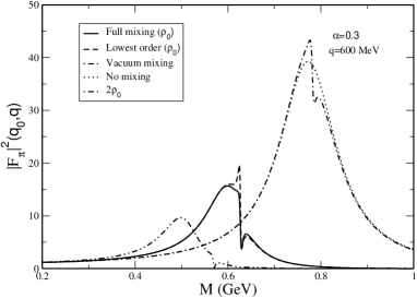
Figure 3: Same as Fig.2 with $q=600$ MeV.

In Fig. 4, we show the strong asymmetry dependence of the mixing which shifts the pole of the pion form factor towards lower invariant mass region. Moreover, we also find that the results are quite sensitive to the asymmetry parameter ($\alpha$).

As an application of the density and asymmetry parameter dependent pion form factor, we calculate the pion annihilation cross section in nuclear matter.

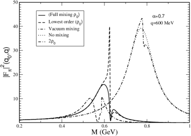
Figure 4: Same as Fig.3 for $\alpha=0.7$.

The dilepton production cross section is directly proportional to the square of the pion form factor and bears similar qualitative features. This is shown in Fig.5. For completeness, we also present results for the dilepton production rates for various combinations of density and asymmetry parameter at $T=100$ MeV in Fig. 6. Evidently the medium modified pion form factor leads to enhanced production of dileptons in the low invariant mass region.

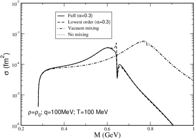
Figure 5: The cross section for $\pi^{+}\pi^{-}\rightarrow e^{+}e^{-}$.

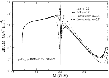
Figure 6: Dilepton production rate with and without mixing at two times the normal nuclear matter density.

5 Summary

In the present paper we have calculated pion form factor in asymmetric nuclear matter within the framework of relativistic mean field theory valid for arbitrarily large mixing angle. It is known that the vacuum pion form factor shows a shoulder like behaviour near the $\rho$ meson pole due to its admixture with the isoscalar $\omega$ meson indicating isospin symmetry violation. In this paper, we have discussed the possible enhancement of such mixing in asymmetric nuclear matter where unlike the vacuum case, this symmetry breaking is driven by the ground state due to the difference of neutron and proton densities. Automatically this would modify the pion form factor as we have shown. Another interesting aspect is the shift of pole position. This is related to the presence of scalar mean field leading to the reduced nucleon mass in matter. In-medium pion form factor naturally influences the pion annililation cross section which proceeds through an intermediate $\rho$ meson. Relativistic heavy ion collisions at GSI energies offers the unique opportunity to probe the in-medium pion form factor through dilepton measurements. Hence we have also calculated dilepton production rate due to pion annihilation in matter. In the low mass region the dilepton yield is enhanced due to dropping of vector meson mass as well as $\rho$-$\omega$ mixing.

We conclude with the comment that density and asymmetry dependent $\rho-\omega$ mixing is an interesting problem related to charge symmetry violation in matter and it could be worthwhile to extend the formalism developed in the present work to other approaches such as chiral perturbation theory and NJL model which have explicit chiral symmetry.

Appendix - I

Expressions for mixing angles and pion form factor

In this section we derive the expression for mixing angle and pion form factor for arbitrary mixing. In $\rho-\omega-\sigma$ model because of the possibility of scalar-vector mixing the mixed polarization tensor has the following form in ANM,

$$\Pi=\pmatrix{\Pi_{\rho\rho}&\Pi_{\rho\omega}&\Pi_{\rho\sigma}\cr\Pi_{\omega\rho}&\Pi_{\omega\omega}&\Pi_{\omega\sigma}\cr\Pi_{\sigma\rho}&\Pi_{\sigma\omega}&\Pi_{\sigma\sigma}}.$$ (24)

The propagator in the presence of mixining is the solution of

$$D^{-1}=D_{0}^{-1}-\Pi,$$ (25)

where $D_{0}={\mathrm{diag}}(d_{\rho},d_{\omega},d_{\sigma})$ with $d_{i}=1/(Q^{2}-m_{i}^{2}+i\epsilon),i=\rho,\omega,\sigma$.

The mixed propagator can be obtained by matrix inversion:

$$D=\left(\begin{array}[]{lll}\frac{s_{\sigma}s_{\omega}-\Pi_{\sigma\omega}\Pi_{\omega\sigma}}{\Delta}&\frac{\Pi_{\rho\sigma}\Pi_{\sigma\omega}-s_{\sigma}\Pi_{\rho\omega}}{\Delta}&\frac{\Pi_{\rho\omega}\Pi_{\omega\sigma}-s_{\omega}\Pi_{\rho\sigma}}{\Delta}\\ \frac{\Pi_{\sigma\rho}\Pi_{\omega\sigma}-s_{\sigma}\Pi_{\omega\rho}}{\Delta}&\frac{s_{\rho}s_{\sigma}-\Pi_{\rho\sigma}\Pi_{\sigma\rho}}{\Delta}&\frac{\Pi_{\rho\sigma}\Pi_{\omega\rho}-s_{\rho}\Pi_{\omega\sigma}}{\Delta}\\ \frac{\Pi_{\sigma\omega}\Pi_{\omega\rho}-s_{\omega}\Pi_{\sigma\rho}}{\Delta}&\frac{\Pi_{\rho\omega}\Pi_{\sigma\rho}-s_{\rho}\Pi_{\sigma\omega}}{\Delta}&\frac{s_{\rho}s_{\omega}-\Pi_{\rho\omega}\Pi_{\omega\rho}}{\Delta}\end{array}\right),$$ (26)

where $\Delta=s_{\rho}s_{\sigma}s_{\omega}-\Pi_{\rho\sigma}\Pi_{\sigma\rho}s_{\omega}-s_{\sigma}\Pi_{\rho\omega}\Pi_{\omega\rho}+\Pi_{\rho\sigma}\Pi_{\sigma\omega}\Pi_{\omega\rho}+\Pi_{\rho\omega}\Pi_{\sigma\rho}\Pi_{\omega\sigma}-s_{\rho}\Pi_{\sigma\omega}\Pi_{\omega\sigma}$.

The polarization functions in $D$ correspond to the mixing of the pure isospin eigenstates, $\rho_{I},\omega_{I}$ and $\sigma_{I}$. This matrix can be expressed in terms of the propagators of the physical $\rho,\omega$ and $\sigma$ fields which is an admixture of the pure states. This is achieved by appropriate field rotation involving various mixing angles in isospin space :

$$\pmatrix{\rho\cr\omega\cr\sigma}={\tilde{S}}\,\pmatrix{\rho_{I}\cr\omega_{I}\cr\sigma_{I}},$$ (27)

where $\tilde{S}$ is $3\times 3$ mixing matrix involving density dependent mixing angles. Let us first compare the polarization tensors $\Pi_{\omega\sigma}$ and $\Pi_{\rho\sigma}$ which have the same three momentum dependence. Now since $\Pi_{\omega\sigma}$ is a function of sum of the proton and neutron densities and $\Pi_{\rho\sigma}$ is that of the difference, thus $\Pi_{\omega\sigma}>>\Pi_{\rho\sigma}$ for small values of the asymmetry parameter $\alpha$. Taking $\Pi_{\rho\sigma}\approx 0$ the propagator matrix takes the form:

$$D=\left(\begin{array}[]{lll}\frac{s_{\sigma}s_{\omega}-\Pi_{\sigma\omega}\Pi_{\omega\sigma}}{\Delta_{1}}&-\frac{s_{\sigma}\Pi_{\rho\omega}}{\Delta_{1}}&\frac{\Pi_{\rho\omega}\Pi_{\omega\sigma}}{\Delta_{1}}\\ -\frac{s_{\sigma}\Pi_{\omega\rho}}{\Delta_{1}}&\frac{s_{\rho}s_{\sigma}}{\Delta}&-\frac{s_{\rho}\Pi_{\omega\sigma}}{\Delta_{1}}\\ \frac{\Pi_{\sigma\omega}\Pi_{\omega\rho}}{\Delta_{1}}&-\frac{s_{\rho}\Pi_{\sigma\omega}}{\Delta_{1}}&\frac{s_{\rho}s_{\omega}-\Pi_{\rho\omega}\Pi_{\omega\rho}}{\Delta_{1}}\end{array}\right),$$ (28)

where $\Delta_{1}=s_{\rho}s_{\sigma}s_{\omega}-s_{\sigma}\Pi_{\rho\omega}\Pi_{\omega\rho}-s_{\rho}\Pi_{\sigma\omega}\Pi_{\omega\sigma}$

Now it is also known that the scalar-vector mixing vanishes in the limit of vanishing 3-momentum and is very small for low momentum. However, $\Pi_{\rho\omega}$ remains non-zero even for $\vec{q}=0$. It is also to be noted that medium dependent mixing effects are dominant only in the low momentum region which allows us to put $\Pi_{\omega\sigma}\approx 0$ in this limit [14]. Under these assumptions, $D$ reduces to block diagonal form in which $\sigma$ decouples from $\rho$ and $\omega$ so that we have,

$$D=\pmatrix{\frac{s_{\omega}}{s_{\omega}s_{\rho}-\Pi_{\rho\omega}^{2}}&\frac{\Pi_{\rho\omega}}{s_{\rho}s_{\omega}-\Pi_{\rho\omega}^{2}}&0\cr\frac{\Pi_{\rho\omega}}{s_{\rho}s_{\omega}-\Pi_{\rho\omega}^{2}}&\frac{s_{\rho}}{s_{\rho}s_{\omega}-\Pi_{\rho\omega}^{2}}&0\cr 0&0&1/s_{\sigma}}.$$ (29)

Consequently, $\tilde{S}$ takes the form

$${\tilde{S}}=\pmatrix{\cos{\epsilon}&\sin{\epsilon}&0\cr-\sin{\epsilon}&\cos{\epsilon}&0\cr 0&0&1}.$$ (30)

We henceforth work in the $2\times 2$ subspace of $\rho$ and $\omega$, i. e. we use :

$$S=\pmatrix{\cos{\epsilon}&\sin{\epsilon}\cr-\sin{\epsilon}&\cos{\epsilon}}.$$ (31)

The mixing angle can be deduced by diagonalising the vector meson propagator [1]:

$$S^{-1}\pmatrix{\frac{s_{\omega}}{s_{\omega}s_{\rho}-\Pi_{\rho\omega}^{2}}&\frac{\Pi_{\rho\omega}}{s_{\rho}s_{\omega}-\Pi_{\rho\omega}^{2}}\cr\frac{\Pi_{\rho\omega}}{s_{\rho}s_{\omega}-\Pi_{\rho\omega}^{2}}&\frac{s_{\rho}}{s_{\rho}s_{\omega}-\Pi_{\rho\omega}^{2}}}S=\pmatrix{\frac{s_{\omega}}{s_{\rho}s_{\omega}-\Pi_{\rho\omega}^{2}}&0\cr 0&\frac{s_{\rho}}{s_{\rho}s_{\omega}-\Pi_{\rho\omega}^{2}}},$$ (32)

from which we obtain

$$\tan{2\epsilon}=\frac{2\Pi_{\rho\omega}}{s_{\rho}-s_{\omega}}.$$ (33)

In the small mixing angle limit the above equation reduces to

$$\epsilon=\frac{\Pi_{\rho\omega}}{s_{\rho}-s_{\omega}}.$$ (34)

For the derivation of pion form factor for arbitrary mixing angle we need to evaluate the matrix element for the process $\gamma\rightarrow\pi\pi$, which can be written as

$${\cal{M}}_{\gamma\rightarrow\pi\pi}^{\mu} = \pmatrix{{\cal{M}}_{\rho_{I}\rightarrow\pi\pi}^{\mu}&0}SS^{-1}\pmatrix{\frac{s_{\omega}}{s_{\rho}s_{\omega}-\Pi_{\rho\omega}^{2}}&\frac{\Pi_{\rho\omega}}{s_{\rho}s_{\omega}-\Pi_{\rho\omega}^{2}}\cr\frac{\Pi_{\rho\omega}}{s_{\rho}s_{\omega}-\Pi{\rho\omega}^{2}}&\frac{s_{\rho}}{s_{\rho}s_{\omega}-\Pi_{\rho\omega}^{2}}}$$ (35)

$$\times\,SS^{-1}\pmatrix{{\cal{M}}_{\gamma\rightarrow\rho_{I}}\cr{\cal{M}}_{\gamma\rightarrow\omega_{I}}}$$

where it is assumed that $\Gamma_{\omega_{I}\rightarrow\pi\pi}=0$. The physical amplitudes can be obtained from the above equation which are as follows :

$${\cal{M}}_{\rho\rightarrow\pi\pi}^{\mu} = \cos{\epsilon}{\cal{M}}_{\rho_{I}\rightarrow\pi\pi}^{\mu},$$

$${\cal{M}}_{\omega\rightarrow\pi\pi}^{\mu} = \sin{\epsilon}{\cal{M}}_{\rho_{I}\rightarrow\pi\pi}^{\mu},$$

$${\cal{M}}_{\gamma\rightarrow\rho} = \cos{\epsilon}{\cal{M}}_{\gamma\rightarrow\rho_{I}}-\sin{\epsilon}{\cal{M}}_{\gamma\rightarrow\omega},$$

$${\cal{M}}_{\gamma\rightarrow\omega} = \sin{\epsilon}{\cal{M}}_{\gamma\rightarrow\rho_{I}}+\cos{\epsilon}{\cal{M}}_{\gamma\rightarrow\omega}$$ (36)

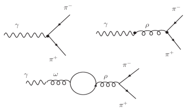
Figure 7: Contribution to $\rho$-$\omega$ mixing to pion form factor.

Thus the amplitude for $\gamma\rightarrow\pi\pi$ can be written as

$${\cal{M}}_{\gamma\rightarrow\pi\pi}^{\mu} = {\cal{M}}_{\rho\rightarrow\pi\pi}^{\mu}\frac{s_{\omega}}{s_{\rho}s_{\omega}-\Pi_{\rho\omega}^{2}}{\cal{M}}_{\gamma\rightarrow\rho}$$ (37)

$$+{\cal{M}}_{\rho\rightarrow\pi\pi}^{\mu}\frac{s_{\rho}}{s_{\rho}s_{\omega}-\Pi_{\rho\omega}^{2}}$$

$$\times{\tan\epsilon}{\cal{M}}_{\gamma\rightarrow\omega}$$

With these it is very easy to read out pion electromagnetic form factor from Fig.(7),

$$F_{\pi}(Q^{2}) = 1-g_{\rho\pi\pi}\frac{s_{\omega}}{s_{\rho}s_{\omega}-\Pi_{\rho\omega}^{2}}\frac{Q^{2}}{g_{\rho}}-g_{\rho\pi\pi}\tan{\epsilon}$$ (38)

$$\times\frac{s_{\rho}}{s_{\rho}s_{\omega}-\Pi_{\rho\omega}^{2}}\frac{Q^{2}}{g_{\omega}}$$

which in the small angle limit reduces to Eq.(20).

Appendix - II

In this appendix the mathematical expressions for polarization functions are presented.

$$\Pi_{\mu\nu}^{vv} = \frac{g_{i}g_{j}}{\pi^{3}}\left[A_{\mu\nu}-C_{\mu\nu}\right]$$

$$\Pi_{\mu\nu}^{vt+tv} = -\frac{g_{i}g_{j}}{\pi^{3}}\frac{(\kappa_{i}+\kappa_{j})M^{\ast}}{4M}B_{\mu\nu}$$

$$\Pi_{\mu\nu}^{tt} = -\frac{g_{i}g_{j}}{\pi^{3}}\frac{\kappa_{i}\kappa_{j}}{4M^{2}}\left[Q^{2}A_{\mu\nu}+M^{\ast\ 2}B_{\mu\nu}\right]$$ (39)

$$A_{\mu\nu} = Q^{2}\int\frac{d^{3}k}{E_{k}^{\ast}}\frac{{\cal{K}}_{\mu\nu}}{Q^{4}-4(K\cdot Q)^{2}}$$

$$= Q^{2}\,\int\,\frac{d^{3}k}{E_{k}^{\ast}}\,\frac{K_{\mu}K_{\nu}}{Q^{4}-4(K\cdot Q)^{2}}+\frac{Q_{\mu}Q_{\nu}}{4Q^{2}}({\tilde{B}}-\alpha(k_{f}))$$

$$-\frac{1}{4}\int\frac{d^{3}k}{E_{k}^{\ast}}(Q_{\mu}K_{\nu}+Q_{\nu}K_{\mu})\,\left[\frac{1}{Q^{2}-2K\cdot Q}\right.$$

$$-\left.\frac{1}{Q^{2}+2K\cdot Q}\right]$$

$$B_{\mu\nu} = Q^{4}\int\frac{d^{3}k}{E_{k}^{\ast}}\frac{Q_{\mu\nu}}{Q^{4}-4(K\cdot Q)^{2}}$$

$$C_{\mu\nu} = \int\frac{d^{3}k}{E_{k}^{\ast}}\frac{(K\cdot Q)^{2}Q_{\mu\nu}}{Q^{4}-4(K\cdot Q)^{2}}$$ (40)

$$A_{T} = Q^{2}\int\frac{d^{3}k}{E_{k}^{\ast}}\frac{k_{T}^{2}}{Q^{4}-4(K\cdot Q)^{2}}$$ (41)

$$= \frac{\pi}{4q}\int\frac{k^{3}dk}{E_{k}^{\ast}}{\cal{I}}_{2}$$

$$-\frac{\pi}{16q^{3}}\int\frac{kdk}{E_{k}^{\ast}}\left[\frac{}{}(Q^{4}+4E_{k}^{\ast\ 2}\omega^{2}){\cal{I}}_{2}-4Q^{2}E_{k}^{\ast}\omega{\cal{I}}_{1}\right.$$

$$-\left.8Q^{2}kq\right]$$

$$A_{L} = Q^{2}\int\frac{d^{3}k}{E_{k}^{\ast}}\frac{k_{z}^{2}-E_{k}^{\ast 2}}{Q^{4}-4(K\cdot Q)^{2}}-\frac{1}{4}({\tilde{B}}-\alpha(k_{f}))$$ (42)

$$+\frac{1}{2}\int\frac{d^{3}k}{E_{k}^{\ast}}(\omega E_{k}^{\ast}-q_{z}k_{z})$$

$$\times\left[\frac{1}{Q^{2}-2K\cdot Q}-\frac{1}{Q^{2}+2K\cdot Q}\right]$$

$$= \frac{\pi}{8q^{3}}\int\frac{kdk}{E_{k}^{\ast}}\left[(Q^{4}+4E_{k}^{\ast\ 2}\omega^{2}){\cal{I}}_{2}-4Q^{2}E_{k}^{\ast}\omega{\cal{I}}_{1}\right.$$

$$\left.-8Q^{2}kq\right]-\frac{\pi}{2q}\int kdkE_{K}^{\ast}{\cal{I}}_{2}$$

$$+\frac{\pi}{4q}\int\frac{kdk}{E_{k}^{\ast}}[Q^{2}{\cal{I}}_{2}-8kq]-\frac{1}{4}[{\tilde{B}}-\alpha(k_{f})]$$

$$B_{T} = B_{L}=B,C_{T}=C_{L}=C$$ (43)

$$B = Q^{4}\int\frac{d^{3}k}{E_{k}^{\ast}}\frac{1}{Q^{4}-4(K\cdot Q)^{2}}$$

$$= \frac{\pi Q^{2}}{2q}\int\frac{kdk}{E_{k}^{\ast}}{\cal{I}}_{2}$$

$$C = \int\frac{d^{3}k}{E_{k}^{\ast}}\frac{(K\cdot Q)^{2}}{Q^{4}-4(K\cdot Q)^{2}}$$

$$= \frac{\pi}{8q}\int\frac{kdk}{E_{k}^{\ast}}[Q^{2}{\cal{I}}_{2}-8kq]$$

$$\alpha(k_{f}) = \int_{0}^{k_{f}}\,\frac{d^{3}k}{E_{k}^{\ast}}$$

$$= 2\pi\left[k_{f}\epsilon_{f}-M^{\ast 2}\ln\frac{k_{f}+\epsilon_{f}}{M^{\ast}}\right]$$

$${\tilde{B}} = \frac{\pi Q^{2}}{2q}\int\frac{kdk}{E_{k}^{\ast}}{\cal{I}}_{1}$$ (44)

and

$${\cal{I}}_{1} = \ln\frac{Q^{4}-4(E_{k}^{\ast}\omega-kq)^{2}}{Q^{4}-4(E_{k}^{\ast}\omega+kq)^{2}}$$

$${\cal{I}}_{2} = \ln\frac{(Q^{2}+2kq)^{2}-4E_{k}^{\ast 2}\omega^{2}}{(Q^{2}-2kq)^{2}-4E_{k}^{\ast 2}\omega^{2}}$$ (45)

References

[1] H. B. O’connell, B. C. Pearce, A.W. Thomas and A.G. Williams,
Prog. Part. Nucl. Phys. 39, 201 (1997).
[2] J. Peikarewicz and A.G. Williams,
Phys. Rev. C 47, R2462(1993).
[3] G. A. Miller, A. K. Opper and E. J. Stephenson,
Ann. Rev. Nucl. Part. Sci. 56, 253 (2006).
[4] K. Okamoto, Phys. Lett 11, 150 (1964).
[5] J.A. Nolen, J.P. Schiffer,
Ann. Rev. Nucl. Part. Sc. 19, 471(1969).
[6] G.A. Miller , B.M.K. Nefkens and I. Slaus,
Phys. Rept. 194 1,(1990).
[7] A.K. Dutt-Mazumder, B. Dutta-Roy, A. Kundu,
Phys. Lett B 399, 196(1997).
[8] W. Broniowski and W. Florkowski,
Phys. Lett B 440,7(1998).
[9] S. Biswas and A. K. Dutt-Mazumder,
Phys. Rev. C 74, 065205 (2006).
nucl-th/0610058.
[10] A.K. Dutt-Mazumder, R. Hofmann, and M. Pospelov,
Phys. Rev. C 63, 015204 (2001).
[11] S. Zschocke and B. Kampfer,
Phys. Rev. C 70, 035207 (2004).
[12] B. Serot and J.D. Walecka, Adv. Nucl. Phys. 16(1986)1.
[13] P. Senger, J. Phys. G 28, 186 (2002).
[14] G. Wolf, B. Friman, and M. Soyeur, Nucl. Phys. A640
129 (1998).
[15] S. A, Chin, Ann. Phys. 108, 301(1977).
[16] T. Hatsuda, H. Shiomi and H. Kuwabara,
Prog. Theo. Phys. 95, 1009 (1996).
[17] S. Gardner and H. B. O’Connell, Phys. Rev. D 57
2716 (1998).
[18] W. Broniowski, W. Florkowski, and B. Hiller, Eur. Phys.
J. A7 287 (2000).
[19] W. Broniowski, W. Florkowski, Acta Phys. Polon B30
1079 (1999).
[20] W. Broniowski, W. Florkowski, and B. Hiller, Nucl. Phys.
A696 870 (2001).