Extraction and Interpretation of $\gamma N\rightarrow\Delta$ Form Factors
within a Dynamical Model
(From EBAC, Thomas Jefferson National Accelerator Facility)

Abstract

Within the dynamical model of Refs. [Phys. Rev. C54, 2660 (1996); C63, 055201 (2001)], we perform an analysis of recent data of pion electroproduction reactions at energies near the $\Delta(1232)$ resonance. We discuss possible interpretations of the extracted bare and dressed $\gamma N\rightarrow\Delta$ form factors in terms of relativistic constituent quark models and Lattice QCD calculations. Possible future developments are discussed.

I Introduction

One of the main challenges in hadron physics is to understand within Quantum Chromodynamics (QCD) the structure of the nucleon and its excited states. Through their couplings with the meson-baryon continuum, these excited states may be identified with the nucleon resonances ($N^{*}$) in various meson-baryon reactions. Ideally, one would like to study the $N^{*}$ structure by analyzing the meson-baryon reaction data completely within QCD. This however is far from our reach. As a compromise, one can analyze meson-baryon reaction data by developing reaction models within which both the internal structure of hadrons and the reaction mechanisms are modeled using theoretical guidances deduced from our current understanding of QCD. Of course, the separation between the reaction mechanisms and the internal structure of hadrons is by no means well defined theoretically. Thus the model dependence of the interpretations of the extracted $N^{*}$ parameters is unavoidable. This is not very satisfactory, but seems to be the only option we have at the present time. With this understanding, many models have been developed in recent years to analyze the very extensive electromagnetic meson production data which have been obtained by intense experimental efforts at Jefferson Laboratory (JLab), MIT-Bates, LEGS, Mainz, GRAAL, Bonn, and SPring-8. For a comprehensive review of the present experimental and theoretical status we refer the reader to Ref. burkertlee04 .

In this work we focus on recent measurements of pion electroproduction at energies near the $\Delta(1232)$ resonance, and in particular the data at $Q^{2}<$ 2.00 (GeV/c)² obtained at JLab joo02 ; smi06 , MIT-Bates bates and Mainz leu01 ; Sta06 ; Spa06 . One possible approach to analyze these data is to apply the dynamical model developed by Sato and Lee (SL) in Refs. satolee96 ; satolee01 . The SL model, as well as the unitary isobar model MAID maid , and the Dubna-Mainz-Taipei (DMT) model dmt have been used extensively to extract the $\gamma N\rightarrow\Delta$ form factors from the data. The SL model gives reasonably good descriptions of the very extensive data accumulated since 2001, using parameters obtained by analyzing the pion photoproduction data from LEGS legs and Mainz mainz , and the pion electroproduction data at $Q^{2}=2.8,4.0$ (GeV/c)² from JLab fro99 . In this paper, we would like to re-visit this model and to include the recent data joo02 ; smi06 ; bates ; leu01 ; Sta06 ; Spa06 in a comprehensive analysis to extract more precisely the $\gamma N\rightarrow\Delta$ form factors. Furthermore, we explore the theoretical interpretations of the extracted $\gamma N\rightarrow\Delta$ form factors in terms of two relativistic quark model calculations capstick-1 ; bruno-1 ; bruno-2 and a recent Lattice QCD calculation alexandrou .

In section II, we recall the essential ingredients of the SL model and present a refinement of the model from improvement of fits to the $\pi N$ scattering data. Section III is devoted to defining explicitly the $\gamma N\rightarrow\Delta$ transition form factors which are the focus of this work. The extraction of $\gamma N\rightarrow\Delta$ form factors from electroproduction data is discussed in section IV. We then discuss possible theoretical interpretations of the extracted $\gamma N\rightarrow\Delta$ form factors in section V. In section VI, we give a summary and discuss possible future developments.

II The SL model and $\pi N$ scattering

The essential feature of the SL model is to have a consistent description of both the $\pi N$ scattering and the electromagnetic pion production reactions. This is achieved by applying a unitary transformation method kso ; satolee96 to derive an effective Hamiltonian from the interaction Lagrangians with $N$, $\Delta$, $\pi$, $\rho$ ,$\omega$, and photon fields. The details of the model can be seen in Ref. satolee96 ; satolee01 . For our present purposes, it is sufficient to just recall the expression of the $\gamma N\rightarrow\pi N$ amplitude $T_{\pi N,\gamma N}$ given in Ref. satolee96

$$T_{\pi N,\gamma N}(E) = t_{\pi N,\gamma N}(E)+t^{R}_{\pi N,\gamma N}(E)\,,$$ (1)

where the non-resonant amplitude is defined by

$$t_{\pi N,\gamma N}(E)=[t_{\pi N,\pi N}(E)G_{\pi N}(E)+1]v_{\pi N,\gamma N}\,$$ (2)

with the non-resonant $\pi N$ scattering amplitude defined by

$$t_{\pi N,\pi N}(E)=v_{\pi N,\pi N}[1+G_{\pi N}(E)t_{\pi N,\pi N}(E)]\,.$$ (3)

Here $v_{\pi N,\pi N}$ is a $\pi N$ potential and $G_{\pi N}(E)$ is a $\pi N$ propagator with relativistic kinetic energy operators.

The resonant amplitude is given by

$$t^{R}_{\pi N,\gamma N}(E)=\frac{\bar{\Gamma}^{\dagger}_{\Delta,\pi N}\bar{\Gamma}_{\Delta,\gamma N}}{E-m_{\Delta}-\Sigma_{\Delta}(E)}\,,$$ (4)

where the dressed vertex interactions are defined, to the first order in electromagnetic coupling, by

$$\bar{\Gamma}^{\dagger}_{\Delta,\pi N} = [t_{\pi N,\pi N}(E)G_{\pi N}(E)+1]{\Gamma^{\dagger}}_{\Delta,\pi N}\,,$$ (5)

$$\bar{\Gamma}_{\Delta,\gamma N} = \Gamma_{\Delta,\gamma N}+{\Gamma}_{\Delta,\pi N}G_{\pi N}(E)t_{\pi N,\gamma N}\,.$$ (6)

In the above equations, $\Gamma_{\pi N,\Delta}$ and $\Gamma_{\Delta,\gamma N}$ are the bare vertex interactions. The energy shift $\Sigma_{\Delta}(E)$ is calculated from

$$\Sigma_{\Delta}(E)=\Gamma_{\Delta,\pi N}G_{\pi N}\bar{\Gamma}^{\dagger}_{\Delta,\pi N}\,.$$ (7)

Here we remark that the $\Delta$ propagator of Eq. (4) is the mathematical consequence of the Hamiltonian formulation of the reactions. It differs from the covariant forms, mainly used in tree-diagram models and extensively discussed in the literature on possible off-shell effects mukhopadhyay ; pascalutsa . The investigations on which covariant form of the $\Delta$ propagator is more consistent with the general principles of quantum field theory are continuing kirchbach .

By using Eqs.(2) and (3), one can write Eq.(6) as

$$\bar{\Gamma}_{\Delta,\gamma N}=\Gamma_{\Delta,\gamma N}+\delta\bar{\Gamma}_{\Delta,\gamma N}\,,$$ (8)

where

$$\delta\bar{\Gamma}_{\Delta,\gamma N}=\bar{\Gamma}_{\Delta,\pi N}G_{\pi N}(E)v_{\pi N,\gamma N}$$ (9)

with

$$\bar{\Gamma}_{\Delta,\pi N}=\Gamma_{\Delta,\pi N}[1+G_{\pi N}(E)t_{\pi N,\pi N}]\,.$$ (10)

We will discuss the dynamical content of the dressed vertices Eqs.(8)-(10) in section III.

Within the considered model the non-resonant $\pi N$ potential $v_{\pi N,\pi N}$ contains four mechanisms: the direct and crossed nucleon terms, $\rho$ exchange, and crossed $\Delta$ term. Apart from the standard $\pi NN$ coupling constant, the model is determined by three coupling constants $g_{\rho NN}g_{\rho\pi\pi}$ and $\kappa_{\rho}$ for the $\rho$-exchange, $f_{\pi N\Delta}$ for the $\pi N\rightarrow\Delta$ vertex. Each interaction vertex is regularized with a dipole form factor $F(k)=(\Lambda^{2}/(\Lambda^{2}+{\vec{k}}^{2}))^{2}$ where ${\vec{k}}$ is the pion momentum associated with the vertex. The model thus has additional three parameters: $\Lambda_{\pi NN}$ for the $\pi NN$ vertex, $\Lambda_{\pi N\Delta}$ for the $\pi N\Delta$ vertex and $\Lambda_{\rho}$ for both $\rho NN$ and $\rho\pi\pi$ vertices of the $\rho$-exchange term. These six parameters are adjusted along with the bare mass $m_{\Delta}$ of the $\Delta$ to fit the empirical $\pi N$ scattering phase shifts. We note that this model has considerably fewer parameters than the other $\pi N$ models used in the study of pion electroproduction calculations. For example, the $\pi N$ model hung used in the Dubna-Mainz-Taipei (DMT) model of pion electroproduction has 16 parameters. Thus we do not attempt to fit the data at energies above $T_{L}\sim 250$ MeV (invariant mass $W\sim 1280$ MeV). At higher energies, we expect that the coupling with the $\pi\pi N$ channel as well as the tails of higher mass $N^{*}$, such as the $P_{11}(1440)$ and $S_{11}(1535)$ resonances, must be included in a realistic description of the $\pi N$ scattering data. An extension of the SL model to higher energies has been developed recently in Ref. msl .

The original SL model (model L in Ref. satolee96 ) provides a quite good description of the $\pi N$ scattering phase-shifts up to $T_{L}\approx 250$ MeV except in the $P_{13}$ partial wave. This can be seen from comparing the data with the solid curves in Fig. 1. This discrepancy raised some questions concerning the stability of the results with respect to the $\pi N$ fit. In this work, we find that the fit to $P_{13}$ phase shifts can be considerably improved while retaining a similar quality of fit in the remaining partial waves. This is done by weighting the data in $P_{13}$ slightly more heavily in the fit. The resulting fits are the dotted curves in Fig. 1. The fitted parameters for the new $\pi N$ model (SL2) and the original SL model in Ref. satolee96 are compared in table 1. The remaining discrepancy in the $S_{31}$ channel at energies above $T_{L}\sim 150$ MeV perhaps can be resolved if we add additional mechanisms or use a different form factor parameterization. We have explored these possibilities and found that the model SL2 is the best we can have within the SL model.

It should be noted here that due to the lack of energy independent solutions at lower energies in the $P_{13}$ and $P_{31}$ partial waves, we have instead used the SAID said energy dependent solutions and assigned those points with $\approx 5\%$ errors in the fits. A more correct procedure is to fit the original $\pi N$ observables. This however is not pursued in this work.

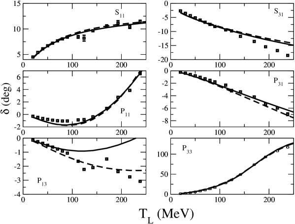
Figure 1: Phase shifts of $\pi N$ elastic scattering up to $T_{L}=$250 MeV. Solid and dotted stand for model SL and SL2 respectively. Data, $L_{2T,2J}$, are from the energy independent SAID said analysis plus 8 points from their energy dependent solution for the $P_{13}$ and $P_{31}$ partial waves at lower energies.

	Model
Parameter	SL2	SL  satolee96
$g_{\rho NN}g_{\rho\pi\pi}$	37.133	38.4329
$k_{\rho}$	2.8496	1.825
$\Lambda_{\pi NN}$	3.6177	3.2551
$\Lambda_{\rho}$	7.4639	6.2305
$\Lambda_{\pi N\Delta}$	3.2132	3.29
Bare $m_{\Delta}$	1296.9	1299.07
$[f_{\pi N\Delta}\sqrt{25/72}]$	1.1664	1.207
$g_{\omega NN}$	11.85	11.82
$G_{M}(0)$	1.86	1.85
$G_{E}(0)$	0.0251	0.025

Table 1: Parameters of the two considered models. The notations are explained in the text.

III The $\gamma^{*}N\rightarrow\Delta$ Form Factors

We now discuss the $\gamma N\rightarrow\Delta$ vertex interaction defined by Eq.(8). It has a bare vertex $\Gamma_{\Delta,\gamma N}$ and a term $\delta\bar{\Gamma}_{\Delta,\gamma N}$ which is determined by the non-resonant interaction $v_{\pi N,\gamma N}$ and a dressed $\pi N\rightarrow\Delta$ vertex $\bar{\Gamma}_{\Delta,\pi N}$. In the SL model, $v_{\pi N,\gamma N}$ contains the usual direct- and crossed-$N$ terms, $\pi$-exchange, contact term, crossed-$\Delta$ term, and $\rho$- and $\omega$-exchanges. Thus the dressed $\gamma N\rightarrow\Delta$ contains the meson loops illustrated in Fig. 2. We note that the mechanisms illustrated in Fig. 2 are similar to those in the calculations of the current matrix element $<\Delta|j^{\mu}_{em}\epsilon_{\mu}|N>$ within a hadron model where $N$ and $\Delta$ contain a pion cloud: $|B>=Z^{-1/2}[|B_{0}>+c_{1}|B_{0}\pi>+\dots]$. Such calculations can be found, for example, in Ref. liu using the cloudy bag model. Thus the term $\delta\bar{\Gamma}_{\Delta,\gamma N}$ is called the meson cloud contribution. Note that this definition is not shared by the DMT model.

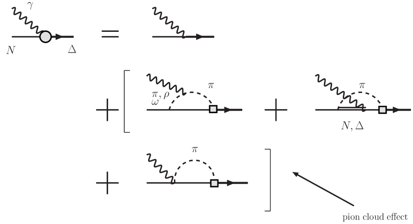
Figure 2: Graphic representation of the dressed $\gamma N\rightarrow\Delta$ vertex defined by Eq.(2.8)-(2.10).

In a consistent derivation using the unitary transformation method within the SL model, all strong interaction parameters except the $\omega NN$ vertex in $v_{\pi N,\gamma N}$ have been determined in fitting the $\pi N$ scattering data. The $\omega NN$ vertex coupling is determined by using the pion photoproduction data at $Q^{2}=0$, as will be further discussed later. By using the previous works on the $F_{\gamma NN}(Q^{2})$, $F_{\gamma\pi\pi}(Q^{2})$, and $F_{\gamma\pi V}(Q^{2})$ (with $V=\rho,\omega$) form factors, the non-resonant interaction $v_{\gamma N,\pi N}$ is then fixed at any $Q^{2}$, as explained in Ref. satolee01 . Since the dressed vertex $\bar{\Gamma}_{\Delta,\pi N}$ in Eq.(9) has also been fixed in fitting the $\pi N$ scattering data, the meson cloud term $\delta\bar{\Gamma}_{\Delta,\gamma N}$ can be predicted at any $Q^{2}$. With Eq.(8), the bare form factor $\Gamma_{\Delta,\gamma N}$ is then the only unknown, and can be extracted from the pion electroproduction data. This strategy of the SL model is also used in this work. Ideally, one should fit the $\pi N$ and electroproduction data simultaneously to minimize the errors in extraction. But this will be worthwhile only when the polarization data, such as those obtained by Kelly et al. kel05 , are also included in the fits. Our effort in this direction will be reported elsewhere.

One of the main objectives in this work is to explore the theoretical interpretations of the extracted bare $\gamma N\rightarrow\Delta$ vertex. We thus need to define this quantity precisely in the rest of this section. The bare vertex $\Gamma_{\Delta,\gamma N}$ of Eq.(6) is parameterized in the form developed by Jones and Scadron js73 . With the normalization $<{\vec{k}}|{\vec{k}^{\prime}}>=\delta({\vec{k}}-{\vec{k}^{\prime}})$ for the plane wave states and $<\phi_{B}|\phi_{B^{\prime}}>=\delta_{B,B^{\prime}}$ for $B=N$ and bare $\Delta$ states, we can write in the rest frame of the $\Delta$ and for the photon momentum $q=(\omega,{\bf q})$

$$<m_{j_{\Delta}},m_{t_{\Delta}}|\Gamma_{\Delta,\gamma N}(q)|\lambda_{\gamma}\lambda_{N},m_{t_{N}}> = F\langle{\textstyle{3\over 2}}m_{t_{\Delta}}|{\textstyle{1\over 2}}1m_{t_{N}}0\rangle$$ (11)

$$\times[M_{m_{j_{\Delta}},\lambda_{\gamma}\lambda_{N}}(q)G_{M}(Q^{2})+E_{m_{j_{\Delta}},\lambda_{\gamma}\lambda_{N}}(q)G_{E}(Q^{2})$$

$$+C_{m_{j_{\Delta}},\lambda_{\gamma}\lambda_{N}}(q)G_{C}(Q^{2})]$$

where $\lambda_{\gamma}$ and $\lambda_{N}$ are the helicities of the initial photon and nucleon, $m_{j_{\Delta}}$ is the z-component of the $\Delta$ spin, $m_{t_{\Delta}}$ and $m_{t_{N}}$ denote the isospin components, and

$$F=\frac{-e}{(2\pi)^{3/2}}\sqrt{\frac{E_{N}(\vec{q})+m_{N}}{2E_{N}(\vec{q})}}\frac{1}{\sqrt{2\omega}}\frac{3(m_{\Delta}+m_{N})}{4m_{N}(E_{N}(\vec{q})+m_{N})}$$ (12)

with

$$M_{m_{j_{\Delta}},\lambda_{\gamma}\lambda_{N}}(q) = <m_{j_{\Delta}}|i\vec{S}\times\vec{q}\cdot\vec{\epsilon}_{\lambda_{\gamma}}|\lambda_{N}>$$ (13)

$$E_{m_{j_{\Delta}},\lambda_{\gamma}\lambda_{N}}(q) = <m_{j_{\Delta}}|\vec{S}\cdot\vec{\epsilon}_{\lambda_{\gamma}}\vec{\sigma}\cdot\vec{q}+\vec{S}\cdot\vec{q}\vec{\sigma}\cdot\vec{\epsilon}_{\lambda_{\gamma}}|\lambda_{N}>$$ (14)

$$C_{m_{j_{\Delta}},\lambda_{\gamma}\lambda_{N}}(q) = \frac{1}{m_{\Delta}}<m_{j_{\Delta}}|\vec{S}\cdot\vec{q}\vec{\sigma}\cdot\vec{q}\epsilon_{0}|\lambda_{N}>$$ (15)

where $e=\sqrt{4\pi/137}$, photon polarization vector is defined by $\vec{\epsilon}_{\pm 1}=\frac{\mp}{\sqrt{2}}(\hat{x}\pm i\hat{y})$, and $\epsilon_{0}=0$ for $\lambda_{\gamma}=\pm 1$, $\epsilon_{0}=1$ and $\vec{\epsilon}_{0}=0$ for the scalar component $\lambda_{\gamma}=0$. The transition spin $\vec{S}$ is defined by $<j_{\Delta}m_{\Delta}|S_{m}|j_{N}m_{N}>=<j_{\Delta}m_{\Delta}|j_{N}1m_{N}m>$.

The form factors $G_{M}(Q^{2})$, $G_{E}(Q^{2})$, and $G_{C}(Q^{2})$ describe magnetic M1, Electric E2, and Coulomb C2 transitions. Choosing the photon direction $\vec{q}$ in the z-direction, the above matrix elements are related to the helicity amplitudes defined by Particle Data Group pdg (PDG)

$$A_{3/2}(Q^{2}) = B<m_{j_{\Delta}}=3/2,m_{t_{\Delta}}=m_{t_{N}}|\Gamma_{\Delta,\gamma N}(q)|\lambda_{\gamma}=+1\lambda_{N}=-1/2,m_{t_{N}}>$$ (16)

$$A_{1/2}(Q^{2}) = B<m_{j_{\Delta}}=1/2,m_{t_{\Delta}}=m_{t_{N}}|\Gamma_{\Delta,\gamma N}(q)|\lambda_{\gamma}=+1,\lambda_{N}=1/2,m_{t_{N}}>$$ (17)

$$S_{1/2}(Q^{2}) = B<m_{j_{\Delta}}=1/2,m_{t_{\Delta}}=m_{t_{N}}|\Gamma_{\Delta,\gamma N}(q)|\lambda_{\gamma}=0,\lambda_{N}=1/2,m_{t_{N}}>$$ (18)

with

$$B = \sqrt{\frac{(2\pi)^{3}E_{N}(\vec{q})\omega}{m_{N}K_{\gamma}}}$$ (19)

where

$$K_{\gamma}=\frac{m_{\Delta}^{2}-m_{N}^{2}}{2m_{\Delta}}$$ (20)

With $\vec{q}$ chosen in the z-direction, we can easily evaluate Eqs.(13)-(15). Eqs.(11) and (16)-(18) then lead to the following explicit relations

$$A_{3/2}(Q^{2}) = -\frac{\sqrt{3}A}{2}[G_{M}(Q^{2})+G_{E}(Q^{2})]\,,$$ (21)

$$A_{1/2}(Q^{2}) = -\frac{A}{2}[G_{M}(Q^{2})-3G_{E}(Q^{2})]\,,$$ (22)

$$S_{1/2}(Q^{2}) = -\frac{|\vec{q}|A}{\sqrt{2}m_{\Delta}}G_{C}(Q^{2})\,.$$ (23)

with

$$A = \frac{e}{2m_{N}}\sqrt{\frac{m_{\Delta}}{m_{N}K_{\gamma}}}\frac{|\vec{q}|}{1+Q^{2}/(m_{N}+m_{\Delta})^{2}}$$ (24)

The helicity amplitudes Eqs.(16)-(18) are most often calculated in hadron structure calculations. Eqs.(21)-(23) then allow comparisons of such calculations with the bare form factors $G_{M}(Q^{2})$, $G_{E}(Q^{2})$, $G_{C}(Q^{2})$ extracted from our analyses. These form factor are presumably sensitive to the short-range interquark interactions. They perhaps mainly contain information about the quark wavefunctions of the $N$ and $\Delta$ within the constituent quark model, as will be discussed in section V.

In Ref. satolee01 , it was found that the pion photoproduction data legs ; mainz and the electroproduction data at $Q^{2}=2.8,4.0$ GeV² fro99 can be fitted well by using the following naive parameterization

$$G_{x}(Q^{2})=G_{x}(0)\left(\frac{1}{1+Q^{2}/0.71({\rm GeV}/c)^{2}}\right)^{2}(1+a\,Q^{2})\,\exp(-b\,Q^{2})$$ (25)

where $x=M,E,C$, $a=0.154$ (GeV/c)² and $b=0.166$ (GeV/c)². The strengths at $Q^{2}=0$ are found to be $G_{M}(0)=1.85$, $G_{E}(0)=0.025$. The value of $G_{C}(0)$ was fixed using the long wavelength limit

$$G_{C}(0)=-4\frac{m^{2}_{\Delta}}{(m^{2}_{\Delta}-m^{2}_{N})}G_{E}(0)$$ (26)

Note that this ${\it ansatz}$ assumes an identical $Q^{2}$ dependence for all three ’bare’ electromagnetic couplings. There is no theoretical justification for this simple choice. Thus it is not clear whether the discrepancies between the predictions from the SL model (using the parameterization Eqs.(25)-(26) and the data accumulated since 2001 reflect information about the bare couplings or about deficiencies in the model description of the $\pi N$ rescattering process. With more data in a wide range of $Q^{2}$, we will abandon in this work the parameterization Eqs.(25-26) and directly extract these bare couplings by fitting the data at each individual $Q^{2}$ point.

The dressed form factor $\bar{\Gamma}_{\Delta,\gamma N}$ has the same symmetry property of the bare vertex defined above. Thus it can be expanded in the same form of Eq.(11). We denote the dressed quantities by $\bar{G}_{M}(Q^{2})$, $\bar{G}_{E}(Q^{2})$, $\bar{G}_{C}(Q^{2})$. The corresponding helicity amplitudes $\bar{A}_{\lambda}$ can also be calculated by using the same relations Eqs.(21)-(23). In Ref. satolee01 , it is shown that the dressed ratios can also be calculated from the imaginary parts of $M_{1+}$, $E_{1+}$ and $S_{1+}$ amplitudes of pion electroproduction

$$\bar{R}_{EM} = -\frac{\bar{G}_{E}}{\bar{G}_{M}}=\frac{{\rm Im}E_{1+}}{{\rm Im}M_{1+}}$$ (27)

$$\bar{R}_{SM} = \frac{|\vec{q}|}{2m_{\Delta}}\frac{\bar{G}_{C}}{\bar{G}_{M}}=\frac{{\rm Im}S_{1+}}{{\rm Im}M_{1+}}$$ (28)

It is common to define $G^{*}_{M}$ for the M1 transition form factor which is related to our dressed form factor by

$$G^{*}_{M}(Q^{2})=\sqrt{\frac{\Gamma^{exp}_{\Delta}}{\Gamma^{SL}_{\Delta}}}\frac{\bar{G}_{M}(Q^{2})}{\sqrt{1+Q^{2}/(m_{\Delta}+m_{N})^{2}}}$$ (29)

where $\Gamma^{exp}_{\Delta}=115$ MeV is used in extracting the data from $M^{3/2}_{1+}$ amplitude of pion electroproduction amplitude and $\Gamma^{SL}=93$ MeV from the SL model.

IV Extraction of $\gamma N\rightarrow\Delta$ Form Factors

With the refined $\pi N$ model SL2, we first re-analyze the $\pi^{0}$ photoproduction data. Here we need to also tune the less well determined parameters of the $\omega$-exchange $\gamma N\rightarrow\pi N$ non-resonant interaction. Following the procedure of Ref. satolee96 , we adjust the $\omega NN$ coupling constant $g_{\omega NN}$ and $G_{M}(0)$ and $G_{E}(0)$ of the bare $N$-$\Delta$ form factor to fit the data legs ; mainz of differential cross section and photon asymmetry $A_{\gamma}$ of the $\gamma N\rightarrow\pi N$ reaction. The $\omega NN$ form factor is assumed to be the same as that of $\rho NN$ which has been fixed in the fit to $\pi N$ data. The quality of the fit is comparable to what was achieved in Ref. satolee96 , and needs not be discussed here. The resulting values of $G_{M}(0)$ and $G_{E}(0)$ and $g_{\omega NN}$ are also listed in the last three lines of Table 1.

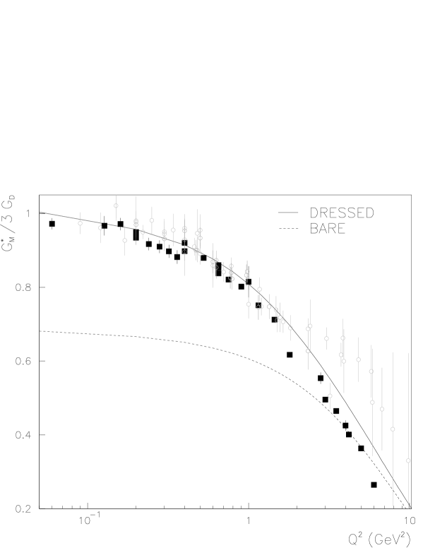
Figure 3: Magnetic dipole transition form factor $G^{*}_{M}$ for $\gamma^{*}N\rightarrow\Delta(1232)$, normalized to the proton dipole form factor $G_{D}(Q^{2})=1/[1+Q^{2}/\Lambda^{2}]^{2}$ with $\Lambda^{2}=0.71$ (GeV/c)². Experimental points are analyses of inclusive data ($\bigcirc$) from pre-1990 experiments at DESY and SLAC previousgm and recent exclusive $p(e,e^{\prime}p)\pi^{o}$ data ($\blacksquare$) from BATES bates , MAMI Sta06 ; Spa06 and JLAB joo02 ; smi06 ; kel05 ; fro99 ; ung06 . Solid curve is from the dressed calculation of this work using the parameterization of Eqs. (25)-(26). The dotted curve is obtained when the meson cloud effect, defined by Eq.(2.9) is turned off.

Figure 4: The ratios $\bar{R}_{EM}$ and $\bar{R}_{EM}$ (defined by Eqs.(3.17)-(3.18)) calculated from the dynamical model using the parameterization Eq.(3.15)-(3.16) (solid line). The data are from recent experiments at BATES: $\Box$ bates , MAMI: $\blacksquare$ leu01 , $\bigcirc$ Sta06 , $\bigtriangleup$ Spa06 , $\Diamond$ Pos01 , JLAB/CLAS: $\blacktriangledown$ smi06 , $\blacktriangle$ joo02 and JLAB/Hall A: $\bullet$ kel05 . CLAS points from Ref. smi06 were obtained from the average of UIM and SL model estimates in Table 2.

Our next step is to extract the $N$-$\Delta$ form factors by fitting all of the available pion electroproduction data at energies close to the $\Delta$ position. As a reference point for our analysis, we first use the parameterization Eqs.(25)-(26) of the SL model to make predictions. Our results, using that simple parameterization, for the dressed M1 form factors $G^{*}_{M}(Q^{2})$ and the ratios $\bar{R}_{EM}$ and $\bar{R}_{SM}$ are the solid curves shown in Figs. 3 and 4. The data shown here are from the analyses performed by the experimental groups using mainly the unitary isobar models maid ; azn03 . The data from our analyses, shown later in Fig.8, are not included in Figs. 3 and 4. The presence of two different extracted values for the same $Q^{2}$, in these and following figures, is due to the existence of two inconsistent data.

It is clear that the resulting dressed $G^{*}_{M}(Q^{2})$ (solid curve) agree well with the available empirical values. In the same figure, we also show the result (dashed curve) which is obtained by setting the meson cloud effects, $\delta\bar{\Gamma}_{\Delta,\gamma N}$ defined by Eq.(9), to zero. Clearly, the meson cloud effects are important in the low $Q^{2}$ region and gradually diminish as $Q^{2}$ increases. The predicted $R_{SM}$ (lower part of Fig. 4) also agree well with the data except at the two lowest $Q^{2}$ values $Q^{2}$ =0.06, 0.127 (GeV/c)² from the analyses by the MIT-Bates and Mainz groups.

Here we remark on the data presented in Figs. 3-4. Because the experiments so far do not have complete measurements including all polarization observables, the extraction of multipole amplitudes from the data needs some constraints imposed by making theoretical assumptions. The most common practice is to analyze the data starting from the amplitudes generated from the K-matrix isobar model MAID. We note that the data from the MIT-Bates and Mainz groups do not have the full coverage of angles and thus their extracted values of $\bar{R}_{EM}$ and $\bar{R}_{SM}$ perhaps depend very much on the dynamical content in MAID. The results from JLab at $Q^{2}>0.16$ (GeV/c)² are also analyzed using a unitarized isobar model (UIM) of Aznauryan azn03 . However the JLAB data cover almost the whole angular region and hence the fitted results are closer to a full partial wave analysis.

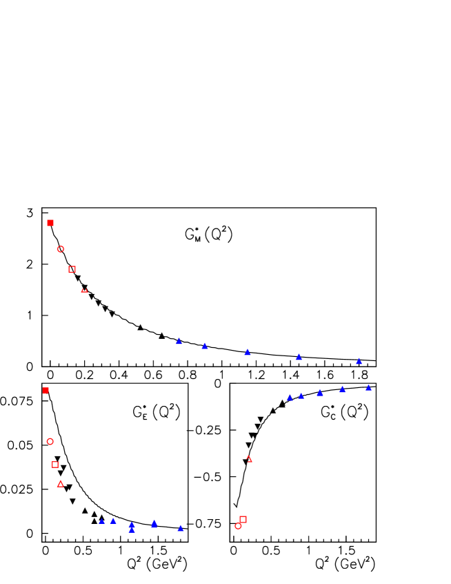
Figure 5: The dressed $\gamma N\rightarrow\Delta$ form factors (solid curves) calculated using the parameterization Eqs.(25)-(26) are compared with experiment. The data are from BATES: $\Box$ bates , MAMI: $\blacksquare$ leu01 , $\bigcirc$ Sta06 , $\bigtriangleup$ Spa06 and JLAB/CLAS: $\blacktriangledown$ smi06 , $\blacktriangle$ joo02 .

The ratios $\bar{R}_{EM}$ shown in the upper part of Fig. 4 clearly indicate that the parameterization Eq.(25) is not valid for $G_{E}(Q^{2})$. This can be seen more clearly in Fig. 5 where we compare each $N$-$\Delta$ form factor with the empirical values. To extract more precisely the $N$-$\Delta$ form factors, we therefore abandon the parameterization Eqs.(25)-(26) and perform $\chi^{2}$ fits to the available differential cross section data at each $Q^{2}$ by adjusting the values of the bare form factors. In Fig. 6, we show some results (solid curves) from our fits at $Q^{2}=0.06,0.127,0.2,0.9,1.45$ (GeV/c)². We see that the fits to the differential cross section data are better than predictions (dotted curves) using the parameterization Eqs.(25)-(26). The most visible fit improvement occurs in the longitudinal-transverse interference cross section $\sigma_{TL}$ at $Q^{2}=0.06,0.127$ (GeV/c)²

The resulting bare form factors are shown in Fig. 7. We now turn to discussing how these data on the bare $\gamma N\rightarrow\Delta$ can be interpreted theoretically.

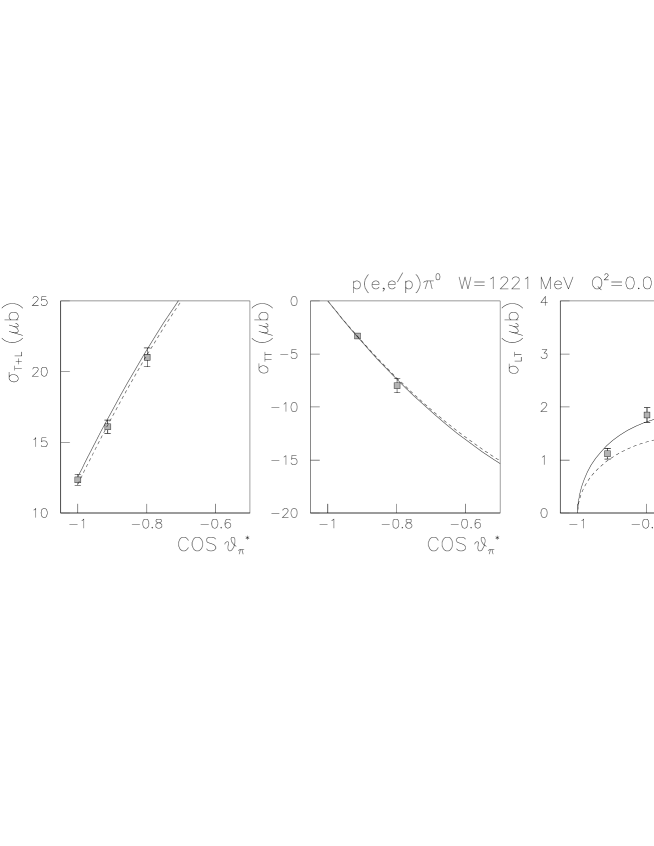
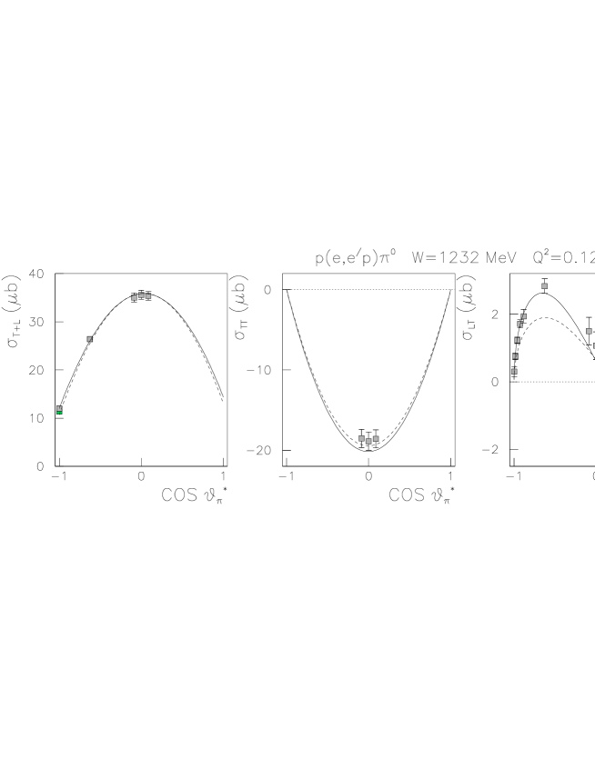
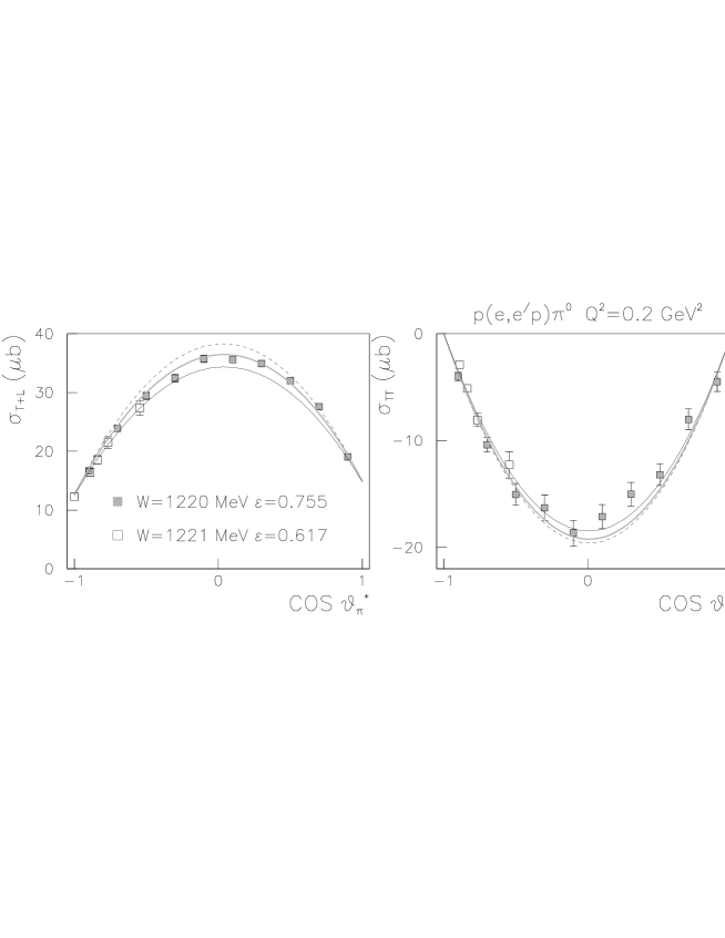
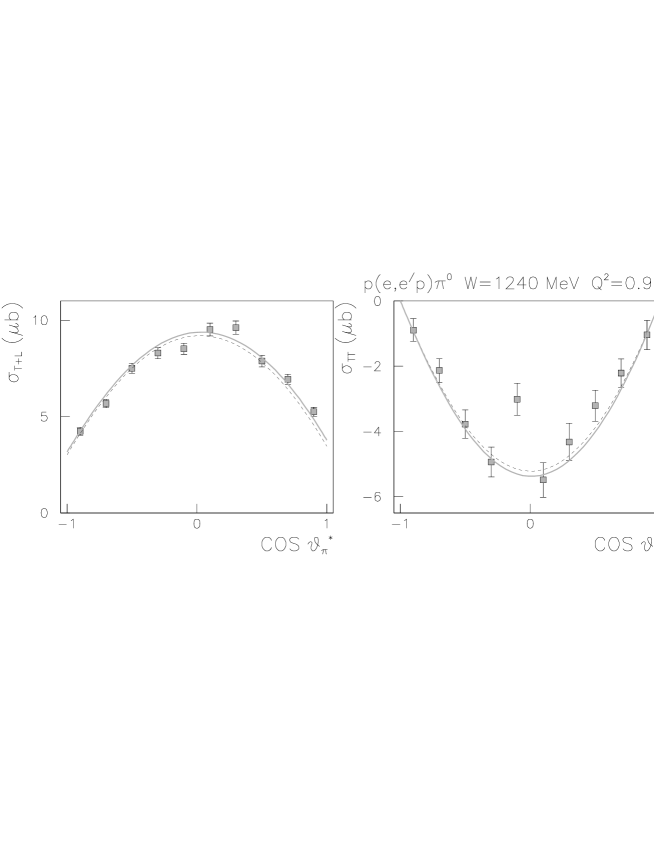
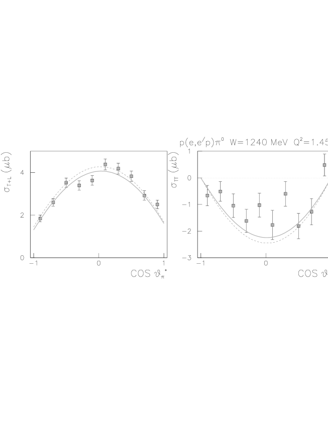
Figure 6: Fits to experimental $p(e,e^{\prime}p)\pi^{0}$ structure functions. Solid lines are from the fits with the bare form factors $G_{M}(Q^{2})$, $G_{E}(Q^{2})$ and $G_{C}(Q^{2})$ adjusted at each $Q^{2}$. The dashed curves are from the calculations using the parameterization Eqs.(3.15)-(3.16). Data are from MAMI Sta06 at $Q^{2}=0.06$ GeV², BATES bates at $Q^{2}=0.127$ GeV², CLAS smi06 ($W=1220$ MeV) and MAMI Spa06 ($W=1221$ MeV) at $Q^{2}=0.2$ GeV² and CLAS joo02 at $Q^{2}=0.9,1.45$ GeV².

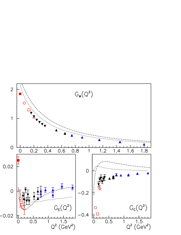
Figure 7: Bare form factors for the $\gamma N\to\Delta$ transition as a function of $Q^{2}$. The points have been obtained by performing individual fits for each $Q^{2}$ value to the corresponding pion electroproduction data (BATES: $\Box$ bates , MAMI: $\blacksquare$ leu01 , $\bigcirc$ Sta06 , $\bigtriangleup$ Spa06 and JLAB/CLAS: $\blacktriangledown$ smi06 , $\blacktriangle$ joo02 .) The dashed curves are from the front form quark model calculations of Refs. capstick-1 ; capstick-c . The dotted curves are from the instant form quark model calculations of Ref. bruno-1 .

V Theoretical Interpretations

To explore possible theoretical interpretations of the extracted $\Delta$ parameters, it is useful to first consider the electromagnetic pion production reaction within the general reaction theory feshbach . Like any reaction involving $composite$ systems, such as the atomic and nuclear reactions, its amplitude has a non-resonant part and a resonant part $T=t+t^{R}$ . Qualitatively speaking, the non-resonant amplitude $t$ is due to the fast process through some direct particle exchange mechanisms, and the resonant amplitude $t^{R}$ is due to the time-delayed process that the incoming particles lose their identities and an unstable system is formed and then decay into various final states. The unitarity condition ${\rm Im}T=T^{\dagger}T$ implies that $t$ and $t^{R}$ are not independent from each other. In the model considered in this work, this can be seen in Eqs.(4) for $t^{R}$ which contain the non-resonant amplitude $t$ through Eqs.(5)-(7). Thus the extracted dressed form factors $\bar{G}_{M}(Q^{2})$, $\bar{G}_{C}(Q^{2})$, $\bar{G}_{C}(Q^{2})$ of the resonant amplitude can only be compared with the hadron structure calculations of current matrix element $<\Delta|j^{\mu}_{em}\cdot\epsilon_{\mu}|N>$ which contain the meson loops illustrated in Fig. 2. Furthermore, these mesonic effects are dynamically identical to those in the non-resonant amplitude $t_{\pi N,\gamma N}=(1+t_{\pi N,\pi N})v_{\pi N,\gamma N}$ which is equally important in describing the data of reaction cross sections. We emphasize here that this close relation between the resonant and non-resonant amplitude is not specific to the formulation considered in this work, but is the consequence of a very general unitarity condition.

Clearly, it is a much more difficult task to understand the extracted dressed $\bar{G}_{M}(Q^{2})$, $\bar{G}_{E}(Q^{2})$, $\bar{G}_{C}(Q^{2})$ form factors within QCD. A simpler approach is to assume that the meson loops included in our model are the dominant mesonic effects resulting from the spontaneous breaking of chiral symmetry. It is then reasonable to compare our bare form factors ${G}_{M}(Q^{2})$, ${G}_{E}(Q^{2})$, ${G}_{C}(Q^{2})$ with hadron structure calculations in terms of only the constituent quark degrees of freedom. It is instructive to first consider the naive s-wave non-relativistic quark model within which the magnetic M1 transitions have a well known relation $\mu_{\Delta^{+}p}/\mu_{p}=2\sqrt{2}/3$ where

$$\frac{e}{2m_{p}}\mu_{p}=\langle p,m_{s_{N}}={\textstyle{1\over 2}}|\sum_{i}\frac{e_{i}}{2m_{q}}\sigma_{i}(z)|p,m_{s_{N}}={\textstyle{1\over 2}}\rangle$$ (30)

$$\frac{e}{2m_{p}}\mu_{\Delta^{+}p}=\langle\Delta^{+},m_{s_{\Delta}}={\textstyle{1\over 2}}|\sum_{i}\frac{e_{i}}{2m_{q}}\sigma_{i}(z)|p,m_{s_{N}}={\textstyle{1\over 2}}\rangle$$ (31)

Here $\mu_{p}$ is the proton magnetic moment with physical value $\mu^{exp}_{p}=1+\kappa_{p}\sim 2.77$, and $m_{q}$ is the constituent quark mass. From the above relation and the definition Eq.(11), one observe that the magnetic M1 form factor of $\gamma N\rightarrow\Delta$ at $Q^{2}=0$ can be directly calculated from the proton magnetic moment

$$G_{M}(0) = [\sqrt{2}G_{p}(0)]\left[\frac{2(E_{N}(q)+m_{N})}{3(m_{\Delta}+m_{N})}\right]\sqrt{\frac{2E_{N}(q)}{E_{N}(q)+m_{N}}}=0.84\mu_{p}$$ (32)

where $q=(m^{2}_{\Delta}-m^{2}_{N})/2m_{\Delta}\sim 260$ MeV/c. We thus observe that our bare value $G_{M}(0)=1.85$ can be understood in terms of constituent quark degrees of freedom only when we assume that the nucleon magnetic moment within the constituent quark model should be about $\sim 20\%$ less than the empirical value. The difference is from the meson loops, similar to that illustrated in Fig. 2. Such a mesonic correction is indeed close to what has been found in the cloudy bag model thomas , and is needed to explain the discrepancy between the data and the predictions from a covariant model based on the Dyson-Schwinger Equations roberts . On the other hand, our extracted bare E2 transition form factor $G_{E}(0)$ cannot be understood within the non-relativistic constituent quark model. With the tensor force within the conventional one-gluon-exchange, the estimated E2 transition of $\gamma N\rightarrow\Delta$ is known to be negligibly small compared with the value calculated from our value $G_{E}(0)=-0.025$.

We now discuss constituent quark model calculations of $\gamma N\rightarrow\Delta$ form factors. Since the $Q^{2}$ considered here is not very small, it is essential to perform calculations relativistically. We focus on two recent results from Capstick and Keister capstick-1 and Julia-Diaz and Riska bruno-1 . Both are within the framework of relativistic quantum mechanics outlined by Dirac dirac . There are three possible approaches within this framework: instant form, front form, and point form. The generators of instant form and front form can be defined within relativistic quantum field theory and hence are more closely related to the dynamical reaction model considered in this work. The calculation of Ref. capstick-1 is performed within the front form. The wavefunctions are expanded up to $N=6$ harmonic oscillator basis states in a variational calculation using a relativitized Hamiltonian capstick-2 which has a one-gluon exchange (OGE) short-distance interaction and Y-shaped string confinement. The tensor interactions and spin-orbit interactions are included in both the OGE and confining potentials. All of the potentials are smeared with some quark size, and momentum dependence of the potentials is parameterized in order to simulate off-shell effects. A quark form factor is included in this calculation capstick-c . We assume that this quark form factor is to account for the finite size of constituent quarks, not phenomenologically to include the meson loops as illustrated in Fig. 2. This conjecture is of course debatable and should be explored in future.

The calculation of Ref. bruno-1 starts with wavefunctions parameterized as $\phi_{0}(P)=N(1+\frac{P^{2}}{4b^{2}})^{-a}$ with $P=\sqrt{2(\vec{k}^{\,\,2}+\vec{q}^{\,\,2})}$, where $\vec{k}$ and $\vec{q}$ are two intrinsic momenta of the three-quark system, and $N$ is a normalization factor. The parameters $b$, $a$ and the constituent quark mass $m_{q}$ are adjusted to fit the nucleon electromagnetic form factors. With a phenomenological addition of d-state wavefunction, the same parameters are used to predict the $\gamma N\rightarrow\Delta$ form factors. Here we only consider their calculation within the instant form, mainly because it give the best fits to the data.

The comparisons of the predictions of Refs. capstick-2 and bruno-1 are given in Fig. 7. Clearly their results are only in qualitative agreements with the extracted bare form factors. In particular, both calculations fail to reproduce the very rapid drop of $G_{E}(Q^{2})$ from the photon point $Q^{2}=0$ to $Q^{2}=0.06$. Both calculations predict a sign change of $G_{C}(Q^{2})$ in disagreement with the extracted values.

In the fits (solid curves) shown in Fig. 6 for extracting the bare form factors, we of course also extract the dressed form factors. Their differences, which reflect the meson cloud effects defined by Eq.(9), can be seen by comparing the solid squares and triangles in Fig. 8. Obviously, pion cloud effects on $G_{E}(Q^{2})$ and $G_{C}(Q^{2})$ are very pronounced at low $Q^{2}$, as predicted in Ref. satolee01 . In the same figure, we also display the results from a recent Lattice QCD (LQCD) calculations alexandrou .

We now discuss the results from LQCD calculations. Currently LQCD can only be performed reliably with very large quark mass. There are two possible ways to use the extracted $\gamma N\rightarrow\Delta$ form factors to test these results. The first one is to conjecture that the meson-loop contributions in the quenched calculations is suppressed in the calculations with large quark mass and hence their results should be compared $directly$ with our bare values. The second one is to apply the chiral extrapolation to get results in the physical region with correct current quark masses. There are two problems in using the chiral extrapolation. First, it is only valid for low $Q^{2}$, although it has been used in a rather high $Q^{2}$ region. Second, there are higher order corrections on the commonly used chiral extrapolation, which have not been under control. The uncertainties due to this problem have been discussed by Pascalutsa and Vanderhaeghen pasc-3 . Thus it is not clear what to conclude from Fig. 8 for the results from LQCD of Ref. alexandrou . Further investigations are clearly needed.

Finally, we present our determined dressed $\bar{R}_{EM}$ and $\bar{R}_{SM}$ in the low $Q^{2}$ region where very large meson cloud effects have been identified in Fig. 8. Our results are listed in table 2 and compared with the values determined using the unitary isobar model (UIM). The difference between our values and that from the UIM reflect some model-dependence in the extraction.

	$\bar{R}_{EM}$(%)				$\bar{R}_{SM}$(%)
$Q^{2}$		UIM	SL	SL2		UIM	SL	SL2
0.16		-1.94(0.13)	-2.45(0.2)	-2.57(0.2)		-4.64(0.19)	-4.44(0.35)	-4.36(0.35)
0.20		-1.68(0.18)	-2.21(0.2)	-2.31(0.2)		-4.62(0.18)	-4.23(0.35)	-4.14(0.35)
0.24		-2.14(0.14)	-2.70(0.2)	-2.76(0.2)		-4.60(0.28)	-4.32(0.35)	-4.21(0.35)
0.28		-1.69(0.27)	-1.99(0.2)	-2.07(0.2)		-5.50(0.31)	-5.08(0.35)	-4.97(0.35)
0.32		-1.59(0.17)	-2.29(0.2)	-2.35(0.2)		-5.71(0.33)	-4.87(0.35)	-4.75(0.35)
0.36		-1.52(0.27)	-1.80(0.2)	-1.82(0.2)		-5.79(0.43)	-4.76(0.35)	-4.56(0.35)

Table 2: Extracted values of $E2/M1$ ratio $\bar{R}_{EM}$ and $C2/M1$ ratio $\bar{R}_{SM}=S_{1+}/M_{1+}$ at $Q^{2}=0.16-0.36$ GeV² from analysis of preliminary results from a CLAS measurement smi06 of the $p(e,e^{\prime}p)\pi^{0}$ reaction. Methods used are Unitary Isobar Model (UIM) and the SL and SL2 models described in this work. Errors are statistical only.

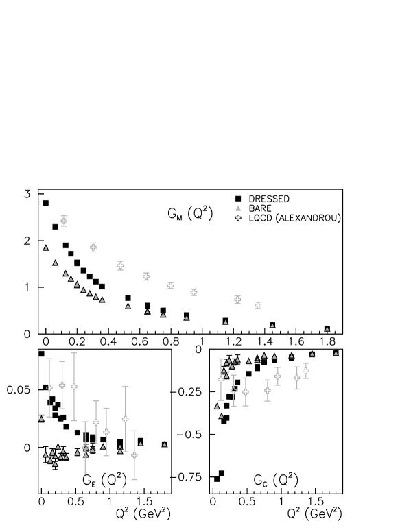
Figure 8: The extracted $\gamma N\rightarrow\Delta$ form factors. Dark squares(triangles) are the dressed (bare) values. Open squares are the lattice QCD calculation of Ref. alexandrou .

VI Discussion and summary

Within the dynamical model of Refs. satolee96 ; satolee01 we have performed a comprehensive analysis of recent pion electroproduction data to extract more precisely the $\gamma N\rightarrow\Delta$ form factors. It is found that the predictions from the original SL model are not changed much by improving its fit to the $\pi N$ phase shifts in $P_{13}$ channel. The fits to the very extensive $\pi^{0}$ electroproduction data near the $\Delta$ position can be improved when the simple parameterization Eqs.(25)-(26) is abandoned and the strengths of the bare form factors $G_{M}(Q^{2})$, $G_{E}(Q^{2})$, and $G_{C}(Q^{2})$ are adjusted at each $Q^{2}$ where the data are available.

In using our results, shown in Fig. 8 and table 2, to test hadron structure calculations, it is important to note that the differences between the dressed and bare $\gamma N\rightarrow\Delta$ form factors are from the meson loops illustrated in Fig. 2. We emphasize here that the parameters associated with these loops are the same as that in the non-resonant amplitude $t_{\pi N,\gamma N}$ and $t_{\pi N,\pi N}$ which are important components in describing both the $\pi N$ scattering phase shifts and pion electroproduction data. Thus the meson cloud effect identified in this analysis is well constrained by the reaction data directly. Such a direct connection with reaction data is very difficult to achieve in the current hadron model calculations, in particular the Lattice QCD.

As an exploratory step, we have considered two relativistic constituent quark model calculations of $\gamma N\rightarrow\Delta$ form factors. The predictions from both models differ significantly from the extracted dressed values, in particular in the low $Q^{2}$ region. As seen in Fig. 7, their results for $G_{M}(Q^{2})$ and $G_{E}(Q^{2})$ qualitatively reproduce our bare values both in shapes and magnitudes. This seems to suggest that the hadron calculations without meson degrees of freedom could make contact with the reaction data through the bare from factors extracted from a dynamical analysis such as the one given in this work. The origin of the differences in the Coulomb form factor $G_{C}(Q^{2})$ seen in Fig. 7 is not clear. It will be interesting to explore whether the parameters within both models can be refined to remove these discrepancies and also improve their results for the bare $G_{M}(Q^{2})$ and $G_{E}(Q^{2})$.

It is still difficult to interpret the extracted form factors in terms the current LQCD calculations. The discrepancies shown in Fig. 8 indicate the need of a better understanding of the chiral extrapolation used in obtaining those results as well as a significant improvement in LQCD calculations.

To end this paper, we mention that the non-resonant amplitude $t_{\pi N,\gamma N}$, which is crucial in evaluating the meson cloud effects on the $\gamma N\rightarrow\Delta$ form factors, can be more sensitively determined in the energy region away from the $\Delta$ position. While the SL model considered in this work can account for the data in the region of $W\sim 1100-1300$ MeV very well in most cases burkertlee04 , a more extensive analysis of the data away from the $\Delta$ position must be performed in the near future when polarization data will also become more extensive. Our effort in this direction to further improve our understanding of the $\gamma N\rightarrow\Delta$ form factors is in progress.

- (1) V. D. Burkert and T. S. H. Lee, Int. J. Mod. Phys. E 13, 1035 (2004).
- (2) K. Joo et al. (CLAS Collaboration), Phys. Rev. Lett. 88, 122001 (2002).
- (3) L.C. Smith et al. (CLAS Collaboration), to appear in Proceedings of the Workshop ”Shape of Hadron”, Athens, 2006. Eds. C.N. Papanicolas and A.M. Bernstein, AIP (2006).
- (4) C. Mertz et al., Phys. Rev. Lett. 86, 2963 (2001); C. Kunz et al., Phys. Lett. B 564, 21 (2003); N. F. Sparveris et al., Phys. Rev. Lett 94, 022003 (2005).
- (5) R. Leukel, Ph.D. thesis, University of Mainz, 2001.
- (6) S. Stave et al., nucl-ex/0604013.
- (7) N. Sparveris, (private communciation) to appear in Proceedings of the Workshop ”Shape of Hadron”, Athens, 2006. Eds. C.N. Papanicolas and A.M. Bernstein, AIP (2006).
- (8) T. Sato and T.-S.H. Lee, Phys. Rev. C54, 2660 (1996).
- (9) T. Sato and T.-S.H. Lee, Phys. Rev. C63, 055201 (2001).
- (10) D. Drechsel, O. Hanstein, S.S. Kamalov, and L. Tiator, Nucl. Phys. A645, 145 (1999).
- (11) S. S. Kamalov and S. N. Yang, Phys. Rev. Lett. 83, 4494 (1999).
- (12) G. Blanpied et al., Phys. Rev. Lett. 79, 4337 (1997); Phys. Rev. C64, 025203 (2001).
- (13) R. Beck et al., Phys. Rev. C 61, 035204 (2000).
- (14) V. V. Frolov et al., Phys. Rev. Lett. 82, 45 (1999).
- (15) S. Capstick and B.D. Keister, Phys. Rev. 51, 3598 (1995).
- (16) B. Julia-Diaz and D. O. Riska, Nucl. Phys. A 757, 441 (2005).
- (17) B. Julia-Diaz, D. O. Riska, and F. Coester, Phys. Rev. C 69 035212 (2004).
- (18) C. Alexandrou et al., Phys. Rev. D69, 114506 (2004); C. Alexandrou, P. de Forcrand, H. Neff, J. W. Negele, W. Schroers and A. Tsapalis, Phys. Rev. Lett. 94, 021601 (2005); C. Alexandrou, T. Leontiou, J. W. Negele and A. Tsapalis, hep-lat/0608051.
- (19) M. Kobayashi, T. Sato, and H. Ohtsubo, Prog. Theor. Phys. 98, 927 (1997).
- (20) M. Benmerrouche, R. M. Davidson and N. C. Mukhopadhyay, Phys. Rev. C 39, 2339 (1989).
- (21) V. Pascalutsa, Phys. Rev. D 58, 096002 (1998), and earlier references therein.
- (22) M. Napsuciale, M. Kirchbach, S. Rodriguez, Eur. Phys. J. A29, 289 (2006), and earlier references therein.
- (23) C.-T. Hung, S.N. Yang, and T.-S. H. Lee, Phys. Rev. C64, 034309 (2001).
- (24) A. Matsuyama, T. Sato, and T.-S. H. Lee, e-print Archive nucl-th/068051.
- (25) R. A. Arndt, W. J. Briscoe, I. I. Strakovsky and R. L. Workman, Phys. Rev. C 74, 045205 (2006); http://gwdac.phy.gwu.edu.
- (26) D.H. Lu, A.W. Thomas, A.G. Williams, Phys. Rev. C55, 3108 (1997).
- (27) J.J. Kelly, Phys. Rev. C 72, 048201 (2005); J.J. Kelly et al., Phys. Rev. Lett. 95, 102001 (2005).
- (28) H.F. Jones and M.D. Scadron, Ann. of Phys. 81, 1 (1973).
- (29) Particle Data Group, D.E. Groom et al., Eur. Phys. J. 15, 1 (2000).
- (30) W. Bartel et al., Phys. Lett. 28 B, 148 (1968); J. C. Adler et al., Nucl. Phys. B 46, 573 (1972); S. Stern et al., Phys. Rev. D 12, 1884 (1975); L.M. Stuart et al., Phys. Rev. D 58, 032003 (1998).
- (31) M. Ungaro et al. (CLAS Collaboration), Phys. Rev. Lett. 97, 112003 (2006).
- (32) Th. Pospischil et al., Phys. Rev. Lett. 86, 2959 (2001).
- (33) I. G. Aznauryan, Phys. Rev. C 67, 015209 (2003).
- (34) H. Feshbach Theoretical Nuclear Physics: Nuclear Reactions (Wiley, New York, 1992).
- (35) A.W. Thomas, Adv. Nucl. Phys., 13, 1-137 (1984).
- (36) R. Alkofer. A. Höll, M. Kloker, A. Krassnigg, C.D. Roberts, Few Body Syst. 37, 1 (2005); A. Höll et al., Nucl. Phys. A755, 298 (2005).
- (37) P.A.M. Dirac, Rev. Mod. Phys. 49, 392 (1949).
- (38) S. Capstick and N. Isgur, Phys.Rev. D34, 2809 (1986).
- (39) S. Capstick, private communication.
- (40) V. Pascalutsa and M. Vanderhaeghen, Phys. Rev. D 73, 034003 (2006).