Nuclear matter with Brown-Rho-scaled
Fermi liquid interactions

Abstract

We present a description of symmetric nuclear matter within the framework of Landau Fermi liquid theory. The low momentum nucleon-nucleon interaction $V_{{\rm low}-k}$ is used to calculate the effective interaction between quasiparticles on the Fermi surface, from which we extract the quasiparticle effective mass, the nuclear compression modulus, the symmetry energy, and the anomalous orbital gyromagnetic ratio. The exchange of density, spin, and isospin collective excitations is included through the Babu-Brown induced interaction, and it is found that in the absence of three-body forces the self-consistent solution to the Babu-Brown equations is in poor agreement with the empirical values for the nuclear observables. This is improved by lowering the nucleon and meson masses according to Brown-Rho scaling, essentially by including a scalar tadpole contribution to the meson and nucleon masses, as well as by scaling $g_{A}$. We suggest that modifying the masses of the exchanged mesons is equivalent to introducing a short-range three-body force, and the net result is that the Brown-Rho double decimation brown5 is accomplished all at once.

I Introduction

Landau’s theory of normal Fermi liquids landau1 ; landau2 ; landau3 describes strongly interacting many-body systems in terms of weakly interacting quasiparticles. Provided that the quasiparticles lie sufficiently close to the Fermi surface, they will be long-lived and constitute appropriate degrees of freedom for the system. The central aim of the theory is to determine the quasiparticle interaction, either phenomenologically or microscopically, with which it is possible to describe the low-energy, long-wavelength excitations of the system. This, in turn, is sufficient for the description of many bulk equilibrium properties of the interacting Fermi system. The initial application of Fermi liquid theory to nuclear physics was the phenomenological description of finite nuclei and nuclear matter by Migdal migdal1 ; migdal2 , and later a microscopic approach to Fermi liquid theory based on the Brueckner-Bethe-Goldstone reaction matrix theory was developed by Bäckman backman and others brown1 ; poggioli to describe nuclear matter. Although the latter approach was quantitatively successful, it was observed poggioli that Brueckner-Bethe-Goldstone theory is less reliable in the vicinity of the Fermi surface due to the use of angle-averaged Pauli operators and the unsymmetrical treatment of particle and hole self energies, which leads to an unphysical energy gap at the Fermi surface.

With the recent development of a nearly universal low-momentum nucleon-nucleon (NN) interaction $V_{{\rm low}-k}$ bogner1 derived from renormalization group methods, the application of Fermi liquid theory to nuclear matter has received renewed attention schwenk1 ; schwenk2 ; schwenk3 . The strong short-distance repulsion incorporated into all high-precision NN potential models is integrated out in low momentum interactions, rendering them suitable for perturbation theory calculations. Although limited Brueckner-Hartree-Fock studies kukei indicate that saturation is not achieved with $V_{{\rm low}-k}$ at a fixed momentum cutoff $\Lambda$, it has recently been shown bogner2 that by supplementing $V_{{\rm low}-k}$ with the leading-order chiral three-nucleon force, nuclear matter does saturate, thereby justifying the use of $V_{{\rm low}-k}$ in studies of nuclear matter.

Although many properties of the interacting ground state are beyond the scope of Fermi liquid theory, the quasiparticle interaction is directly related to several nuclear observables, including the compression modulus, symmetry energy, and anomalous orbital gyromagnetic ratio. As originally shown by Landau, the quasiparticle interaction is obtained from a certain limit of the four-point vertex function in the particle-hole channel. It is well known that using realistic NN interactions in the lowest order approximation to the quasiparticle interaction is insufficient to stabilize nuclear matter, as evidenced by a negative value of the compression modulus. This general phenomenon is observed in our calculations with $V_{{\rm low}-k}$ as well. However, stability is achieved by treating the exchange of density, spin, and isospin collective excitations to all orders in perturbation theory. The inclusion of these virtual collective modes in the quasiparticle interaction is carried out through the induced interaction formalism of Babu and Brown babu , which was originally developed for the description of liquid ³He and later applied to nuclear matter by Sjöberg sjoberg1 ; sjoberg2 . Subsequent work dickhoff ; backman2 has confirmed the importance of the induced interaction in building up correlations around a single quasiparticle, thereby increasing the compression modulus.

Our study is motivated in part by the work of Schwenk et al. schwenk1 , who were able to predict the spin-dependent parameters of the quasiparticle interaction from the experimentally extracted spin-independent parameters. Crucial to these calculations was a novel set of sum rules, derived from the induced interaction formalism, based on a similar treatment by Bedell and Ainsworth bedell to liquid ³He. In this paper we present a fully self-consistent solution to the Babu-Brown induced interaction equations for symmetric nuclear matter. Our iterative solution turns out to be qualitatively similar to the results of schwenk1 , but we find that at nuclear matter density the compression modulus and symmetry energy are smaller than the experimentally observed values while the anomalous orbital gyromagnetic ratio is too large, suggesting the possibility that important phenomena have been neglected.

We propose to extend this study by including hadronic modifications associated with the partial restoration of chiral symmetry at nuclear matter density, as suggested in brownrho . In this scenario, referred to as Brown-Rho scaling, the dynamically generated hadronic masses drop in the approach to chiral restoration, and at nuclear matter density it is expected that the masses of the light hadrons (other than the masses of the pseudoscalar mesons, which are protected by their Goldstone nature) decrease by approximately 20%. The success of one-boson-exchange and chiral EFT potentials in describing the nucleon-nucleon interaction suggests that a modification of meson masses in medium ought to have verifiable consequences in low energy nuclear physics. Although there is much current theoretical and experimental effort devoted to the program of assessing these medium modifications, the consequences for low-energy nuclear physics have yet to be fully explored.

Applying the mass scaling suggested in brownrho to our calculations of nuclear matter, we obtain a set of Fermi liquid coefficients in better agreement with both experiment and the nontrivial sum rules derived in schwenk1 . Explicit three-body forces, though essential for a complete description of nuclear matter, have been neglected in this study. However, we argue that modifying the vector meson masses is equivalent to including a specific short-ranged three-body force. We conclude with a discussion of the consequences of Brown-Rho scaling on the tensor force, which is diminished by the increasing strength of $\omega$-meson exchange.

II Fermi liquid theory

In this section we present a short description of Fermi liquid theory and its application to nuclear physics with emphasis on the microscopic foundation of the theory. The main assumption underlying Landau’s description of many-body Fermi systems is that there is a one-to-one correspondence between states of the ideal system and states of the interacting system. As one gradually turns on the interaction, the noninteracting particles become “dressed” through interactions with the many-body medium and evolve into weakly interacting quasiparticles. The interacting system is in many ways similar to an ideal system in that the classification of energy states remains unchanged and there is a well-defined Fermi surface, but the quasiparticles acquire an effective mass $m^{*}$ and finite lifetimes $\tau\sim(k-k_{F})^{-2}$. The energy of the interacting system is a complicated functional of the quasiparticle distribution function, and in general the exact dependence is inaccessible. But one can extract important information about bulk properties of the system by considering small changes in the distribution function. Expanding to second order, one finds

$$\delta E=\sum_{{\bf k}_{1}}\epsilon_{{\bf k}_{1}}^{(0)}\delta n({\bf k}_{1})+\frac{1}{2\Omega}\sum_{{\bf k}_{1},{\bf k}_{2}}f({\bf k}_{1},{\bf k}_{2})\delta n({\bf k}_{1})\delta n({\bf k}_{2})+{\cal O}(\delta n^{3}).$$ (1)

In this equation $\Omega$ is the volume of the system, $\epsilon_{{\bf k}_{1}}^{(0)}$ is the energy added to the system by introducing a single quasiparticle with momentum ${\bf k}_{1}$ (note that for $|{\bf k}_{1}|\equiv k_{1}=k_{F}$, $\epsilon_{{\bf k}_{1}}^{(0)}$ is just the chemical potential), and $f({\bf k}_{1},{\bf k}_{2})$ describes the interaction between two quasiparticles.

Since the quasiparticle interaction $f({\bf k}_{1},{\bf k}_{2})$ is the fundamental quantity of interest in Fermi liquid theory, we will carefully discuss its properties and its relationship to nuclear observables. Assuming the interaction to be purely exchange, it can be written as

$$f({\bf k}_{1},{\bf k}_{2})=\frac{1}{N_{0}}[F({\bf k}_{1},{\bf k}_{2})+F^{\prime}({\bf k}_{1},{\bf k}_{2})\tau_{1}\cdot\tau_{2}+G({\bf k}_{1},{\bf k}_{2})\sigma_{1}\cdot\sigma_{2}+G^{\prime}({\bf k}_{1},{\bf k}_{2})\tau_{1}\cdot\tau_{2}\sigma_{1}\cdot\sigma_{2}],$$ (2)

where we have factored out the density of states per unit volume at the Fermi surface, $N_{0}=\frac{2m^{*}k_{F}}{\hbar^{2}\pi^{2}}$, which leaves dimensionless Fermi liquid parameters denoted by $F,G,F^{\prime},G^{\prime}$. The spin-orbit interaction is neglected because it vanishes in the long wavelength limit in which we will be interested. Also, we have not included tensor operators (which would greatly complicate our calculation) because the tensor force contributes almost completely in second order, as shown in the original paper by Kuo and Brown kb , as an effective central interaction in the ${}^{3}S_{1}$ state. In schwenk1 the tensor Fermi liquid parameters for symmetric nuclear matter were calculated from $V_{{\rm low}-k}$ in which the dominant second-order contributions from one-pion exchange were included. Since quasiparticles are well-defined only near the Fermi surface, we assume that $k_{1}=k_{F}=k_{2}$. In this case the dimensionless Fermi liquid parameters $F,F^{\prime},G,G^{\prime}$ depend on only the angle between ${\bf k}_{1}$ and ${\bf k}_{2}$, which we call $\theta$. Then it is convenient to perform a Legendre polynomial expansion as follows

$$F({\bf k},{\bf k}^{\prime})=\sum_{l}F_{l}P_{l}(\mbox{cos }\theta),\hskip 7.22743ptG({\bf k},{\bf k}^{\prime})=\sum_{l}G_{l}P_{l}(\mbox{cos }\theta),\mbox{ etc.}$$ (3)

The Fermi liquid parameters $F_{l},G_{l},\dots$ decrease rapidly for larger $l$, and so there are only a small number of parameters that can either be fit to experiment or calculated microscopically.

In the original application of the theory to liquid ³He and nuclear systems, the quasiparticle interaction was obtained phenomenologically by fitting the dimensionless Fermi liquid parameters to relevant data. For nuclear matter several important relationships exist between nuclear observables and the Fermi liquid parameters. Galilean invariance can be used landau1 to connect the Landau parameter $F_{1}$ to the quasiparticle effective mass

$$\frac{m^{*}}{m}=1+F_{1}/3.$$ (4)

Adding a small number of neutrons and removing the same number of protons from the system will increase and decrease, respectively, the density of protons and neutrons in the system (and therefore the Fermi energies of the two species). The change in the energy, described by the symmetry energy $\beta$, can be related migdal2 to the Landau parameter $F_{0}^{\prime}$

$$\beta=\frac{\hbar^{2}k_{F}^{2}}{6m^{*}}(1+F_{0}^{\prime}).$$ (5)

In a similar way, the equal increase or decrease of the proton and neutron densities leads to a relationship between the scalar-isoscalar Landau parameter $F_{0}$ and the compression modulus ${\cal K}$

$${\cal K}=\frac{3\hbar^{2}k_{F}^{2}}{m^{*}}\left(1+F_{0}\right).$$ (6)

Finally, it can be shown migdal2 that an odd nucleon added just above the Fermi sea induces a polarization of the medium leading to an anomalous contribution to the orbital gyromagnetic ratio of the form

$$g_{l}^{p} = [1-\delta g_{l}]\mu_{N}$$

$$g_{l}^{n} = [\delta g_{l}]\mu_{N},$$ (7)

where $\delta g_{l}$ is given by

$$\delta g_{l}=\frac{1}{6}\frac{F^{\prime}_{1}-F_{1}}{1+F_{1}/3}.$$ (8)

Clearly there are certain values of the Landau parameters that are physically unreasonable. For instance, if $F_{1}<-3$ or $F_{0}<-1$, the effective mass or compression modulus would be negative. Quite generally it can be shown pomeranchuk that the Landau parameters must satisfy stability conditions

$$X_{l}>-(2l+1),$$ (9)

where $X$ represents $F,G,F^{\prime},G^{\prime}$.

A rigorous foundation for the assumptions underlying Landau’s theory can be obtained through formal many-body techniques abrikosov ; nozieres . It is not our goal to reproduce the original arguments landau3 , but rather to give a clear motivation for the diagrammatic expansion leading to the quasiparticle interaction. Starting from the usual definition of the four-point Green’s function in momentum space

$$G_{\alpha\beta,\gamma\delta}(k_{1},k_{2};k_{3},k_{4})=(2\pi)^{8}\delta^{(4)}(k_{1}+k_{2}-k_{3}-k_{4})[G_{\alpha\gamma}(k_{1})G_{\beta\delta}(k_{2})\delta^{(4)}(k_{1}-k_{3})$$ (10)

$$-G_{\alpha\delta}(k_{1})G_{\beta\gamma}(k_{2})\delta^{(4)}(k_{2}-k_{3})+\frac{i}{(2\pi)^{4}}G(k_{1})G(k_{2})G(k_{3})G(k_{4})\Gamma_{\alpha\beta,\gamma\delta}(k_{1},k_{2};k_{3},k_{4})],$$

where $G(k_{1})$ is the Fourier transform of $G(xt,x^{\prime}t^{\prime})$ and $k_{1},\dots,k_{4}$ represent four-vectors (e.g. $k_{1}=({\bf k}_{1},\omega_{1}))$, it can be shown that the quasiparticle interaction is related to a certain limit of the four-point vertex function $\Gamma_{\alpha\beta,\gamma\delta}(k_{1},k_{2};k_{3},k_{4})$. From energy-momentum conservation ($k_{1}+k_{2}=k_{3}+k_{4}$) we can write $k_{3}-k_{1}=K=k_{2}-k_{4}$ and therefore define $\Gamma(k_{1},k_{2};K)=\Gamma(k_{1},k_{2};k_{3},k_{4})$. The important point is that since we are considering only low-energy long-wavelength excitations, the particle-hole energy-momentum $K$ should be small. We can write a Bethe-Salpeter equation for the fully reducible vertex function $\Gamma$ in terms of the ph irreducible vertex function $\tilde{\Gamma}$ in the direct channel with momentum transfer $K$:

$$\Gamma_{\alpha\beta,\gamma\delta}(k_{1},k_{2};K) = \tilde{\Gamma}_{\alpha\beta,\gamma\delta}(k_{1},k_{2};K)$$ (11)

$$-i\sum_{\epsilon,\eta}\int\frac{d^{4}q}{(2\pi)^{4}}\tilde{\Gamma}_{\alpha\epsilon,\gamma\eta}(k_{1},q;K)G(q)G(q+K)\Gamma_{\eta\beta,\epsilon\delta}(q,k_{2};K)$$

shown diagrammatically in Fig. 1.

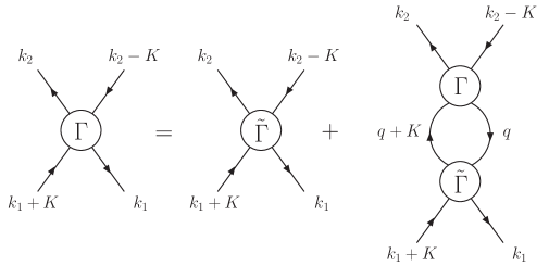
Figure 1: The Bethe-Salpeter equation for the fully irreducible vertex function $\Gamma$ in terms of the $ph$ irreducible vertex function $\tilde{\Gamma}$.

The product of propagators may have singularities in the limit that $K\rightarrow 0$, in which case the poles can be replaced by $\delta$-functions inside the integral:

$$G(q)G(q+K)=\frac{2i\pi z^{2}\hat{\bf q}\cdot{\bf K}}{\omega-v_{F}\hat{\bf q}\cdot{\bf K}}\delta(\epsilon-\mu)\delta(q-k_{F})+\phi({\bf q}),$$ (12)

where $z$ is the renormalization at the quasiparticle pole and $\phi({\bf q})$ accounts for the multipair background. The limit $K=(\omega,{\bf K})\to 0$ depends on the relative ordering of the two limits ${\bf K}\rightarrow 0$ and $\omega\rightarrow 0$. Defining

$$\Gamma^{\omega}(k_{1},k_{2}) = \lim_{\omega\rightarrow 0}\lim_{{\bf K}\rightarrow 0}\Gamma(k_{1},k_{2};K)\hskip 7.22743pt\mbox{ and}$$

$$\Gamma^{K}(k_{1},k_{2}) = \lim_{{\bf K}\rightarrow 0}\lim_{\omega\rightarrow 0}\Gamma(k_{1},k_{2};K),$$ (13)

from eq. (12) we see that the product of propagators is regular for $\Gamma^{\omega}$. Thus, to calculate $\Gamma^{\omega}$ we must first calculate the $ph$ irreducible diagrams belonging to $\tilde{\Gamma}$ and then iterate via the Bethe-Salpeter equation with the intermediate multipair background $\phi$. The $\delta$-function singularities in $\Gamma^{K}$ can be used to perform the integrals over $q_{0}$ and $|{\bf q}|$, and through algebraic manipulation it is possible to combine $\Gamma^{\omega}$ and $\Gamma^{K}$ into a single integral equation

$$\Gamma^{K}_{\alpha\beta,\gamma\delta}(k_{1},k_{2}) = \Gamma^{\omega}_{\alpha\beta,\gamma\delta}(k_{1},k_{2})$$ (14)

$$-\frac{1}{16\pi}N_{0}z^{2}\sum_{\epsilon,\eta}\int d\Omega_{q}\Gamma^{\omega}_{\alpha\epsilon,\gamma\eta}(k_{1},q)\Gamma^{K}_{\eta\beta,\epsilon\delta}(q,k_{2}).$$

Physically, $\Gamma^{\omega}$ represents the exchange of virtual excitations between quasiparticles, and $\Gamma^{K}$ represents the forward scattering of quasiparticles at the Fermi surface. By relating these vertex functions to the equations describing zero sound, Landau landau3 was able to make the identifications

$$f(k_{1},k_{2}) = z^{2}\Gamma^{\omega}(k_{1},k_{2})\hskip 7.22743pt\mbox{ and}$$

$$a(k_{1},k_{2}) = z^{2}\Gamma^{k}(k_{1},k_{2}),$$ (15)

where $f(k_{1},k_{2})$ is just the quasiparticle interaction introduced earlier and $a(k_{1},k_{2})$ is the physical scattering amplitude.

III Induced Interaction

In principle one could exactly calculate the quasiparticle interaction by summing up all $ph$ irreducible diagrams contributing to the $ph$ vertex function in the limit $k/\omega\rightarrow 0$. Since this is not practicable in general, one must limit the calculation to a certain subset of diagrams. We could proceed by calculating the relevant diagrams order by order, but this would miss an essential point, which we now elaborate. From eqs. (14) and (15), we see that the physical scattering amplitude $a(k_{1},k_{2})$ iterates the quasiparticle interaction to all orders through an integral equation shown schematically in Fig. 2.

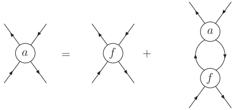
Figure 2: The diagrammatic relationship between the physical scattering amplitude $a$ and the quasiparticle interaction $f$.

If only a finite set of diagrams are included in the quasiparticle interaction, then the scattering amplitude will not be antisymmetric. For instance, if we include only the bare particle-hole antisymmetrized vertex shown in Fig. 3(a), then diagram (b) will be contained in the equation for the scattering amplitude but its exchange diagram, labeled (c), will not.

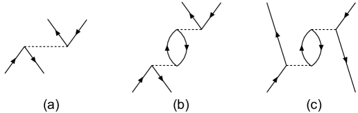
Figure 3: Diagrams contributing to the quasiparticle interaction $f$ and the scattering amplitude $a$. Diagrams (a) and (c) contribute to $f$, whereas all three contribute to $a$.

Quantitatively, the fact that the scattering amplitude is antisymmetric requires that it vanish in singlet-odd and triplet-odd states as the Landau angle $\theta$ approaches 0. This leads to two constraints landau3 ; friman on the Fermi liquid parameters in the form of sum rules:

$$\sum_{l}\left(\frac{F_{l}}{1+F_{l}/(2l+1)}+3\frac{G_{l}^{\prime}}{1+G_{l}^{\prime}/(2l+1)}\right)=0$$ (16)

$$\sum_{l}\left(\frac{2}{3}\frac{F_{l}}{1+F_{l}/(2l+1)}+\frac{F_{l}^{\prime}}{1+F_{l}^{\prime}/(2l+1)}+\frac{G_{l}}{1+G_{l}/(2l+1)}\right)=0$$ (17)

Clearly, the sum rules must be satisfied for the “correct” set of Fermi liquid parameters describing nuclear matter. To account for this infinite set of exchange diagrams, Babu and Brown babu proposed separating the quasiparticle interaction into a driving term and an induced term:

$$f(k,k^{\prime})=f_{d}(k,k^{\prime})+f_{i}(k,k^{\prime}),$$ (18)

where the induced interaction is defined to contain those diagrams that would be the exchange terms necessary to preserve the antisymmetry of $a(k_{1},k_{2})$. Then the induced interaction is given by a diagrammatic expansion shown in Fig. 4. Physically, the induced interaction represents that part of the quasiparticle interaction that results from the exchange of virtual collective modes, which can be classified as density, spin, or isospin excitations.

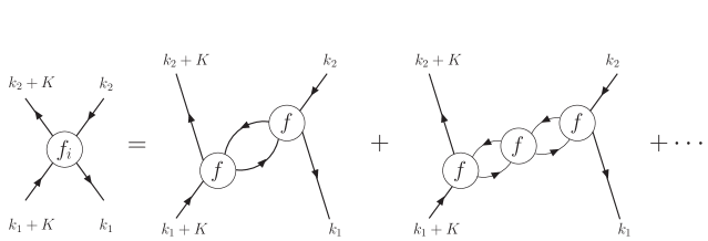
Figure 4: The diagrammatic form of the induced interaction. In the limit that $k_{1}=k_{2}$ it can be shown that the external lines exactly couple to particle-hole excitations through the $f$ function.

In the limit that ${\bf k}_{1}\rightarrow{\bf k}_{2}$ it can be rigorously proved babu that the coupling of quasiparticles to these collective excitations is precisely through the quasiparticle interaction itself, thereby justifying the diagrammatic expression in Fig. 4.

The relationship between the induced interaction and the full quasiparticle interaction was derived by Babu and Brown babu for liquid ³He and applied to nuclear matter by Sjöberg sjoberg1 . To lowest order in the Fermi liquid parameters, the induced interaction is given by

$$4F_{i} = \left[\frac{{F_{0}}^{2}}{1+F_{0}\alpha_{0}}+\frac{3{{F_{0}}^{\prime}}^{2}}{1+{F_{0}}^{\prime}\alpha_{0}}+\frac{{3G_{0}}^{2}}{1+G_{0}\alpha_{0}}+\frac{9{{G_{0}}^{\prime}}^{2}}{1+{G_{0}}^{\prime}\alpha_{0}}\right]\alpha_{0}$$

$$4G_{i} = \left[\frac{{F_{0}}^{2}}{1+F_{0}\alpha_{0}}+\frac{{3{F_{0}}^{\prime}}^{2}}{1+{F_{0}}^{\prime}\alpha_{0}}-\frac{{G_{0}}^{2}}{1+G_{0}\alpha_{0}}-\frac{3{{G_{0}}^{\prime}}^{2}}{1+{G_{0}}^{\prime}\alpha_{0}}\right]\alpha_{0}$$

$$4{F_{i}}^{\prime} = \left[\frac{{F_{0}}^{2}}{1+F_{0}\alpha_{0}}-\frac{{{F_{0}}^{\prime}}^{2}}{1+{F_{0}}^{\prime}\alpha_{0}}+\frac{{3G_{0}}^{2}}{1+G_{0}\alpha_{0}}-\frac{3{{G_{0}}^{\prime}}^{2}}{1+{G_{0}}^{\prime}\alpha_{0}}\right]\alpha_{0}$$

$$4{G_{i}}^{\prime} = \left[\frac{{F_{0}}^{2}}{1+F_{0}\alpha_{0}}-\frac{{{F_{0}}^{\prime}}^{2}}{1+{F_{0}}^{\prime}\alpha_{0}}-\frac{{G_{0}}^{2}}{1+G_{0}\alpha_{0}}+\frac{{{G_{0}}^{\prime}}^{2}}{1+{G_{0}}^{\prime}\alpha_{0}}\right]\alpha_{0}$$ (19)

where

$$\alpha_{0}=\alpha_{0}({\bf q},0)=\frac{1}{2}+\frac{1}{2}\left(\frac{q}{4k_{F}}-\frac{k_{F}}{q}\right){\rm ln}\frac{k_{F}-q/2}{k_{F}+q/2}$$ (20)

is the Lindhard function, which is related to the density-density correlation function $\chi_{\rho\rho}$ by

$$\chi_{\rho\rho}({\bf q},\omega)=\frac{-\alpha_{0}({\bf q},\omega)}{1+F_{0}\alpha_{0}({\bf q},\omega)},$$ (21)

and ${\bf q}={\bf k}_{1}-{\bf k}_{2}$. The interpretation of equation (19) is as follows. The Landau parameters in the numerator describe the coupling of quasiparticles to particular collective modes. For instance, the $F_{0}$ represents the coupling to density excitations, $G_{0}$ the coupling to spin excitations, etc., and the denominators enter from the summation of bubbles to all orders. Including the $l=1$ Fermi liquid parameters, the induced interaction is given by

$$4F_{i} = \left[\frac{{F_{0}}^{2}\alpha_{0}}{1+F_{0}\alpha_{0}}+\left(1-\frac{q^{2}}{4k_{F}^{2}}\right)\frac{{F_{1}}^{2}\alpha_{1}}{1+F_{1}\alpha_{1}}\right.+\frac{{3G_{0}}^{2}\alpha_{0}}{1+G_{0}\alpha_{0}}+\left(1-\frac{q^{2}}{4k_{F}^{2}}\right)\frac{{3G_{1}}^{2}\alpha_{1}}{1+G_{1}\alpha_{1}}$$ (22)

$$+ \frac{3{{F_{0}}^{\prime}}^{2}\alpha_{0}}{1+{F_{0}}^{\prime}\alpha_{0}}+\left(1-\frac{q^{2}}{4k_{F}^{2}}\right)\frac{3{{F_{1}}^{\prime}}^{2}\alpha_{1}}{1+{F_{1}}^{\prime}\alpha_{1}}+\left.\frac{9{{G_{0}}^{\prime}}^{2}\alpha_{0}}{1+{G_{0}}^{\prime}\alpha_{0}}+\left(1-\frac{q^{2}}{4k_{F}^{2}}\right)\frac{9{{G_{1}}^{\prime}}^{2}\alpha_{1}}{1+{G_{1}}^{\prime}\alpha_{1}}\right],$$

where $\alpha_{1}$ defined by

$$\alpha_{1}({\bf q},0)=\frac{1}{2}\left[\frac{3}{8}-\frac{k_{F}^{2}}{2q^{2}}+\left(\frac{k_{F}^{3}}{2q^{3}}+\frac{k_{F}}{4q}-\frac{3q}{32k_{F}}\right){\rm ln}\left(\frac{k_{F}+q/2}{k_{F}-q/2}\right)\right]$$ (23)

is related to the current-current correlation function, and analogous expressions hold for the spin- and isospin-dependent parts of the induced interaction. These equations were first obtained in backman2 , carried far enough to include velocity-dependent effects in terms of an effective mass, in the approximation of quadratic spectrum.

Having characterized the induced part of the quasiparticle interaction, let us now elaborate on the driving term. By definition, this component of the interaction consists of those diagrams that cannot be separated into two diagrams by cutting one particle line and one hole line. Some of the low order terms contributing to the driving term are shown in Fig. 5, where the interaction vertices are assumed to be antisymmetrized.

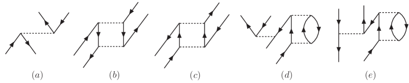
Figure 5: A selection of diagrams contributing to the driving term in the quasiparticle interaction. Diagrams (d) and (e) are included implicitly through the renormalization at the quasiparticle pole.

Some higher-order terms, such as diagram $(d)$ in Fig. 5, are included implicitly through the quasiparticle renormalization $z$ and need not be calculated explicitly, as described in detail in brown2 . In order to preserve the Pauli principle sum rules (16) and (17) the driving term must be antisymmetrized. Thus, including Fig. 5(d) requires that (e) also be included in order for the scattering amplitude to be antisymmetric.

IV Calculations and Results

According to the discussion in the previous section, the starting point of a microscopic derivation of the quasiparticle interaction is a calculation of the antisymmetrized driving term to some specified order in the bare potential. Nearly all previous calculations have used the $G$-matrix, since it is well known that the unrenormalized high-precision NN potentials are unsuitable for perturbation theory calculations due to the presence of a strong short-distance repulsion. The resummation of particle-particle ladder diagrams in the $G$-matrix softens the potential but introduces several undesirable features from the perspective of Fermi liquid theory. Most important is the unphysical gap in the single particle energy spectrum at the Fermi surface due to the fact that hole lines receive self-energy corrections but particle lines do not. In the past it was suggested poggioli ; sjoberg2 that introducing a model space, within which particles and holes are treated symmetrically, could overcome this difficulty.

An alternative method for taming the repulsive core is to integrate out the high momentum components of the interaction in such a way that the low energy dynamics are preserved bogner1 ; bogner3 . This is accomplished by rewriting the half-on-shell $T$-matrix

$$T(p^{\prime},p,p^{2})=V_{NN}(p^{\prime},p)+\frac{2}{\pi}{\cal P}\int_{0}^{\infty}\frac{V_{NN}(p^{\prime},q)T(q,p,p^{2})}{p^{2}-q^{2}}q^{2}dq$$ (24)

with an explicit momentum cutoff $\Lambda$, which yields the low momentum $T$-matrix defined by

$$T_{{\rm low}-k}(p^{\prime},p,p^{2})=V_{{\rm low}-k}(p^{\prime},p)+\frac{2}{\pi}{\cal P}\int_{0}^{\Lambda}\frac{V_{{\rm low}-k}(p^{\prime},q)T_{{\rm low}-k}(q,p,p^{2})}{p^{2}-q^{2}}q^{2}dq.$$ (25)

Enforcing the requirement that $T_{{\rm low}-k}(p^{\prime},p,p^{2})=T(p^{\prime},p,p^{2})$ for $p^{\prime},p<\Lambda$ preserves the low energy physics encoded in the scattering phase shifts. Remarkably, under this construction all high-precision NN potentials flow to a nearly universal low momentum interaction $V_{{\rm low}-k}$ as the momentum cutoff $\Lambda$ is lowered to $2.1$ fm^-1. In fact, $k=2.1$ fm^-1 is precisely the CM momentum beyond which the experimental phase shift analysis has not been incorporated in the high-precision NN interactions.

For an initial approximation to the driving term, we include the first-order antisymmetrized matrix element shown diagrammatically in Fig. 5(a) as well as the higher order diagrams, such as (d) and (e), that are included implicitly through the renormalization strength at the quasiparticle pole. The quasiparticles are confined to a thin model space $P$ near the Fermi surface

$$P=\lim_{\delta\to 0}\sum_{k_{F}<k<k_{F}+\delta}|\vec{k}\rangle\langle\vec{k}|,$$ (26)

and the first-order contribution is given by

$$\langle\vec{k}_{1}\vec{k}_{2}ST|V|(\vec{k}_{3}\vec{k}_{4}-\vec{k}_{4}\vec{k}_{3})ST\rangle=\langle k,\theta ST|V|k,\theta ST\rangle,$$ (27)

where $k_{1}=k_{2}=k_{3}=k_{4}=k_{F}$, $\theta$ is the angle between the two momenta, and the relative momentum $k=k_{F}\mbox{sin}(\theta/2)$. Given the $V_{{\rm low}-k}$ matrix elements in the basis $|klSTJ\rangle$, we project onto the central components and change from a spherical wave basis to a plane wave basis. Then the dimensionful driving term is given by

$$\langle kST|V_{d}|kST\rangle=z^{2}\frac{4\pi}{2S+1}\sum_{J,l}(2J+1)(1-(-1)^{l+S+T})\langle klSJT|V_{{\rm low-}k}|klSJT\rangle.$$ (28)

Inserting the form of the quasiparticle interaction in eq. (2) into the left hand side of eq. (28), we obtain the Fermi liquid parameters in terms of $V_{ST}(k)=\langle kST|V|kST\rangle$. The result is

$$f = \;\;\,\frac{1}{16}V_{00}+\frac{3}{16}V_{01}+\frac{3}{16}V_{10}+\frac{9}{16}V_{11}$$

$$g = -\frac{1}{16}V_{00}-\frac{3}{16}V_{01}+\frac{1}{16}V_{10}+\frac{3}{16}V_{11}$$

$$f^{\prime} = -\frac{1}{16}V_{00}+\frac{1}{16}V_{01}-\frac{3}{16}V_{10}+\frac{3}{16}V_{11}$$

$$g^{\prime} = \;\;\,\frac{1}{16}V_{00}-\frac{1}{16}V_{01}-\frac{1}{16}V_{10}+\frac{1}{16}V_{11},$$ (29)

where the momentum dependence has been suppressed for simplicity. From eq. (4) it can be shown that

$$\frac{m^{*}}{m}=\frac{1}{1-\mu f_{1}/3},$$ (30)

where $\mu=2mk_{F}/\pi^{2}\hbar^{2}=\frac{m}{m^{*}}N_{0}$, from which we construct the dimensionless Fermi liquid parameters. In all of our calculations we include partial waves up to $J=6$. In Table 1 we show the Landau parameters of the driving term derived from three different low momentum interactions obtained from the Nijmegen I & II potentials wiringa and the CD-Bonn potential machleidt for a momentum cutoff of $\Lambda=2.1$ fm^-1 and a Fermi momentum of $k_{F}=1.36$ fm^-1. From the available theoretical analyses of nucleon momentum distributions pand , we take the quasiparticle renormalization strength to be $z=0.7$ for nuclear matter.

	Nijmegen I				Nijmegen II				CD-Bonn
$l$	$F_{l}$	$G_{l}$	$F^{\prime}_{l}$	$G^{\prime}_{l}$	$F_{l}$	$G_{l}$	$F^{\prime}_{l}$	$G^{\prime}_{l}$	$F_{l}$	$G_{l}$	$F^{\prime}_{l}$	$G^{\prime}_{l}$
0	-1.230	0.130	0.392	0.619	-1.475	0.248	0.549	0.583	-1.199	0.135	0.350	0.603
1	-0.506	0.241	0.252	0.118	-0.445	0.161	0.172	0.225	-0.498	0.240	0.259	0.118
2	-0.201	0.120	0.101	0.021	-0.213	0.127	0.106	0.020	-0.200	0.122	0.101	0.022
3	-0.110	0.054	0.051	0.009	-0.120	0.060	0.056	0.007	-0.111	0.055	0.051	0.010

Table 1: The Fermi liquid parameters of the NN interaction $V_{{\rm low}-k}$ derived from the Nijmegen potentials and CD-Bonn potential for a cutoff of $\Lambda=2.1$ fm^-1 and Fermi momentum 1.36 fm^-1.

The induced interaction is obtained by iterating equations (18) and (22) until a self-consistent solution is reached. The density-density and current-current correlation functions in (22) introduce a momentum dependence in the induced interaction, and the Fermi liquid parameters for the induced interaction are obtained by projecting onto the Legendre polynomials

$$F_{i,l}=\frac{2l+1}{2}\int_{-1}^{1}F_{i}(\theta)P_{l}(\mbox{cos }\theta)\,d(\mbox{cos }\theta),\mbox{ etc.}$$ (31)

For the first iteration we use the Landau parameters obtained from the bare low momentum interaction as an estimate for the full quasiparticle interaction in eq. (22). However, since $F_{0}$ does not satisfy the stability criteria (9) for either the Nijmegen or CD-Bonn potentials, in the first iteration we replace it in both cases with an arbitrary value that does. The convergence of the iteration scheme is generally rapid and relatively insensitive to the set of initial parameters chosen for the low-momentum Nijmegen I and CD-Bonn potentials. In contrast, the low momentum Nijmegen II potential exhibits poor convergence properties, though a solution to the coupled equations can still be found. For a completely consistent solution at each iteration we recalculate the driving term with the new effective mass.

The final self-consistent result for the quasiparticle interaction is shown in Fig. 6 for the CD-Bonn potential, and the Fermi liquid parameters for the driving term, induced interaction, and full quasiparticle interaction are shown in Table 2.

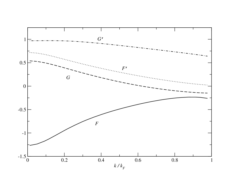
Figure 6: The self-consistent solution for the full quasiparticle interaction as a function of $k=\frac{1}{2}|{\bf k}_{1}-{\bf k}_{2}|$ derived from the low momentum CD-Bonn potential.

	Full				Driving				Induced
$l$	$F$	$G$	$F^{\prime}$	$G^{\prime}$	$F_{d}$	$G_{d}$	$F^{\prime}_{d}$	$G^{\prime}_{d}$	$F_{i}$	$G_{i}$	$F^{\prime}_{i}$	$G^{\prime}_{i}$
0	-0.476	0.025	0.221	0.784	-1.276	0.144	0.373	0.642	0.801	-0.119	-0.152	0.142
1	-0.335	0.263	0.273	0.171	-0.530	0.256	0.275	0.125	0.195	0.007	-0.002	0.048
2	-0.238	0.139	0.117	0.020	-0.212	0.130	0.107	0.024	-0.026	0.009	0.010	-0.003
3	-0.101	0.055	0.050	0.014	-0.119	0.059	0.054	0.011	0.018	-0.004	-0.004	0.003

Table 2: The self-consistent solution of the Babu-Brown equations for the low momentum CD-Bonn potential. The full Fermi liquid parameters are obtained by projecting the quasiparticle interaction in Fig. 6 onto the Legendre polynomials.

For comparison we list the Fermi liquid parameters obtained in schwenk1 where the spin-independent Landau parameters were taken from experiment and used to calculate the spin-dependent parameters with a set of nontrivial sum rules:

$F_{0}=-0.27$	$G_{0}=0.15\pm 0.3$	${F_{0}}^{\prime}=0.71$	${G_{0}}^{\prime}=1.0\pm 0.2$
$F_{1}=-0.85$	$G_{1}=0.45\pm 0.3$	${F_{1}}^{\prime}=0.14$	${G_{1}}^{\prime}=0.0\pm 0.2$

Although the experimental values for the spin-independent parameters are appreciably different from the self-consistent solution we have obtained, our values for the spin-dependent parameters fall within the errors predicted from the sum rules. However, the main effect of the induced interaction is to cut down the strong attraction in the spin-independent, isospin-independent part of the quasiparticle interaction. In fact, the repulsion in this channel coming from the induced interaction is large enough for the resulting $F_{0}$ to satisfy the stability condition in (9). The effective mass, compression modulus, and symmetry energy are shown in Table 3 together with the deviations $\delta S_{1}$ and $\delta S_{2}$ from the sum rules (16) and (17). We list the results for the three different bare potentials with a momentum cutoff of $\Lambda=2.1$ fm^-1. In calculating the contributions to (16) and (17) we have included Landau parameters for $l\leq 3$.

	Nijmegen I	Nijmegen II	CD-Bonn
$m^{*}/m$	0.887	0.930	0.888
${\cal K}$ [MeV]	136	102	136
$\beta$ [MeV]	18.1	20.5	17.6
$\delta g_{l}$ [$\mu_{N}$]	0.682	0.452	0.685
$\delta S_{1}$	0.20	0.16	0.27
$\delta S_{2}$	-0.04	-0.02	-0.04

Table 3: Nuclear observables obtained from the self-consistent solution of the Babu-Brown equations and deviations $\delta S_{1}$ and $\delta S_{2}$ from the Pauli principle sum rules.

The compression modulus for nuclear matter is extrapolated from the data on giant monopole resonances in heavy nuclei, with the expected value being $200-300$ MeV young ; steiner . The symmetry energy is determined by fitting the data on nuclear masses to various versions of the semi-empirical mass formula masses , and currently the accepted value is $\beta=25\mbox{--}35$ MeV danielewicz ; steiner . Both the compression modulus and the symmetry energy shown in Table 3 are significantly smaller than the experimental values. On the other hand, the anomalous orbital gyromagnetic ratio, determined from giant dipole resonances in heavy nuclei, is too large compared with the experimental value of $\delta g_{l}^{p}=0.23\pm 0.03$ nolte .

As suggested in the introduction, we propose to remedy these discrepancies by considering the effects of Brown-Rho scaling on hadronic masses. The proposed scaling law for light hadrons – other than the pseudoscalar mesons, whose masses are protected by chiral invariance – is brownrho ; brownpr

$$\frac{m_{V}^{*}}{m_{V}}=\frac{m_{\sigma}^{*}}{m_{\sigma}}=\sqrt{\frac{g_{A}}{g_{A}^{*}}}\frac{m_{N}^{*}}{m_{N}}=1-C\frac{n}{n_{0}},$$ (32)

where the subscript $V$ denotes either the $\rho$ or $\omega$ vector meson, $\sigma$ refers to the scalar meson, $g_{A}$ is the axial vector coupling, and $n/n_{0}$ is the ratio of the medium density to nuclear matter density. This scaling can be thought of as extending Walecka mean field theory, in which the scalar tadpole contribution to the nucleon self-energy lowers the effective mass, to the level of constituent quarks. Attaching a scalar tadpole on the nucleon line, as shown in Fig. 7(a), lowers the mass according to (32), and a scalar tadpole connected to the vector mesons gives an effective three-body force as shown in Fig. 7(b). Including the in-medium scaling of the axial-vector coupling, which should approach $g_{A}^{*}=1$ at chiral restoration, the net result is a lowering of the in-medium $m_{V}^{*}$ by $\sim 2/3$ as much as $m_{N}^{*}$. Recent experimental results trnka ; naruki are consistent with the scaling law (32) for $C=0.15$ and $0.092$, respectively. The Brown-Rho “parametric scaling” has $C=0.2$. However, the dense loop term $\Delta M$ hkr gives a shift of the $\rho$-meson pole upwards. So far no one has been able to calculate it at finite density.

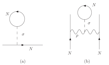
Figure 7: Walecka mean field contribution of the scalar tadpole to the nucleon mass (a) and its extrapolation to constituent quarks in vector mesons (b).

A number of previous studies friman2 ; song1 ; song2 were successful in describing nuclear matter by starting from a chiral Lagrangian with nuclear, scalar, and vector degrees of freedom in which the hadronic masses were scaled with density according to (32). In particular, the compression modulus and anomalous orbital gyromagnetic ratio were found to be in excellent agreement with experiment, which suggests that a similar approach may prove fruitful in our present analysis. An alternative approach, complementary to the chiral Lagrangian method, is to include medium modifications directly into a one-boson-exchange potential. Such a calculation was carried out in rapp to study the saturation of nuclear matter. In their work it was suggested that the $\sigma$ particle should be constructed microscopically as a pair of correlated pions interacting largely through crossed-channel $\rho$ exchange. Medium modifications to the $\sigma$ mass then arises naturally from the density-dependence of the $\rho$ mass. The final conclusion established in rapp is that at low densities the $\sigma$ scales according to (32) but that toward nuclear matter density the scaling is slowed to such an extent that saturation can be achieved.

We proceed along the lines of rapp and introduce medium modifications directly into a one-boson-exchange potential. The most refined NN potentials in this category are the Nijmegen I, Nijmegen II, and CD-Bonn potentials. The Nijmegen potentials include contributions from the exchange of $\rho,\omega,\phi,\sigma,f_{0},$ and $a_{0}$ mesons, as well as the pseudoscalar particles which do not receive medium modifications in Brown-Rho scaling. The CD-Bonn potential includes two vector particles (the $\rho$ and $\omega$) and two scalars ($\sigma_{1}$ and $\sigma_{2}$). For both potentials we scale the vector meson masses by 15% and the scalar meson masses by 7%. In this way we roughly account for the decreased scaling of the scalar particle mass observed in rapp . In the full many-body calculation we also scale the nucleon mass by 15% and with an additional $\sqrt{g_{A}^{*}/g_{A}}\simeq 1/\sqrt{1.25}$ at nuclear matter density. It is essential to also scale the form factor cutoffs $\Lambda_{f}$ of the vector mesons in the boson-exchange potentials.

In Table 4 we show the effective mass, compression modulus, symmetry energy, and anomalous orbital gyromagnetic ratio for the Nijmegen I & II and CD-Bonn potentials with the in-medium modifications. We also show for comparison the results from the Nijmegen93 one-boson-exchange potential, which has only 15 free parameters and is not fine-tuned separately in each partial wave. We observe that the iterative solution is in better agreement with all nuclear observables. The anomalously large compression modulus in the CD-Bonn potential results almost completely from the presence of a large $\omega$ coupling constant $g_{\omega NN}^{2}/4\pi=20.0$. With the same $g_{\omega NN}^{2}/4\pi$ and Bonn-B potential, Rapp et al. rapp obtained ${\cal K}=356$ MeV. The compression modulus is very sensitive to this parameter, as we have checked that dropping this coupling by 20% cuts the compression modulus in half but alters the other nuclear observables by less than 5%. The naive quark model predicts a ratio of $g_{\omega NN}^{2}/g_{\rho NN}^{2}=9$ between the $\omega$ and $\rho$ coupling constants, which is largely violated in the CD-Bonn potential $g_{\omega NN}^{2}/g_{\rho NN}^{2}=24$ though roughly satisfied in the Nijmegen potentials $g_{\omega NN}^{2}/g_{\rho NN}^{2}=11$, perhaps resulting in better agreement with experiment.

Thus, by extension of the Walecka mean field on nucleons to those on constituent quarks, we obtain the Fermi liquid parameters for the theory that is now essentially Brown-Rho scaled, as shown in Table 5. One should note that these results are only for infinite nuclear matter and especially the three-body term will act in many different diagrams in the finite systems. However, our arguments suggest that the three-body terms intrinsic to Brown-Rho scaling will be useful in stabilizing light nuclei.

	$V_{\rm NI}$	$V_{\rm NII}$	$V_{N93}$	$V_{\rm CDB}$
$m^{*}/m$	0.721	0.763	0.696	0.682
${\cal K}$ [MeV]	218	142	190	495
$\beta$ [MeV]	20.4	25.5	23.7	19.2
$\delta g_{l}$	0.246	0.181	0.283	0.267

Table 4: Nuclear observables obtained from the self-consistent solution to the Babu-Brown equations incorporating Brown-Rho scaling. Four different bare potentials – the CD-Bonn potential ($V_{\rm CDB}$), Nijmegen I ($V_{\rm NI}$), Nijmegen II ($V_{\rm NII}$), and Nijmegen93 ($N93$) potentials – were used to construct low momentum interactions for a cutoff of $\Lambda=2.1$ fm^-1. In eq. (32) the parameter $C=0.15$.

$l$	$F_{l}$	$G_{l}$	$F^{\prime}_{l}$	$G^{\prime}_{l}$
0	-0.20 $\pm$ 0.39	0.04 $\pm$ 0.11	0.24 $\pm$ 0.16	0.53 $\pm$ 0.09
1	-0.86 $\pm$ 0.10	0.19 $\pm$ 0.06	0.18 $\pm$ 0.05	0.17 $\pm$ 0.12
2	-0.21 $\pm$ 0.01	0.12 $\pm$ 0.01	0.10 $\pm$ 0.02	0.01 $\pm$ 0.02
3	-0.09 $\pm$ 0.01	0.05 $\pm$ 0.01	0.05 $\pm$ 0.01	0.01 $\pm$ 0.01

Table 5: Fermi liquid coefficients for the self-consistent solution to the Babu-Brown equations using Brown-Rho scaled nucleon and meson masses in the four low momentum CD-Bonn and Nijmegen potentials listed in Table 4. The tabulated values display the average and spread from the four different potentials and not the actual uncertainties associated with the Fermi liquid parameters.

V Discussion of the tensor force with dropping $\rho$-mass in saturation of nuclear matter

The tensor force contributes chiefly in second order perturbation theory as an effective central force in the $I=1$ channel. As the density increases, some of the intermediate states are blocked by the Pauli principle. In the two-body system the tensor force contributes to the ${}^{3}S_{1}$ state, but not to the ${}^{1}S_{0}$ state, and gives most of the attractive interaction difference between the ${}^{3}S_{1}$ and ${}^{1}S_{0}$ states, effectively binding the deuteron. However, the intermediate state energies relevant for the second-order tensor force are $>225$ MeV (See Fig. 69 of brown3 which is for ⁴⁰Ca. For nuclear matter the intermediate state momenta would be higher.), well above the Fermi energy of nuclear matter, and most intermediate momenta are above the $V_{{\rm low}-k}$ upper model space limit of 420 MeV/c, so the tensor force is largely integrated out.

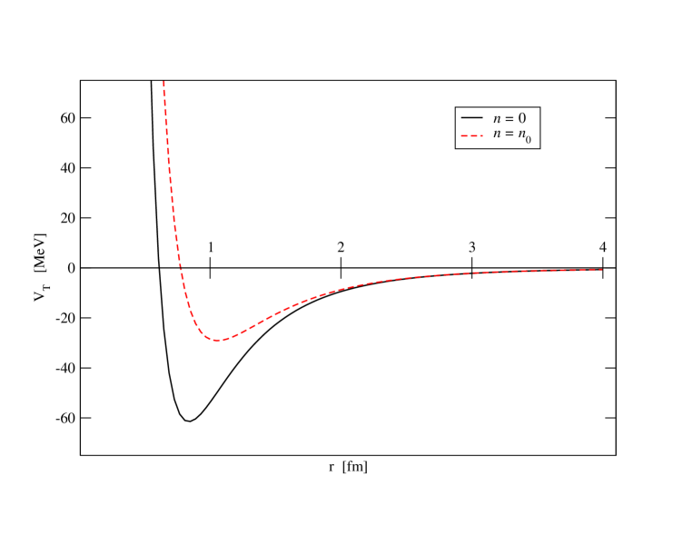
Figure 8: Reduction in the strength of the tensor force due to a scaled $\rho$-meson mass. Contributions from both $\pi$-meson and $\rho$-meson exchange are included in both curves. We have used the Brown-Rho parametric scaling, so that at nuclear matter density $m^{*}_{\rho}=0.8m_{\rho}$.

However, since the beginning of Brown-Rho scaling it has been understood that the tensor force is rapidly cut down with increasing density. That is because the pion mass does not change with density, being protected by chiral invariance, but the $\rho$-meson mass, which is dynamically generated, decreases by 20% (parametric scaling) in going from a density of $n=0$ to nuclear matter density $n=n_{0}$. Since the $\rho$-meson exchange contributes with opposite sign from that of the pion, this cuts down the tensor force substantially. In Fig. 8 we show the total tensor force from $\pi$ and $\rho$ exchange at zero density and nuclear matter density $n_{0}$. Since it enters in the square, this means a factor of several drop in the tensor contribution to the binding energy, as shown in Fig. 9.

We believe that the work of ref. trnka shows unambiguously that the mass of the $\omega$-meson is $\sim$ 14% lower at nuclear matter density than in free space. It is remarkable that nuclear structure calculations have been carried out for many years without density-dependent masses but with results usually in quantitative agreement with experiment. In brown5 Brown and Rho showed that in cases where the exchange of the $\pi$-meson is not important, such as in Dirac phenomenology, there is a scale invariance such that if the masses of all relevant mesons are changed by the same amount, the results for the physical phenomena are very little changed.

Since the pion exchange gives the longest range part of the nucleon-nucleon interaction, it is amazing that there are not clearcut examples in nuclear spectroscopy such as level orderings that are altered by the $\rho$-meson exchange playing counterpoint to the $\pi$-meson exchange, as we find in this paper for nuclear saturation. The in-medium decrease in the $\rho$-mass increases the effect of $\rho$-exchange, which enters so as to cut down the overall tensor force, the $\rho$ and $\pi$ exchange entering with opposite sign.

Finally, nearly forty years since the Kuo-Brown nucleon-nucleon forces were first published, it was shown holt1 that the summation of core polarization diagrams to all orders is well-approximated by a single bubble. However, in light of the double decimation of brown5 being carried out here in one step, these forces should be modified to include the medium dependence of the masses. Phenomenologically this can be done by introducing three-body terms, as we did here, but from our treatment of the second-order tensor force it is clear that this should be done at constituent quark level.

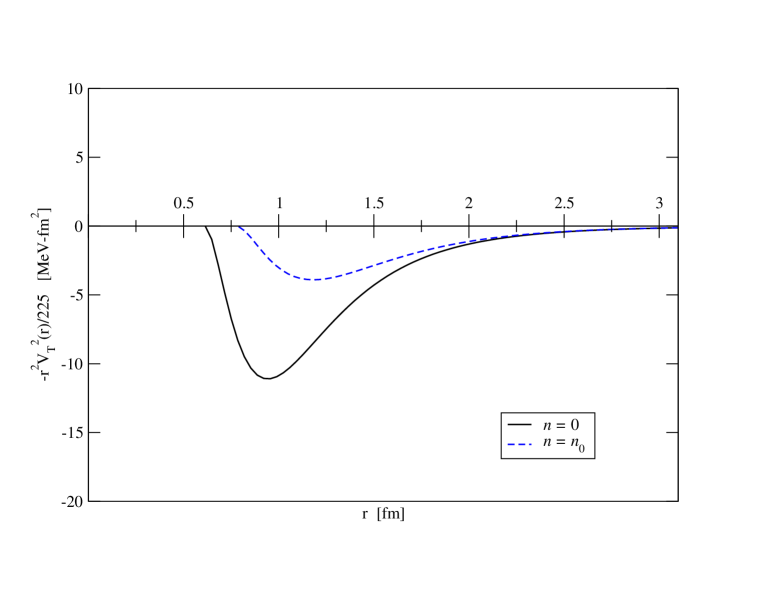
Figure 9: Reduction of the tensor force in second order perturbation theory due to a scaled $\rho$-meson mass. The intermediate state energy is approximated as 225 MeV. Contributions from both $\pi$-meson and $\rho$-meson exchange are included in both curves. At nuclear matter density, $n_{0}$, we have used the parametric scaling $m^{*}_{\rho}=0.8m_{\rho}$.

VI Conclusion

We believe that by discussing the nuclear many-body problem within the context of Fermi liquid theory with the interaction $V_{{\rm low}-k}$ following the work of Schwenk et al. schwenk1 we have a format for understanding connections between the physical properties of the many-body system and the nuclear potentials. We carried out an iterative solution of the Babu-Brown equations, which include both density-density and current-current correlation functions, calculating input potentials via a momentum space decimation to $V_{{\rm low}-k}$. By including Brown-Rho scaling through scalar tadpoles, as suggested by Walecka theory, our iterative solution provides the empirical Fermi liquid quantities. Our nucleon effective mass is on the low side of those usually employed, as is common in Walecka mean field theory.

- (1) G. E. Brown and M. Rho, Phys. Rept. 396 (2004) 1.
- (2) L. D. Landau, Sov. Phys. JETP, 3 (1957) 920.
- (3) L. D. Landau, Sov. Phys. JETP, 5 (1957) 101.
- (4) L. D. Landau, Sov. Phys. JETP, 8 (1959) 70.
- (5) A. B. Migdal and A. I. Larkin, Sov. Phys. JETP 18 (1964) 717.
- (6) A. B. Migdal, Theory of Finite Fermi Systems and Applications to Atomic Nuclei (Interscience, New York, 1967).
- (7) S. O. Bäckman, Nucl. Phys. A120 (1968) 593; A130 (1969) 481.
- (8) G. E. Brown, Rev. Mod. Phys. 43 (1971) 1.
- (9) R. S. Poggioli and A. D. Jackson, Nucl. Phys. A165 (1971) 582.
- (10) S. K. Bogner, T. T. S. Kuo, and A. Schwenk, Phys. Rept. 386 (2003) 1.
- (11) A. Schwenk, G. E. Brown, and B. Friman, Nucl. Phys. A703 (2002) 745.
- (12) A. Schwenk, B. Friman, and G. E. Brown, Nucl. Phys. A713 (2003) 191.
- (13) A. Schwenk and B. Friman, Phys. Rev. Lett. 92 (2004) 082501.
- (14) J. Kuckei, F. Montani, H. Muther, A. Sedrakian, Nucl. Phys. A 723 (2003) 32.
- (15) S. K. Bogner, A. Schwenk, R. J. Furnstahl, and A. Nogga, Nucl. Phys. A763 (2005) 59.
- (16) S. Babu and G.E. Brown, Ann. Phys. 78 (1973) 1.
- (17) O. Sjöberg, Ann. Phys. 78 (1973) 39.
- (18) O. Sjöberg, Nucl. Phys. A209 (1973) 363.
- (19) W. H. Dickhoff, A. Faessler, H. Müther, and S. S. Wu, Nucl. Phys. A405 (1983) 534.
- (20) S. O. Bäckman, G. E. Brown, and J. A. Niskanen, Phys. Rept. 124 (1985) 1.
- (21) K. S. Bedell and T. L. Ainsworth, Phys. Lett. A102 (1984) 49.
- (22) G. E. Brown and M. Rho, Phys. Rev. Lett. 66 (1991) 2720.
- (23) T. T. S. Kuo and G. E. Brown, Nucl. Phys. 85 (1966) 40.
- (24) I. Ya. Pomeranchuk, Zh. Eksperim. Teor. Fiz. 35 (1958) 524.
- (25) A. A. Abrikosov, L. P. Gorkov, and I. E. Dzyaloshinki, Methods of Quantum Field Theory in Statistical Physics (Dover, New York, 1963).
- (26) F. Nozieres, Theory of Interacting Fermi Systems (Addison-Wesley, Reading, Massachusetts, 1964).
- (27) B. L. Friman and A. K. Dar, Phys. Lett. B 85 (1979) 1.
- (28) G. E. Brown, Many-Body Problems (North-Holland, Amsterdam, 1972).
- (29) S. K. Bogner, T. T. S. Kuo, A. Schwenk, D. R. Entem, and R. Machleidt, Phys. Lett. B576 (2003) 265.
- (30) R. B. Wiringa, V. G. J. Stoks, and R. Schiavilla, Phys. Rev. C 51 (1995) 38.
- (31) R. Machleidt, Phys. Rev. C 63 (2001) 024001.
- (32) V. Pandharipande, I. Sick, and P. de Witt Huberts, Rev. Mod. Phys. 69 (1997) 981.
- (33) D. H. Youngblood, H. L. Clark, and Y.-W. Lui, Phys. Rev. Lett. 82 (1999) 691.
- (34) A. W. Steiner, M. Prakash, J. M. Lattimer, and P. J. Ellis, Phys. Rept. 411 (2005) 325.
- (35) P. Möller, J. R. Nix, W. D. Myers, and W. J. Swiatecki, Atom. Data and Nucl. Data Tabl. 59 (1995) 185.
- (36) P. Danielewicz, Nucl. Phys. A727 (2003) 233.
- (37) R. Nolte, A. Baumann, K. W. Rose, and M. Schumacher, Phys. Lett. B 173 (1986) 388.
- (38) G. E. Brown and Mannque Rho, Phys. Rept. 269 (1996) 333.
- (39) D. Trnka et al., Phys. Rev. Lett. 94 (2005) 192303.
- (40) M. Naruki et al., Phys. Rev. Lett. 96 (2006) 092301.
- (41) M. Harada, Y. Kim, and M. Rho, Phys. Rev. D 66 (2002) 016003.
- (42) B. Friman and M. Rho, Nucl. Phys. A606 (1996) 303.
- (43) C. Song, G. E. Brown, D.-P. Min, and M. Rho, Phys. Rev. C 56 (1997) 2244.
- (44) C. Song, Phys. Rept. 347 (2001) 289.
- (45) R. Rapp, R. Machleidt, J. W. Durso, and G. E. Brown, Phys. Rev. Lett. 82 (1999) 1827.
- (46) G. E. Brown, Unified Theory of Nuclear Models and Forces (North-Holland, Amsterdam, 1967).
- (47) J. D. Holt, J. W. Holt, T. T. S. Kuo, G. E. Brown, and S. K. Bogner, Phys. Rev. C 72 (2005) 041304(R).