$\omega-\pi\gamma^{*}$ transition form factor in proton-proton collisions

Abstract

Dalitz decays of $\omega$ and $\rho$ mesons, $\omega\to\pi^{0}\gamma^{*}\to\pi^{0}e^{+}e^{-}$ and $\rho^{0}\to\pi^{0}\gamma^{*}\to\pi^{0}e^{+}e^{-}$, produced in $pp$ collisions are calculated within a covariant effective meson-nucleon theory. We argue that the $\omega$ transition form factor $F_{\omega\to\pi^{0}\gamma^{*}}$ is experimentally accessible in a fairly model independent way in the reaction $pp\to pp\pi^{0}e^{+}e^{-}$ for invariant masses of the $\pi^{0}e^{+}e^{-}$ subsystem near the $\omega$ pole. Numerical results are presented for the intermediate energy kinematics of envisaged HADES experiments.

I Introduction

The investigation of vector meson production in nucleon-nucleon ($NN$) reactions represents an interesting topic with various implications. For instance, it is known that the effective repulsive $NN$ forces at short distances can be described, within a boson exchange model, by the exchange of $\rho$ and $\omega$ mesons so that a study of their contribution to the $NN$ elastic amplitude and to the meson exchange currents in elastic scattering processes off light nuclei can substantially augment the knowledge of the short-range part of the $NN$ potential. Another important issue of vector meson production in $NN$ collisions is related to electromagnetic probes of strongly interacting systems. As vector mesons carry the $J^{P}=1^{-}$ quantum numbers as the photon, they couple directly to real and virtual photons. The latter ones can be converted into di-electrons in an $s$-channel process, such allowing a direct access to the spectral distribution of the parent vector meson, even when embedded in strongly interacting matter. (The strong decay channel products would suffer from final state interaction with the ambient medium. Thus, the di-electron channel serves as direct or penetrating probe Rapp_Wambach .)

Furthermore, the decay $\omega\to\pi^{0}\gamma$ was recently experimentally studied in photo-excitation of nuclei CB_TAPS . The difference of the strength distribution of the parent $\omega$ for different target nuclei has been ascribed to a medium modification our_PRL . Such medium modifications are of particular importance for understanding the electromagnetic emissivities of highly excited, strongly interacting systems, e.g., created in the course of relativistic heavy-ion collisions. An extreme option is that the resonances, including the $\rho$ and $\omega$ mesons, are molten once the deconfinement and chirally restored phase is entered our_em_papers .

Another aspect is to supply information on production of vector mesons in nucleon-nucleon reactions with similar quantum numbers but rather different quark content, such as $\omega$ and $\phi$ mesons ourOmega ; ourPhi ; nakayama ; sibir , which is interesting with respect to the Okubo-Zweig-Iizuka rule ozi and hidden strangeness in the nucleon.

A particularly interesting subject is the decay of a vector meson. Besides the above mentioned direct di-electron decay, $V\to e^{+}e^{-}$, where $V$ stands generically for a vector meson, valuable information on the half-off-mass shell decay vertex $V\to\pi\gamma^{*}\to\pi e^{+}e^{-}$ and related transition form factors (FF) can be obtained. The functional dependence of FF’s upon the momentum transfer encodes general characteristics of hadrons, such as charge and magnetic distributions, size etc. The mentioned $\omega$ transition FF is related to the ratio of matrix elements $\langle\omega|\pi^{0}\gamma^{*}\rangle/\langle\omega|\pi^{0}\gamma\rangle$.

FF’s are also known as important objects for studying bound states within non-perturbative QCD. Theoretical tools for exclusive processes within non-perturbative QCD are approaches based on light cone sum rules and factorization theorem (see rad1 ; rad ; novikov ; isgur ; isgur1 and references therein).

In deep-inelastic scattering processes, an investigation of FF’s in a large interval of momentum transfer, including the time-like region, serves as an important tool to provide additional information about the various QCD regimes and on the interplay between soft and hard contributions. For instance, it has been found that the soft part can be treated as contribution of configurations in the Fock space with a minimal number of quark constituents. This can be considered as a justification for approaches based on the relativistic quark constituent model for a covariant treatment of mesons as two-particle bound states (see refs. moris ; anisovich_BS for details of covariant description of mesons within Bethe-Salpeter like approaches); correspondingly computed FF’s serve as tests of models fred ; salme ; moris ; anisovich_BS ; anisovich_IE ; anisovich_FF .

Besides the mentioned QCD-motivated approaches there is a number of more phenomenological models, e.g., based on the dispersion relation technique anisovich_IE ; omegaFormfNormaliz , or on the use of vector meson dominance (VMD) models faessler ; thomas ; meissner or with effective SU(3) chiral Lagrangians with inclusion of the non-Abelian anomaly meissner ; kaiser ; nonAbelian .

Traditionally, the electromagnetic FF’s are studied by electron scattering off stable particles which provides information in the space-like region of momenta where, as well known, the experimental data can be peerless parameterized by dipole formulae. This in turn means that in the unphysical region, i.e., for kinematics unreachable by experiments with on-mass shell particles, the analytically continued FF’s exhibit a pole structure. Intensively studied FF’s are the ones of the pseudoscalar mesons, chiefly the pion. Light vector meson FF’s have received less attention since their experimental determination is more difficult. However, new detector installations, like the spectrometer HADES HADES , can detect di-electrons production in proton-proton ($pp$) collisions in a wide kinematical range of invariant masses with a high efficiency. Thus, a precision study of the transition FF for the $\omega\to\pi^{0}e^{+}e^{-}$ process becomes feasible.

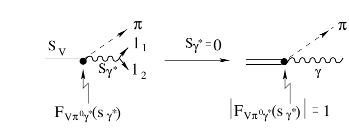
Figure 1: Left part: Dalitz decay of a vector meson with energy squared $s_{V}$ into a pion ($\pi$) and a di-electron ($l_{1},l_{2}$). Right part: the transition form factor is normalized at the photon point, i.e., $\left|F_{V\pi^{0}\gamma^{*}}(S_{\gamma^{*}=0})\right|=1$.

The process of vector meson Dalitz decay can be presented as (see Fig. 1)

$$V\to P+\gamma^{*}\to P+e^{-}+e^{+}$$ (1)

where $P$ denotes a pseudoscalar meson. Obviously, the probability of emitting a virtual photon is governed by the dynamical electromagnetic structure of the ”dressed” transition vertex $V\to P$ which is encoded in the transition FF’s. If the particles $V$ and $P$ were point like, then calculations of mass distributions and decay widths would be straightforward along the standard quantum electrodynamics (QED) technique. Deviations of the measured quantities from the QED predictions directly reflect the effects of the FF’s and thus the internal hadron structure, and, consequently, can serve as experimental tests to discriminate the different theoretical approaches.

First experimental measurements of the $\omega$ transition FF LandPhysRep ; omegaFrmf1 ; omegaFrmf2 ; omegaFrmf3 have pointed to a discrepancy with theoretical pre(post)dictions omegaFormfNormaliz ; moris ; kaiser in the time-like region. Calculations based on VMD do not satisfactorily describe the data. A better description can be achieved with dispersion relation calculations omegaFormfNormaliz or within models based on the Dyson-Schwinger equation moris . All these approaches provide rather different transition FF’s, with the difference increasing with the momentum transfer. However, the available experimental data is still too scarce for a preferable choice of the approach, and additional data is needed. In this context, forthcoming data from the HADES collaboration at the heavy ion synchrotron SIS18/GSI Darmstadt HADES will substantially contribute to our understanding of the problem.

HADES is a detector installation optimized for studies of processes with a $e^{+}e^{-}$ pair in one of the final states in reactions of hadrons $(p,\pi$) and various nuclei, i.e., $pp$, $\pi p$, $Dp$, $pA$, $\pi A$, $AA$ etc. near the $\rho$, $\omega$ and $\phi$ thresholds. In the present paper we study the di-electron production from Dalitz decay of the lightest vector mesons in $pp$ reactions at beam energies of a few GeV for kinematical conditions corresponding to the HADES setup. Our focus is to investigate the transition FF $\omega\to\pi^{0}e^{+}e^{-}$. To this end we calculate the dependence of the differential cross section for the reaction $pp\to pp\pi^{0}e^{+}e^{-}$ upon the invariant mass of the subsystem $\pi^{0}e^{+}e^{-}$ around the pole masses of $\rho$ and $\omega$ mesons and find a kinematical range where the contribution of $\rho$ is sufficiently small and the cross section is dominated by Dalitz decays of $\omega$ mesons. We calculate the double differential cross section averaged in a suitable kinematical range as a function of the di-electron invariant mass and argue that such a quantity, normalized to the real photon point and supplemented by some specific kinematical factor, represents the desired transition FF. In such a way a direct experimental investigation of the $\omega$ transition FF is feasible.

Our paper is organized as follows. In section 2 we introduce the $\omega\to\pi^{0}\gamma^{*}$ transition form factor. Section 3 is devoted to the theoretical background for dealing with the reactions $pp\to pp\omega\to pp\pi^{0}e^{+}e^{-}$ and$pp\to pp\rho\to pp\pi^{0}e^{+}e^{-}$. Numerical results are presented in section 4. The conclusions are summarized in section 5, and some formal relations for an integration procedure are relegated to the appendix.

II The transition form factor

Consider the process of a Dalitz decay of a vector meson into a pion and a virtual photon (di-electron) of the type (1). The effective Lagrangian describing the vertex $V\to\pi^{0}\gamma$ reads meissner ; thomas ; anisovich_FF

$${\cal L}_{V\pi^{0}\gamma}=f_{V\pi^{0}\gamma}\ \left(\epsilon_{\mu\nu\alpha\beta}\partial^{\mu}A^{\nu}\partial^{\alpha}\Phi_{V}^{\beta}\right){\mathchar 28680\relax}_{\pi}^{0},$$ (2)

where $A^{\nu}$ is the electromagnetic four-potential, $\Phi_{V}$ denotes the neutral vector meson fields $\omega$ or $\rho$, respectively, ${\mathchar 28680\relax}_{\pi}^{0}$ stands for the $\pi^{0}$ part of the isovector ${\mathchar 28680\relax}_{\pi}$ pion field, and $f_{V\pi^{0}\gamma\,}$ is the corresponding coupling constant. The decay width is calculated from (2) as

$$\Gamma_{V\to\pi^{0}\gamma}=\frac{1}{12\pi}\left(\frac{\lambda(s_{V},0,\mu_{\pi}^{2})}{4s_{V}}\right)^{3/2}f_{V\pi^{0}\,\gamma}^{2}$$ (3)

and serves for a determination of the coupling constant $f_{V\pi^{0}\,\gamma}$ from experimental data. $\lambda$ is the kinematical triangle function, $\lambda(x,y,z)=(x-(\sqrt{y}-\sqrt{z})^{2})(x-(\sqrt{y}+\sqrt{z})^{2})$ and the square of the $\pi^{0}\gamma$ invariant mass is denoted by $s_{V}$. Experimentally, the branching ratios ${\Gamma_{i}}/{\Gamma_{tot}}$ for $\omega\to\pi^{0}\gamma$ and $\rho\to\pi^{0}\gamma$ are known, being $\left(8.9^{+0.27}_{-0.23}\right)\cdot 10^{-2}$ and $\left(6.1\pm 0.8\right)\cdot 10^{-4}$ dataGroup . Eq. (3) yields $f_{\omega\pi^{0}\gamma\,}\simeq 0.72\ \ GeV^{-1}$ and $f_{\rho\pi^{0}\gamma\,}\simeq 0.25\ \ GeV^{-1}$ for the known total widths $\Gamma_{\omega}=(8.49\pm 0.08)\ MeV$ and $\Gamma_{\rho}=(146.5\pm 1.5)\ MeV$. For the reaction (1), however, the emitted photon is virtual and, consequently, the Lagrangian (2) must be supplemented by including the corresponding transition FF $V\to P$. Then, for the $\omega$ meson one has

$$\frac{d\Gamma}{ds_{\gamma^{*}}}=\left(\displaystyle\frac{d\Gamma}{ds_{\gamma^{*}}}\right)_{\rm point}\left|F_{\omega\pi^{0}{\gamma^{*}}\,}(s_{\gamma^{*}})\right|^{2},$$ (4)

where $s_{\gamma^{*}}$ is the di-electron invariant mass squared. Formally, eq. (4) can be considered as the definition of the transition form factor. Direct calculation of the diagram Fig. 1 with the Lagrangian (2) results in

$$\displaystyle\frac{d\Gamma_{\omega\to\pi^{0}e^{+}e^{-}}}{ds_{\gamma^{*}}}=\displaystyle\frac{\alpha_{em}}{3\pi s_{\gamma^{*}}}\frac{\lambda^{3/2}(s_{V},s_{\gamma^{*}},\mu_{\pi}^{2})}{\lambda^{3/2}(s_{V},0,\mu_{\pi}^{2})}\Gamma_{\omega\to\pi^{0}\gamma}\left|F_{\omega\pi^{0}\gamma^{*}\,}(s_{\gamma^{*}})\right|^{2}.$$ (5)

The mass distribution $\displaystyle\frac{d\Gamma_{\omega\to\pi^{0}e^{+}e^{-}}}{ds_{\gamma^{*}}}$ is determined by (i) a purely kinematical (calculable) factor, (ii) the decay vertex into a real photon (known from experimental data) and (iii) the (yet poorly known) transition FF $F_{\omega\pi^{0}\gamma^{*}\,}(s_{\gamma^{*}})$. Hence, eq. (5) demonstrates that by measuring the invariant mass distribution one can get direct experimental access to the $\omega$ transition FF LandPhysRep ; omegaFrmf1 ; omegaFrmf2 ; omegaFrmf3 .

As mentioned above, the transition FF’s are important objects of theoretical calculations for tests and discrimination among the multitude of approaches. The simplest and quite successful theoretical description of FF’s can be performed faessler ; meissner ; kaiser within the VMD conjecture, and a reasonably good description of elastic FF’s in the time-like region has been accomplished. By using the current-field identity meissner

$$J^{\mu}=-e\frac{M_{\rho}^{2}}{f_{\gamma\rho}}\Phi_{\rho^{0}}^{\mu}-e\frac{M_{\omega}^{2}}{f_{\gamma\omega}}\Phi_{\omega}^{\mu}$$ (6)

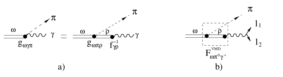
Figure 2: Diagrams for calculation of the transition form factor $F_{\omega\pi\gamma}(s_{\gamma^{*}})$ within the VMD model. Diagrams in a) correspond to the current-field identity (6), while diagram b) is the Dalitz decay within the VMD model.

with the coupling constants $f_{\gamma\rho}$ and $f_{\gamma\omega}$ known friman1 ; friman2 from experimentally measured electromagnetic decay widths, one can also compute the transition form factor $F^{VMD}_{\omega\pi^{0}\gamma^{*}\,}(s_{\gamma^{*}})$ by evaluating the corresponding Feynman diagrams (see fig. 2). Contrarily to the elastic case, the FF computed within such an approach exhibits disagreement with data (see below). This immediately implies that with only one (local) FF it is not possible to satisfactorily describe kaiser ; friman2 the transition vertex, and the simple $\rho/\omega$ dominance model must be, at least phenomenologically, supplemented with heavier mesons to modify appropriately the shape of the transition vertex faessler .

III The reaction $\bf pp\to pp{\mbox{\boldmath$\pi$}}^{0}e^{+}e^{-}$

Consider now the di-electron ($e^{+}e^{-}$) production in the exclusive reaction

$$N_{1}+N_{2}\to N_{1}^{\prime}+N_{2}^{\prime}+\pi^{0}+e^{+}+e^{-}$$ (7)

for which the process (1) enters as a subreaction. The invariant cross section is

$$d^{11}\sigma=\frac{1}{2\sqrt{\lambda(s,m^{2},m^{2})}}\frac{1}{(2\pi)^{11}}\frac{1}{4}\sum\limits_{\rm spins}\ \,|\ T(P_{1}^{\prime},P_{2}^{\prime},k_{1},k_{2},k_{\pi},{\rm spins})\ |^{2}d^{11}\tau_{f}\ \frac{1}{n!},$$ (8)

where the factor $1/n!$ accounts for $n$ identical particles in the final state, $|T|^{2}$ denotes the invariant amplitude squared, and the invariant phase volume $d\tau_{f}$ is

$$d^{11}\tau_{f} = ds_{12}ds_{V}ds_{\gamma^{*}}\,R_{2}(P_{1}+P_{2}\to P_{V}+P_{12})R_{2}(P_{12}\to P_{1}^{\prime}+P_{2}^{\prime})$$ (9)

$$\times R_{2}(P_{V}\to k_{\pi}+P_{\gamma})\ R_{2}(P_{\gamma}\to k_{1}+k_{2})$$

with the two-body invariant phase space volume $R_{2}$ defined as

$$R_{2}(a+b\to c+d)=d^{4}P_{c}\ d^{4}P_{d}\ \delta^{(4)}\left(P_{a}+P_{b}-P_{c}-P_{d}\right)\delta\left(P_{c}^{2}-m_{c}^{2}\right)\ \delta\left(P_{d}^{2}-m_{d}^{2}\right),$$ (10)

where $P_{1},P_{2}$ and $P_{1}^{\prime},P_{2}^{\prime},k_{1},k_{2},k_{\pi}$ are the four-momenta of the initial and final particles, respectively; $m$ denotes the nucleon mass, while the electron mass can be neglected for the present kinematics. The invariant mass of two particles is hereafter denoted as $s$. The invariant phase volume $d\tau_{f}$ in (9) has been chosen within the so-called ”duplication” kinematics bykling , i.e. the one which exploits invariant two-dimensional phase volumes $R_{2}$ describing (kinematically) the decay of a real or virtual particle with the invariant mass squared $s$ into two particles, which can also be either real or virtual. This kinematics is schematically depicted in Fig. 3.

The invariant amplitude $T$ is evaluated here within a phenomenological meson-nucleon theory based on effective interaction Lagrangians which include scalar ($\sigma$), pseudoscalar ($\pi$), and neutral ($\omega$) and charged/neutral vector ($\rho$) mesons (see nakayama ; nakayama1 ; ourPhi ; ourOmega ; ourNuclPhys ; titov )

$${\cal L}_{NN\sigma} = g_{\sigma}\bar{N}N\it\Phi_{\sigma},$$ (11)

$${\cal L}_{NN\pi} = -\frac{f_{NN\pi}}{m_{\pi}}\bar{N}\gamma_{5}\gamma^{\mu}\partial_{\mu}({{\mathchar 28956\relax}{\mathchar 28680\relax}_{\pi}})N,$$ (12)

$${\cal L}_{NN\rho} = -g_{NN\rho}\left(\bar{N}\gamma_{\mu}{{\mathchar 28956\relax}}N{{\mathchar 28680\relax}_{\rho}}^{\mu}-\frac{\kappa_{\rho}}{2m}\bar{N}\sigma_{\mu\nu}{{\mathchar 28956\relax}}N\partial^{\nu}{{\mathchar 28680\relax}_{\rho}}^{\mu}\right),$$ (13)

$${\cal L}_{NN\omega} = -g_{NN\omega}\left(\bar{N}\gamma_{\mu}N{\it\Phi}_{\omega}^{\mu}-\frac{\kappa_{\omega}}{2m}\bar{N}\sigma_{\mu\nu}N\partial^{\nu}\it\Phi_{\omega}^{\mu}\right),$$ (14)

where $N$ and $\it\Phi$ denote the nucleon and meson fields, respectively, and bold face letters stand for isovectors. All couplings with off-mass shell particles are dressed by monopole form factors $F_{M}=\left(\Lambda^{2}_{M}-\mu_{M}^{2}\right)/\left(\Lambda^{2}_{M}-k^{2}_{M}\right)$, where $k^{2}_{M}$ is the four-momentum of a virtual particle with mass $\mu_{M}$. At $\rho$/$\omega$ threshold-near kinetic energies, contributions from heavier mesons ($\phi$, $a_{1}$ …) can be neglected, and we consider first only the Dalitz decays of $\rho$ and $\omega$ mesons.

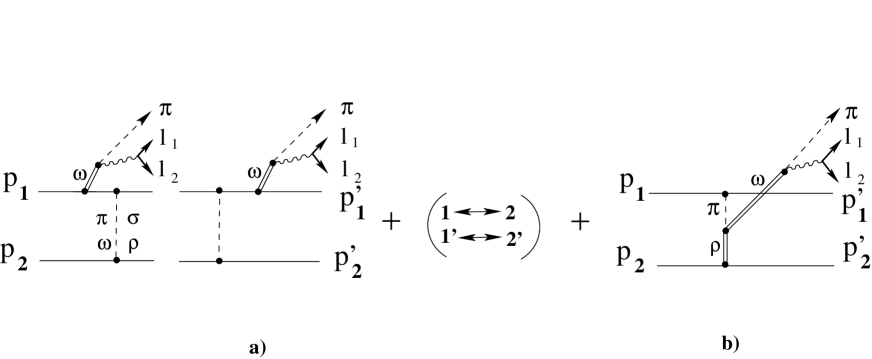
Figure 4: Diagrams for the resonant part of the process $NN\to NN+\pi+e^{+}e^{-}$ within an effective meson-nucleon theory with Lagrangians defined by eq. (14). a) Dalitz decay of $\omega$ meson from bremsstrahlung diagrams, b) Dalitz decay of $\omega$ mesons from internal conversion. Analogous diagrams hold for the $\rho$ meson.

The Lagrangians (11 - 14) generate two classes of Feynman diagrams: (i) the ones which describe the Dalitz decay of a vector meson created from nucleon bremsstrahlung due to $NN$ interaction (via a one-boson exchange potential), see Fig. 4a, and (ii) Dalitz decay of a vector meson, $\omega$ or $\rho$, from a conversion of virtual $\pi$ and $\rho$ (or $\pi$ and $\omega$) exchange bosons into an intermediate vector meson, i.e., from the internal $\rho\pi\omega$ vertex, see Fig. 4b. The result of a calculation of these diagrams can be cast in the form of a current-current interaction

$$T=J_{\alpha}(12\to 1^{\prime}2^{\prime}V)\left(\displaystyle\frac{g^{\alpha\beta}-\frac{P_{V}^{\alpha}P_{V}^{\beta}}{P_{V}^{2}}}{P_{V}^{2}-M_{V}}\frac{e\,f_{V\pi^{0}\gamma\,}}{P_{\gamma}^{2}}\right)\left(\epsilon_{\mu\nu\beta\beta^{\prime}}P_{\gamma^{*}}^{\mu}P_{V}^{\beta^{\prime}}j_{\pm}^{\nu}\right),$$ (15)

where $j_{\pm}^{\nu}=\bar{u}(k_{1})\gamma^{\mu}v(k_{2})$ is the electromagnetic current of the final lepton pair, and $J_{\alpha}(12\to 1^{\prime}2^{\prime}V)$ stands for the current corresponding to the vector meson production in $NN$ interaction, i.e., the Feynman diagrams $NN\to NNV$ ourOmega with the vector meson lines truncated (cf. Fig. 4).

The amplitude $T$ consists of two parts: one ($J_{\alpha}(12\to 1^{\prime}2^{\prime}V)$) describing the production of vector mesons, and the other one $\left(\epsilon_{\mu\nu\beta\beta^{\prime}}P_{\gamma^{*}}^{\mu}P_{V}^{\beta^{\prime}}j_{\pm}^{\nu}\right)$ being proportional to the amplitude of Dalitz decays of the produced mesons. This prominent feature of the amplitude allows to substantially simplify the expression for the cross section. In the square of the amplitude one can separate groups of terms which depend only on a part of variables (connected with decay vertices), and correspondingly the multidimensional integral (8) can be partially factorized. Note that the decay part $\left(\epsilon_{\mu\nu\beta\beta^{\prime}}P_{\gamma}^{\mu}P_{V}^{\beta^{\prime}}j_{\pm}^{\nu}\right)$ can also be written in the form of a current-current interaction ${\cal J}_{(\beta)\nu}(V\to\gamma\pi\,)j_{\pm}^{\nu}$. Note also that all these currents are conserved, i.e. $P_{\mu}J^{\mu}=0$. These circumstances allow one to reduce the dimension of the integral (8) by carrying out some of the integrations analytically. For instance, the summation in the square of the amplitude over the di-electron spins results in a quantity (known as the leptonic electromagnetic tensor, see below) which solely contains the whole dependence upon the momenta of the di-electron. This means that the corresponding integral over $R_{2}(\gamma\to l_{1}+l_{2})$ can be evaluated independently of other integrations. Moreover, since $P_{\gamma*}^{2}>0$ is time-like, one can perform the integration in the system where the virtual photon is at rest ourNuclPhys and where the integration is particularly simple: $R_{2}=d\Omega^{*}_{\bf k}/8$ and the time components of $l_{\mu\nu}$ vanish. For the leptonic tensor

$$l^{\mu\nu}=4[k_{1}^{\mu}P_{\gamma}^{\nu}+k_{1}^{\nu}P_{\gamma}^{\mu}-2k_{1}^{\mu}k_{1}^{\nu}-\displaystyle\frac{s_{\gamma^{*}}}{2}g^{\mu\nu})]$$ (16)

one has

$$\int l^{\mu\nu}(k_{1},k_{2},P_{\gamma^{*}})\,d\Omega^{*}_{\bf k}=\frac{16\pi}{3}s_{\gamma^{*}}\left(-g^{\mu\nu}+\frac{P_{\gamma^{*}}^{\mu}P_{\gamma^{*}}^{\nu}}{s_{\gamma^{*}}}\right).$$ (17)

In a completely analogous way one can integrate over the phase volume $R_{2}(V\to\pi\gamma)$ (see Appendix A). The result is

$$\frac{d\sigma}{ds_{\gamma^{*}}ds_{V}}=\frac{1/n!}{2\sqrt{s_{0}(s_{0}-4m^{2})}}\frac{1}{(2\pi)^{11}}\frac{1}{4}\sum\limits_{\begin{minipage}{15.6491pt} \small\footnotesize nucl.\\ spins \end{minipage}}\,\,\int|{\cal M}|^{2}d^{5}\tau(s_{12},P_{V},P_{1}^{\prime},P_{2}^{\prime}),$$ (18)

$$|{\cal M}|^{2} \equiv \int\sum\limits_{spins_{\pm}}|A|^{2}R_{2}(P_{V}\to P_{\gamma^{*}}+k_{\pi})\ R_{2}(P_{\gamma^{*}}\to k_{1}+k_{2})$$ (19)

$$= \frac{\alpha_{em}}{36}|f_{V\pi\gamma}|^{2}\frac{(2\pi)^{3}}{s_{V}s_{\gamma^{*}}}\lambda^{\frac{3}{2}}(s_{V},s_{\gamma^{*}},\mu_{\pi}^{2})$$

$$\times J_{\alpha}(NN\to NNV)\left(\displaystyle\frac{-g^{\alpha\beta}+\frac{P_{V}^{\alpha}P_{V}^{\beta}}{P_{V}^{2}}}{P_{V}^{2}-M_{V}^{2}}\right)J_{\beta}^{+}(NN\to NNV),$$

where the phase volume corresponding to the process of pure vector mesons production in $NN$ interaction, and $ds_{12}R_{2}(P_{1}+P_{2}\to P_{V}+P_{12})R_{2}(P_{12}\to P_{1}^{\prime}+P_{2}^{\prime})$ is denoted as $d^{5}\tau(s_{12},P_{V},P_{1}^{\prime},P_{2}^{\prime})$. In principle, since $P_{V}^{\alpha}J_{\alpha}=0$, the term proportional to $\frac{P_{V}^{\alpha}P_{V}^{\beta}}{P_{V}^{2}}$ can be omitted. We keep it for further convenience for the interpretation of results.

IV Results

Expressions (19) and (18) determine the cross section for di-electron production within the effective meson-nucleon theory. In our calculations of the nucleonic current $J_{\alpha}(NN\to NNV)$ we use the explicit expressions for the conversion and bremsstrahlung diagrams quoted in ref. ourOmega . As mentioned above, the Dalitz decay of the $\rho$ meson also contributes as interference effect, so that the current $J_{\alpha}(NN\to NNV)$ and, consequently, the total amplitude $T$ is a sum of two terms. Since both $\rho$ and $\omega$ are not stable the corresponding masses receive imaginary parts, i.e., $M_{V}\to M_{V}-iM_{V}\Gamma_{V}/2$, where $\Gamma_{V}$ is the total decay width of the respective vector meson. The $\rho$ meson decays mainly into two pions. Consequently, its width, as a function of the invariant mass $s_{V}$ is given by

$$\Gamma_{\rho}(s_{V})=\Gamma_{\rho}(M_{\rho}^{2})\frac{M_{\rho}^{2}}{s_{V}}\left(\displaystyle\frac{\sqrt{s_{V}-4\mu_{\pi}^{2}}}{\sqrt{M_{\rho}^{2}-4\mu_{\pi}^{2}}}\right)^{3},$$ (20)

where $\Gamma_{\rho}(s_{V}=M_{\rho}^{2})\approx 0.15\ GeV$. The width of the $\omega$ meson has been kept constant $\Gamma_{\omega}\approx 0.009\ GeV$ in the present calculations. All other effective constants entering into the Lagrangians (cut-off form factors, coupling constants, meson masses) have been taken from ref. ourOmega . Final state interaction (FSI) among the nucleons have been calculated within the Jost function formalism gillespe which reproduces the singlet and triplet phase shifts at low energies. In principle, the nearly on-mass shell $\omega$ and $\rho$ mesons in the intermediate states can also interact with the nucleons. The magnitude of such corrections has been estimated in ref. omegaFSI by a simulation of rescattering vector mesons off nucleons. The result is that FSI effects from the $\omega$ meson rescattering are small. Consequently, due to the finite life time of the $\omega$ meson, the reaction product from the Dalitz decay, the pion, is separated in time-space from the nucleons, and effects of $\pi N$ rescattering in the final state have not been included.

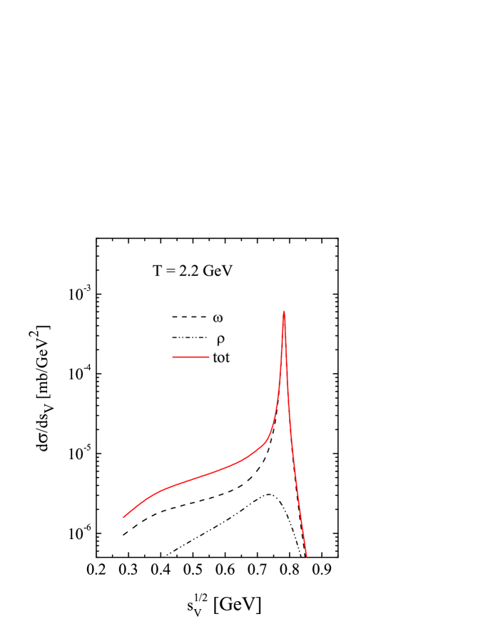
Figure 6: The same as in Fig. 5 but in a log scale. Left to the $\omega$ peak the contribution of the $\rho$ meson manifests itself as interference effect.

Results of calculations of the mass distribution $d\sigma/ds_{V}$ are presented in Figs. 5 and 6 in linear and log scales, respectively. We have chosen as kinetic beam energy $T_{beam}=2.2\,GeV$, similar to the HADES proposal HADES . The dashed line is the contribution from Dalitz decay of $\omega$ mesons $\omega\to\pi^{0}e^{+}e^{-}$, the dot-dashed line is the corresponding $\rho$ meson contribution, and the solid curve is the total cross section, including interference effects as well. It can be seen that in the very vicinity of the $\omega$ pole the contribution from $\rho$ mesons is fairly small. This is an understandable result, since the branching ratio for the Dalitz decay of $\rho$ meson is much smaller than that for the $\omega$ meson dataGroup . However, as seen from Fig. 6, outside the $\omega$ pole mass the interference effects are rather significant. Note that in the direct di-electron bremsstrahlung (two-body channel decay of vector mesons) the contribution of $\rho$ can be competitive with that of $\omega$ ourNuclPhys .

The obtained results in Figs. 5 and 6 persuade us that for the invariant mass of the $\pi e^{+}e^{-}$ subsystem close to the $\omega$ pole mass, the contribution from $\rho$ can be disregarded. This also implies that in the double differential cross section there is a suitable interval in vector meson mass $s_{V}$ in which the contribution from $\rho$ can be neglected.

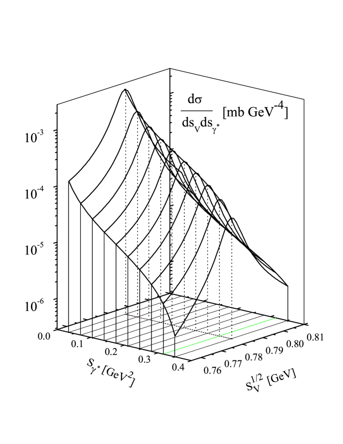
Figure 7: The double differential cross section $d\sigma/ds_{V}ds_{\gamma^{*}}$ in the vicinity of the $\omega$ pole mass $s_{\omega}^{1/2}=0.782GeV$ as a function of the di-electron invariant mass squared $s_{\gamma^{*}}$. The interval for the $\omega$ mass has been chosen with respect to the envisaged HADES resolution $\sim 3.5\%$ HADES .

In Fig. 7, results of calculations of the double differential cross section $d\sigma/ds_{V}ds_{\gamma^{*}}$ are presented as a function of the invariant mass squared of the di-electron, $s_{\gamma^{*}}$, in a narrow bin covering the $\omega$ meson pole, i.e. at mass $s_{V}\sim M_{\omega}^{2}$. It can be seen that in the whole kinematical range of the di-electron invariant mass the double differential cross section $d\sigma/ds_{V}ds_{\gamma^{*}}$ displays a narrow pronounced peak, which is governed by contributions from Dalitz decays of $\omega$ mesons. This means that by selecting events with invariant masses $s_{V}$ of the $e^{+}e^{-}\pi$ system in this interval and varying the invariant mass $s_{\gamma^{*}}$ of di-electrons, one can experimentally study the process (1) in $pp$ collisions. Let us recall in this context the studies friman1 ; rho_omega_interference , where for the exclusive reaction $\pi N\to Ne^{+}e^{-}$ the quantum interference of intermediate $\rho$ and $\omega$ mesons have been analyzed. In certain kinematical regions this interference is fairly severe and may hamper a clear distingtion of $\rho\to e^{+}e^{-}$ and $\omega\to e^{+}e^{-}$ contributions. In this respect, our calculations support a good prospect to isolate the $\omega\to\pi e^{+}e^{-}$ subreaction vs. the $\rho\to\pi e^{+}e^{-}$ part in the exclusive reaction $pp\to pp\pi^{0}e^{+}e^{-}$. For a further discussion of interference effects see below.

Let us now focus on the part of the diagrams describing the Dalitz decay of the produced vector mesons in the vicinity of the invariant mass $s_{V}=s_{\omega}$. If the contribution from only one vector meson (e.g., the $\omega$ meson) is taken into account then, as seen from eqs. (19) and (18), the cross section can be presented in the factorized form

$$\frac{d^{2}\sigma}{ds_{\gamma^{*}}ds_{V}}=\frac{\sqrt{s_{V}}/\pi}{\left(s_{V}-M_{V}^{2}\right)^{2}}\,\int d^{5}\sigma^{tot}\left(NN\to NNV\right)\,\frac{d\Gamma(V\to\pi^{0}e^{+}e^{-})}{ds_{V}},$$ (21)

where

$$d^{5}\sigma^{tot}\left(NN\to NNV\right)\,=\frac{1}{2\sqrt{\lambda(s_{0},m^{2},m^{2})}}\frac{1}{(2\pi)^{5}}\frac{1}{4}\sum\limits_{\begin{minipage}{15.6491pt} \small\footnotesize nucl.\\ spins \end{minipage}}\,\sum_{\lambda_{V}}|(J\xi_{\lambda_{V}})|^{2}d^{5}\tau(s_{12},P_{V},P_{1}^{\prime},P_{2}^{\prime})$$ (22)

is exactly the total cross section of real vector meson production in $NN$ reactions ourOmega ; ourNuclPhys . In eq. (22) we formally introduced a polarization vector $\xi_{\lambda_{V}}$ which corresponds to a real vector meson $V$ with mass $s_{V}$, $\sum_{\lambda_{V}}\xi_{\lambda_{V}}^{\alpha}\xi_{\lambda_{V}}^{+\beta}=-g^{\alpha\beta}+\frac{P_{V}^{\alpha}P_{V}^{\beta}}{P_{V}^{2}}$. Note that eqs. (21) and (22) can be easily generalized for contributions from few mesons: in such a case, the cross section will consist on a sum of two-step like cross sections (21), corresponding to each meson, and interference terms. In the mentioned kinematical bin our cross section coincides with the one obtained within a two-step mechanism with one isolated meson. However, outside this kinematical region this is not longer the case, since, apart from interference effects, even the cross section (22) is not anymore an experimentally well defined quantity, but rather describes the production of a (deeply) virtual vector meson $V$ (see discussion in ourNuclPhys ).

From (5), (21) and (22) it can be seen that the dependence upon the kinematical variables of the subprocesses $NN\to NNV$ and $\omega\to\pi^{0}e^{+}e^{-}$ can be, in principle, separated in a model independent way by performing measurements of the double differential cross section $d^{2}\sigma/ds_{\gamma^{*}}ds_{V}$ keeping the invariant mass $s_{V}$ constant and varying the di-electron mass $s_{\gamma^{*}}$. In such a way one can extract the transition FF in the same manner as in LandPhysRep ; omegaFrmf1 ; omegaFrmf2 ; omegaFrmf3 : Define the quantity

$$\left|F(s_{\gamma^{*}})\right|^{2}=\displaystyle\frac{s_{\gamma^{*}}}{s_{min}}\frac{\lambda^{3/2}(s_{\omega},s_{min},\mu_{\pi}^{2})}{\lambda^{3/2}(s_{\omega},s_{\gamma^{*}},\mu_{\pi}^{2})}\frac{\left\langle{d^{2}\sigma}/{ds_{\gamma^{*}}ds_{V}}\right\rangle}{\left\langle{d^{2}\sigma}/{ds_{\gamma^{*}}ds_{V}}\right\rangle|_{s_{\gamma^{*}}=s_{min}}},$$ (23)

where $\langle\ldots\rangle$ denotes an average about the $\omega$ pole mass corresponding to the experimental mass resolution (say, $3.5$ % as envisaged for forthcoming measurements at HADES HADES ), and $s_{min}>4m_{e}^{2}$ is the minimum value of the di-electron mass which plays a role of a normalization point. Then, as seen from eqs. (5) and (21), in the kinematical range, where the contribution of Dalitz decays of $\rho$ mesons and interference corrections are negligible, the defined quantity (23) represents indeed the transition FF $F_{\omega\pi^{0}\gamma^{*}}$.

In Fig. 8 results of calculations of the extracted FF (23) are presented for two different choices of parametrization of the input form factors. The dashed line is the subtracted FF with a VMD parametrization for both $\rho$ and $\omega$ mesons,

$$F^{VMD}_{\omega\pi^{0}{\gamma^{*}}\,}(s_{\gamma^{*}})=-\displaystyle\frac{M_{\rho}^{2}}{s_{\gamma^{*}}-(M_{\rho}-\frac{i}{2}\Gamma_{\rho})^{2}};\qquad F^{VMD}_{\rho\,\pi^{0}{\gamma^{*}}}(s_{\gamma^{*}})=-\displaystyle\frac{M_{\omega}^{2}}{s_{\gamma^{*}}-(M_{\omega}-\frac{i}{2}\Gamma_{\omega})^{2}},$$ (24)

while the solid line is the result for a nonlocal, pole-like structure of the $\omega$ meson FF

$$F^{pole}_{\omega\,\pi^{0}\gamma^{*}}(s_{\gamma^{*}})=\left(1-\frac{s_{\gamma^{*}}}{(0.65\,{\rm GeV})^{2}}\right)^{-1}.$$ (25)

For orientation, the previous experimental data on the $\omega$ meson transition FF, extracted from the reaction $\pi^{-}p\to\omega n\to n\pi^{0}\mu^{+}\mu^{-}$ at pion beam momenta of 25 and 33 $GeV/c$ LandPhysRep ; omegaFrmf1 ; omegaFrmf2 ; omegaFrmf3 is also presented in Fig. 8. A comparison of the extracted FF’s with the corresponding inputs shows that for the considered kinematical conditions, they differ by less than $0.5\%$ which demonstrates that, if the cross section is really dominated solely by resonant processes with $\omega$ and $\rho$ decays alone, the defined ratio (23) can indeed serve as convenient formula to extract the FF’s from experimental data from $pp$ collisions with high accuracy.

However, actually for processes of $NN$ scattering with a pion and a di-lepton in the final state, other, non-Dalitz type, diagrams can contribute to the cross section. In the restricted region $M_{\pi^{0}e^{+}e^{-}}\sim M_{\omega}$ these diagrams play a role of a smooth background and, in principle, can obscure the procedure of extracting FF’s by eq. (23). To estimate the effects of the background one can globally mimic it by one Feynman diagram with production and decay of an effective heavy vector meson into the considered final state with effective (freely adjustable) constants. As seen from eq. (18) the structure of the cross section is as

$$\frac{d\sigma}{ds_{\gamma^{*}}ds_{V}}\sim-\int d\Phi(s_{\gamma^{*}},s_{V},s_{12},P_{i})J_{\mu}^{(NN\to V)}\left|\frac{M_{V}^{2}}{P_{V}^{2}-(M_{V}-\frac{i}{2}\Gamma_{V})^{2}}\right|^{2}J^{+\mu(NN\to V)},$$ (26)

where $d\Phi(s_{\gamma^{*}},s_{V},s_{12},P_{i})$ is a kinematical function proportional to the phase space volume $d^{5}\tau(s_{12},P_{V},P_{1}^{\prime},P_{2}^{\prime})$. Then it is clear that the resonance structure is governed by the propagator of the $\omega$ meson, whereas the sub-diagram $NN\to NNV$ provides a smooth dependence of the cross section up on $s_{V}$. Correspondingly, one can suppose that the background cross has the same functional dependence on kinematical variables as the sub-diagram $NN\to NNV$, i.e., it is the same as $J_{\mu}^{(NN\to V)}(\omega)J^{+\mu(NN\to V)}(\omega)$ with a non-resonant (constant) propagator. As an easily trackable procedure we put the mass of the effective particle $M_{bkgr}\gg M_{\omega}$ and adopt the background cross section in the form

$$\left(\frac{d\sigma}{ds_{\gamma^{*}}ds_{V}}\right)^{(bkgr)}\sim-\int\tilde{\Phi}(s_{\gamma^{*}},s_{V},s_{12},P_{i})J_{\mu}^{(bkgr)}J^{+\mu(bkgr)}\,d^{5}\tau,$$ (27)

where $J_{\mu}^{(bkgr)}\sim\pm J_{\mu}^{(NN\to NN\omega)}$, and the function $\tilde{\Phi}(s_{\gamma^{*}},s_{V},s_{12},P_{i})$ is chosen such that the contribution of the background near the $\omega$ pole is $\sim 10\%$. This order of magnitude can be estimated from available experimental data LandPhysRep . Note that the current $J_{\mu}^{(bkgr)}$, likewise the $\omega$ and $\rho$ currents, must be transversal, i.e., $J_{\mu}^{(bkgr)}P_{V}^{\mu}=0$, which implies that this quantity necessarily depends on kinematical variables, say $J_{\mu}^{(bkgr)}=J_{\mu}^{(bkgr)}(s_{\gamma^{*}},s_{V},s_{12},P_{i})$. This means that this current can not be parameterized in an arbitrary form ; at least the condition $J_{\mu}^{(bkgr)}(s_{\gamma^{*}},s_{V},s_{12},P_{i})\ P_{V}^{\mu}=0$ must be fulfilled.

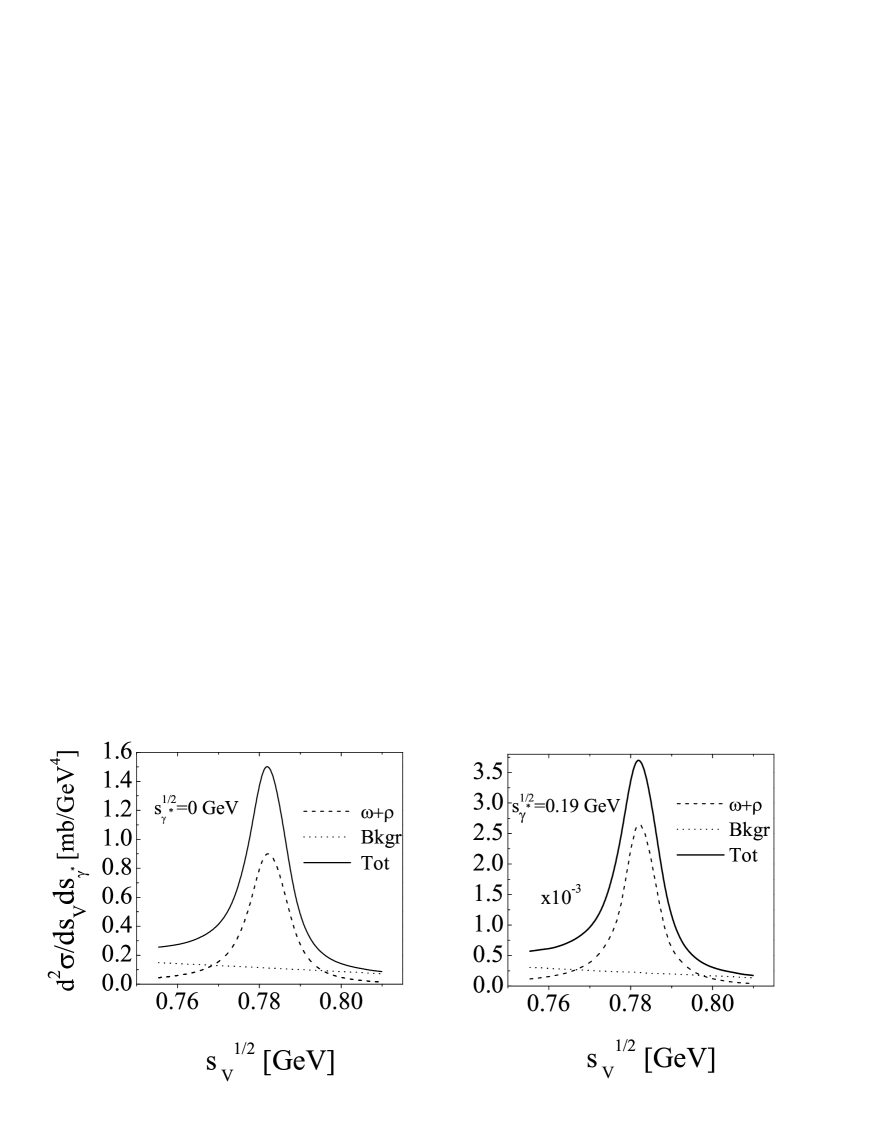
Figure 9: The double differential cross section $d\sigma/ds_{V}ds_{\gamma^{*}}$ as a function of $s_{V}^{1/2}$ in the vicinity of the $\omega$ pole for $T_{beam}=2.2\,GeV$ with background contribution taken into account. The relative sign between the resonant and background amplitudes is chosen positively resulting in a constructive interference. The dashed line corresponds to the resonant contributions of diagrams with $\omega$ and $\rho$ Dalitz decays (cf. Fig. 7), the dotted line corresponds to the background contribution alone, and the solid line is the resulting total cross section. The employed transition form factor is for the VMD model eq. (24). Left (right) panel is for $\sqrt{s_{\gamma*}}=0$ (0.19) GeV.

In Figs. 9 and 10 results of calculations of the cross section (18) with including the background (27) are presented. In Fig. 9 the relative sign of the background current is chosen positive (the interference is almost everywhere destructive), whereas in Fig. 10 the sign is negative (the interference is mainly constructive). The background (27) provides a smooth contribution to the resonant cross section; at $\omega$ peak it is about $10\%$, as dialed. However, the interference effects are rather important here and can result in corrections up to $55\%$ in the maximum. Figs. 9 and 10 also demonstrate that in case of a constructive interference the resulting cross section (solid lines) is always larger than the cross section without background contributions (dashed lines), whereas in case of a destructive interference the corresponding cross section is smaller near the peak and larger outside. These circumstances are rather important in the integrated cross sections since in the latter case the contribution of the background is partially compensated in the integral so that the FF’s extracted via eq. (23) can be quite different in the two cases. This situation is illustrated in Fig. 11, where the input FF and the extracted FF are compared. One can conclude that a constructive interference of the background may cause some uncertainty in the procedure of the experimental determination of the $\omega$ transition FF’s.

V Summary

In summary, we have analyzed the di-electron production from Dalitz decays of light vector mesons produced in $pp$ collisions at intermediate energies. The corresponding cross section has been calculated within an effective meson-nucleon approach with parameters adjusted to describe the free vector meson production ourPhi ; ourOmega in nucleon-nucleon reactions near the threshold. A possible smooth background contribution to the process has been evaluated as well. Particular attention is paid to the problem of whether it is possible to determine in such reactions the vector meson transition form factors. We argue that by studying the invariant mass distribution of the final $\pi e^{+}e^{-}$ subsystem as a function of the di-electron mass in a narrow kinematical interval near the $\omega$ meson mass one can directly measure the $\omega$ meson transition form factor $F_{\omega\pi^{0}\gamma^{*}}$ in, e.g., $pp$ collisions. Such experiments are envisaged at HADES and our results may serve as predictions for these forthcoming experiments. The uncertainties of a procedure to extract $F_{\omega\pi^{0}\gamma^{*}}$ depend upon the scale of the background processes and are expected to be small if the interference is destructive. Experimental information on form factors is useful for testing QCD predictions of hadronic quantities in the non-perturbative domain.

Appendix A Integration over decay vertices

The decay part $\left(\epsilon_{\mu\nu\beta\beta^{\prime}}P_{\gamma^{*}}^{\mu}P_{V}^{\beta^{\prime}}j_{\pm}^{\nu}\right)$ in eq. (15) can be written in the form of a current-current interaction, ${\cal J}_{(\beta)\nu}(V\to\pi^{0}\gamma\,)j_{\pm}^{\nu}$, where $j_{\pm}^{\nu}$ is the electromagnetic current of the di-electron, and the decay current is ${\cal J}_{(\beta)\nu}\sim\epsilon_{\mu\nu\beta\beta^{\prime}}P_{\gamma^{*}}^{\mu}P_{V}^{\beta^{\prime}}$. In the square of the amplitude these currents form the corresponding electromagnetic ($l^{\nu\nu\prime}$) and decay (${\cal T}_{(\beta\beta\prime)\nu\nu\prime}$) tensors, respectively. Obviously, both currents, $j_{\pm}^{\nu}$ and ${\cal J}_{(\beta)\nu}$, and consequently, both tensors are conserved:

$$P_{\gamma}^{\nu}l_{\nu\nu\prime}=P_{\gamma}^{\nu\prime}l_{\nu\nu\prime}=0;\qquad P_{V}^{\nu}{\cal T}_{(\beta\beta\prime)\nu\nu\prime}=P_{V}^{\nu\prime}{\cal T}_{(\beta\beta\prime)\nu\nu\prime}=0.$$ (28)

Consider now the integral over the di-electron phase volume. The electromagnetic tensor (16) depends only on the momenta of the virtual photon and di electron, so that the Lorentz structure, after integration over $R_{2}(\gamma\to e^{+}e^{-})$, will be governed by only two terms: one proportional to the metric tensor $g^{\nu\nu\prime}$ and another one proportional to $P_{\gamma^{*}}^{\nu}P_{\gamma^{*}}^{\nu\prime}$:

$$\int l^{\nu\nu\prime}(k_{1},k_{2},P_{\gamma^{*}})R_{2}(\gamma\to e^{+}e^{-})=a_{1}g^{\nu\nu\prime}+a_{2}P_{\gamma^{*}}^{\nu}P_{\gamma^{*}}^{\nu\prime}.$$ (29)

Equation (28) implies that $a_{1}=-a_{2}s_{\gamma^{*}}$. Multiplying (29) by $g_{\nu\nu\prime}$ one gets

$$a_{2}=-\frac{1}{3}\int[(k_{1}P_{\gamma^{*}})-s_{\gamma^{*}}]d\Omega^{*}_{\bf k}=\frac{2\pi}{3},$$ (30)

$$\int l^{\nu\nu\prime}(k_{1},k_{2},P_{\gamma^{*}})R_{2}(\gamma\to e^{+}e^{-})=\frac{2\pi}{3}s_{\gamma^{*}}\left(-g^{\nu\nu\prime}+\displaystyle\frac{P_{\gamma^{*}}^{\nu}P_{\gamma^{*}}^{\nu\prime}}{s_{\gamma^{*}}}\right).$$ (31)

Analogously, one has for the decay tensor ${\cal T}_{(\beta\beta\prime)\nu\nu\prime}$

$$\int\epsilon_{\mu\nu\alpha\beta}\epsilon_{\mu\prime\nu\alpha\prime\beta\prime}P_{\gamma^{*}}^{\mu}P_{\gamma^{*}}^{\mu\prime}P_{V}^{\alpha}P_{V}^{\alpha\prime}R_{2}(P_{V}\to k_{\pi}+P_{\gamma^{*}})=a_{1}g^{\beta\beta\prime}+a_{2}P_{V}^{\beta}P_{V}^{\beta\prime}$$ (32)

with $a_{1}=-a_{2}s_{V}$ and $a_{1}=\displaystyle\frac{\pi}{12s_{V}}\lambda^{3/2}(s_{V},\mu_{\pi}^{2},s_{\gamma^{*}})$ and

$$\int\epsilon_{\mu\nu\alpha\beta}\epsilon_{\mu\prime\nu\alpha\prime\beta\prime}P_{\gamma^{*}}^{\mu}P_{\gamma^{*}}^{\mu\prime}P_{V}^{\alpha}P_{V}^{\alpha\prime}R_{2}(P_{V}\to k_{\pi}+P_{\gamma^{*}})=\displaystyle\frac{\pi}{12s_{V}}\lambda^{3/2}(s_{V},\mu_{\pi}^{2},s_{\gamma^{*}})\left(-g^{\beta\beta\prime}+\displaystyle\frac{P_{V}^{\beta}P_{V}^{\beta\prime}}{s_{V}}\right).$$ (33)

Figure 3: Illustration of the choice of the independent variables for the process $NN\to NN+\pi+e^{+}e^{-}$ within the duplication kinematics bykling . The invariant mass squared of two final nucleons is $s_{12}$, while the invariant mass of the subsystem $\pi e^{+}e^{-}$ is $s_{V}$. The diagram depicted in left part of Fig. 1 enters here as a subprocess.

Figure 5: Differential cross section $d\sigma/ds_{V}$ for the reaction $pp\to pp+\pi+e^{+}e^{-}$ for the kinetic beam energy $T_{beam}=2.2\ GeV$. $s_{V}^{1/2}$ is the invariant mass of the subsystem $\pi e^{+}e^{-}$. Dashed and dot-dashed lines are contributions from decay of $\omega$ and $\rho$ mesons, respectively, while the dotted line is the total distribution with interference effects. The transition form factors, entering as input into the calculations, have been computed within the VMD Model (see Fig. 2).

Figure 8: The ratio (23) calculated at $T_{beam}=2.2\,GeV$ with two different transition form factors: the dashed line corresponds to the VMD model (24), while the solid line is for the dipole formula (25). The averaging in (23) has been performed in the $\pm 3.5\%$ vicinity of the $\omega$ pole mass. Experimental data are from ref. LandPhysRep .

Figure 10: The same as in Fig. 9 but with a destructive interference of resonant and background contributions.

Figure 11: The extracted FF (solid curves) by using the ratio (23) calculated at $T_{beam}=2.2\,GeV$ with inclusion of the background contribution. Dashed lines correspond to the input FF taken from the VMD model (24). The averaging has been performed in the $\pm 3.5$ % vicinity of the $\omega$ pole mass. Panels a) and b) correspond to destructive and constructive interference effects, respectively.

References

- (1) R. Rapp, J. Wambach, Adv. Nucl. Phys. 25 (2000) 1.
- (2) D. Trnka et al. (CB-TAPS Collaboration), Phys. Rev. Lett. 94 (2005) 192302.
- (3) R. Thomas, S. Zschocke, B. Kämpfer, Phys. Rev. Lett. 95 (2005) 232301.
- (4) K. Gallmeister, B. Kämpfer, O.P. Pavlenko, Phys. Rev. C 62 (2000) 057901; Phys. Lett. B 473 (2000) 20.
- (5) L.P. Kaptari, B, Kämpfer, Eur. Phys. J. A 23 (2005) 291.
- (6) L.P. Kaptari, B, Kämpfer, Eur. Phys. J. A 14 (2002) 211.
- (7) K. Nakayama, J. Haidenbauer, J. Speth, Phys. Rev. C 63 (2000) 015201.
- (8) A. Sibirtsev, J. Haidenbauer, U.-G. Meißner, nucl-th/0512055.
-
(9)
S. Okubo, Phys. Lett. 5 (1963) 165;
G. Zweig, CERN Report 8419/TH 412 (1964);
I. Iizuka, Prog. Theor. Phys. Suppl. 37/38 (1966) 21. -
(10)
A.V. Radyushkin, Phys. Rev. D 56 (1997) 5524;
M. Guidal, M.V. Polyakov, A.V. Radyushkin, M. Vanderhaeghen, Phys. Rev. D 72 (2005) 054013;
M. Diehl, Phys. Rep. 388 (2003) 41. -
(11)
V.M. Braun, A. Lenz, G. Peters, A.V. Radyushkin, hep-ph/0510237;
V.M. Braun, A. Lenz, N. Mahne, E. Stein, Phys. Rev. D 65 (2002) 07411. - (12) V.A. Novikov, M.A. Shifman, A.I. Vainshtein, M.B. Voloshin, V.I. Zakharov, Nucl. Phys. B 237 (1984) 525.
- (13) N. Isgur, C.H. Llewellyn-Smith, Nucl. Phys. B 317 (1989) 526.
-
(14)
S. Capstick, N. Isgur, Phys. Rev. D 34 (1986) 2809;
S. Godfrey, N. Isgur, Phys. Rev. D 32 (1985) 189;
K.G. Wilson, T.S. Walhout, A. Harindranath, W.-M. Zhang, R.J. Perry, Phys. Rev. D 49 (1994) 6720. -
(15)
P. Maris, P.C. Tandy, Phys. Rev. C 65 (2002) 045211;
D. Jarecke, P. Maris, P.C. Tandy, Phys. Rev. C 67 (2003) 035202. - (16) A.V. Anisovich, V.V. Anisovich, V.N. Markov, M.A. Matveev, A.V. Sarantsev, Phys. Atom. Nucl. 67 (2004) 773.
- (17) J.P.B.C. de Melo, T. Frederico, Phys. Rev. C 55 (1997) 2043; B.D. Keister, Phys. Rev. D 49 (1994) 1500.
- (18) F. Cardarelli, I. Grach, I. Narodetskii, G. Salme, S. Simula, Phys. Lett. B 359 (1995) 1.
-
(19)
V.V. Anisovich, L.G. Dakhno, M.A. Matveev, V.A. Nikonov, A.V. Sarantsev, hep-ph/0511109;
A.V. Anisovich, V.V. Anisovich, V.N. Markov, M.A. Matveev, V.A. Nikonov, A.V. Sarantsev, J. Phys. G 31 (2005) 1537. -
(20)
A.V. Anisovich, V.V. Anisovich, V.A. Nikonov, Eur. Phys. J. A 12 (2001) 103;
A.V. Anisovich, V.V. Anisovich, V.A. Nikonov, hep-ph/0305216. - (21) G. Köpp, Phys. Rev. D 10 (1974) 932.
-
(22)
A. Faessler, C. Fuchs, M. Krivoruchenko, Phys. Rev. C 61 (2000) 035206;
H.C. Dönges, M. Schäfer, U. Mosel, Phys. Rev. C 51 (1995) 950. - (23) H.B.H. O’Connel, B.C. Pearce, A.W. Thomas, A.G. Williams, Prog. Nucl. Part.
-
(24)
U.-G. Meißner, Phys. Rep. 161 (1988) 213;
N.M. Kroll, T.D. Lee, B. Zumino, Phys. Rev. 157 (1967) 1376. - (25) F. Klingl, N. Kaiser, W. Weise, Z. Phys. A 356 (1996) 193.
- (26) Ö. Kaymakcalan, S. Rajeev, J. Schechter, Phys. Rev. D 30 (1984) 594.
-
(27)
P. Salabura et al. (HADES Collaboration), Acta Phys. Pol. B 35 (2004) 1119;
R. Holzmann et al. (HADES Collaboration), Prog. Part. Nucl. Phys. 53 (2004) 49. - (28) L.G. Landsberg, Phys. Rep. 128 (1985) 301.
- (29) R.I. Dzhelyadin, S.V. Golovkin, M.V. Gritsuk, D.B. Kakauridze et al., Phys. Lett. B 84 (1979) 143; Phys. Lett. B 88 (1979) 379.
- (30) R.I. Dzhelyadin, S.V. Golovkin, A.S. Konstantinov, V.P. Kubarovski et al., Phys. Lett. B 102 (1981) 296.
- (31) V.A. Viktorov, S.V. Golovkin, R.I. Dzhelyadin, V.P. Kubarovski et al., Yad. Fiz. 32 (1980) 998, 1002, 1005; Phys. Lett. 94B (1980) 548.
- (32) S. Eidelman et al. (Particle Data Group), Phys. Lett. B 592 (2004).
- (33) M.F.M. Lutz, B. Friman, M. Soyeur, Nucl. Phys. A 713 (2003) 97.
- (34) B. Friman, M. Soyeur, Nucl. Phys. A 600 (1996) 477.
- (35) E. Byckling, K. Kajantie, ”Particle Kinematics”, John Wiley & Sons 1973.
- (36) K. Nakayama, J.W. Durso, J. Haidenbauer, C. Hanhart, J. Speth, Phys. Rev. C 60 (1999) 055209.
- (37) L.P. Kaptari, B. Kämpfer, Nucl. Phys. A 764 (2006) 338.
- (38) A.I. Titov, B. Kämpfer, B.L. Reznik, Eur. Phys. J. A 7 (2000) 543; Phys. Rev. C 65 (2002) 065202.
- (39) J. Gillespie, ” Final State Interactions”, Holden-Day Advanced Physics Monographs, 1964.
-
(40)
M. Büscher et al., ”Study of and meson
production in the reaction at ANKE”,
experiment proposal #75/ANKE, cf.
http://ikpd15.ikp.kfa-juelich.de:8085/doc/Proposals.html;
www.fz-juelich.de/ikp/anke/doc/Proposals.shtml - (41) A.I. Titov, B. Kämpfer, Eur. Phys. J. A 12 (2001) 217.