Nuclear symmetry energy effects on neutron stars properties

Abstract

We construct a class of nuclear equations of state based on a schematic potential model, that originates from the work of Prakash et. al. [1], which reproduce the results of most microscopic calculations. The equations of state are used as input for solving the Tolman-Oppenheimer-Volkov equations for corresponding neutron stars. The potential part contribution of the symmetry energy to the total energy is parameterized in a generalized form both for low and high values of the baryon density. Special attention is devoted to the construction of the symmetry energy in order to reproduce the results of most microscopic calculations of dense nuclear matter. The obtained nuclear equations of state are applied for the systematic study of the global properties of a neutron star (masses, radii and composition). The calculated masses and radii of the neutron stars are plotted as a function of the potential part parameters of the symmetry energy. A linear relation between these parameters, the radius and the maximum mass of the neutron star is obtained. In addition, a linear relation between the radius and the derivative of the symmetry energy near the saturation density is found. We also address on the problem of the existence of correlation between the pressure near the saturation density and the radius.

Keywords: nuclear symmetry energy; nuclear equation of state; neutron stars.
PACS : 26.60.+c; 97.60.Jd; 21.65.+f; 21.60.-n

1 Introduction

Neutron stars (NS) are some of the densest manifestations of massive objects in the universe which provide very rich information for testing theories of dense matter physics and also provide a connection among nuclear physics, particle physics, statistical physics and astrophysics [2, 3, 4, 5, 6, 7, 8, 9, 10, 11]. The global aspects of neutron stars, such as the masses, radii and composition are determined by solving the so-called Tolman-Oppenheimer-Volkov (TOV) equations [12, 13]. However there are large variations in predicted radii and maximum masses because of the uncertainties in the nuclear equation of state (EOS) near and mainly above the saturation density $n_{s}$ [8, 14, 15, 16, 17, 18, 19, 20, 21, 22, 23, 24, 25, 26, 27, 28, 29, 30, 31, 32, 33, 34, 35, 36]. The total energy of neutron rich matter (the case of a neutron star) can be written as a sum of two parts. The first one is the contribution of the symmetric nuclear matter (which is well known) and the second is the symmetry energy (SE) which still is uncertain although several constraints exist from ground state masses (binding energies) and giant dipole resonances of laboratory nuclei. A consequence of this uncertainty is that different models predict up to a factor of 6, variations in the pressure of neutron star matter near $n_{s}$, even though the pressure of symmetric matter is better known, being nearly zero at the same density. This pressure variation accounts for the nearly 50% variation in the predictions of neutron star radii [2, 37].

In general, the value of the SE at nuclear saturation density and mainly the density dependence of the SE are both difficult to be determined in the laboratory. The motivation of the present work is to propose a new parameterization for the potential part of the symmetry energy $E_{sym}(n)$ in order to be able to reproduce the results of a variety of microscopic models both in low and high values of the baryon density. Especially the trend of the symmetry energy just above the equilibrium density $n_{s}$ is a critical factor in determining the neutron star radius.

In order to calculate the global properties of neutron stars (mass, radius ets.) the hydrostatic equilibrium equations of Tolman, Oppenheimer and Volkov have to be solved once the equation of state is specified. However, the composition of a neutron star still remains uncertain and the construction of the EOS, which is based on the ingredients of the NS’s and the kind of interactions which characterize them, is subjected to several assumptions. In any case the calculated EOS has to satisfy the following requirements [29]: i) It must display the correct saturation point for symmetric nuclear matter (SNM); ii) it must give a SE compatible with nuclear phenomenology especially at high densities; iii) for SNM the incompressibility at saturation must be compatible with the values extracted from phenomenology; iv) both for neutron matter and SNM the speed of sound must not exceed the speed of light (causality condition), at least up to the relevant densities.

In the present work we consider that the neutron star core is composed only by an uncharged mixture of neurons, protons and electrons in equilibrium with respect to the weak interaction ($\beta$-stable matter). However in general, in the range of densities $n\geq n_{s}$, the hadronic phase of superdense matter with a rich spectrum of particles (hyperons, baryonic resonances, $\pi^{-}$ and $K^{-}$ mesons, and a small portion of leptons) is realized. The model which is used for the construction of the EOS is a generalization of a schematic potential model based on a previous work of Prakash et al. [1]. The model reproduces the results of most microscopic calculations of dense matter [25]. It is worthwhile to notice that there many ways to determine the equation of state through the many-body approach of interacting hadrons. Some of the most recent ones are based on variational methods [38, 39, 40] and some are based on microscopic calculations [41]. In order to face the problem that stems from the uncertain behavior of the SE at high densities we perform a suitable parameterization both in low and high densities. In the previous work of Prakash et al [1, 9] the parameterization of the potential term of the SE is achieved by the introduction of three different choices of the potential contribution to the SE. To advance, in the present work, we suggest a more generalized parameterization of the potential term of the SE which is more flexible and efficient, reproduces the predictions of most microscopic calculations of dense matter [25] and confirms the results of various empirical data.

The most striking feature of the proposed parameterization is the different form of the parameterization function $F(u)$ for densities below saturation point and for densities above this point. This is not surprising since this was already entailed in microscopic calculations. Although the behavior of the SE for densities below the saturation point still remains unknown, significant progress has been made only most recently in constraining the SE at subnormal densities and around the normal density from the isospin diffusion data in heavy-ion collisions [42, 43]. This has led to a significantly more refined constraint on neutron-skin thickness of heavy nuclei [44, 45] and the mass-radius correlation of neutron stars [33, 34, 35]. For densities above the saturation point the trend of the SE is model dependent and exhibits completely different behavior.

The above characteristic of the SE is well reflected in our proposed models. In view of the previous comment, the proposed parameterization of the potential term of the SE has the advantage to be able to reproduce microscopic calculations in cases where the SE, at low densities, increases along with the density and then begins to fall although the density continues to increase. This is a well known characteristic of a class of Skyrme interactions [16, 17, 18] and of Gogny Hartree-Fock calculations [33, 34, 35]. Special effort has been devoted to find analytical relations between the radius $R$ and the pressure $P$ which correspond to a special density $n$ for a fixed value of the mass $M$ of the neutron star. So an accurate determination of a neutron star radius will permit evaluation of the pressure of neutron star matter. All the above will provide a direct determination of the density dependence of the nuclear SE at these densities [37, 46].

Finally, we also address on the problem of neutron star cooling [47, 48]. It is well known that the direct Urca process can occur in neutron stars if the proton concentration exceeds some critical value in the range of 11-15 %. The proton concentration can be determined by the trend of the SE especially just above the equilibrium density. So, the detailed knowledge of the SE behavior is crucial for the existence of the direct Urca process.

The plan of the paper is as follows. In section $2$ the proposed model and the relatives formulas are discussed and analyzed. Results are reported and discussed in section $3$, while the summary of the work is given in section $4$.

2 The model

In general, the energy per baryon of neutron-rich matter may be written as

$$\frac{E(n,x)}{A}=\frac{E(n,\frac{1}{2})}{A}+(1-2x)^{2}E_{sym}^{(2)}(n)+(1-2x)^{4}E_{sym}^{(4)}(n)+\cdots\ ,$$ (1)

To a good approximation, it is sufficient to retain in the above expansion only the quadratic term. Thus, the above equation takes the form

$$\frac{E(n,x)}{A}=\frac{E(n,\frac{1}{2})}{A}+(1-2x)^{2}E_{sym}^{(2)}(n)\ ,$$ (2)

where $n$ is the baryon density ($n=n_{n}+n_{p}$) and $x$ is the proton fraction ($x=n_{p}/n$). The symmetry energy $E_{sym}(n)=E_{sym}^{(2)}(n)$ can be expressed in terms of the difference of the energy per baryon between neutron ($x=0$) and symmetry ($x=1/2$) matter

$$E_{sym}(n)=\frac{E(n,0)}{A}-\frac{E(n,\frac{1}{2})}{A}\ .$$ (3)

In the present work we consider a schematic equation for symmetric nuclear matter energy (energy per baryon $E/A$ or equivalently the energy density per nuclear density $\epsilon/n$) which is given by the expression [1]

$$\frac{E(n,1/2)}{A}=\frac{\epsilon_{sym}}{n}=m_{N}c^{2}+\frac{3}{5}E_{F}^{0}u^{2/3}+V(u),\qquad u=n/n_{s}$$ (4)

where $E_{F}^{0}=(\hbar k_{F}^{0})^{2}/2m_{N}$ is the Fermi energy per baryon in equilibrium state and $n_{s}$ is the saturation density.

The density dependent potential energy per nucleon $V(u)$ of the symmetric nuclear matter is parameterized, based on the previous work of Prakash et. al. [1, 9] as follows

$$V(u)=\frac{1}{2}Au+\frac{Bu^{\sigma}}{1+B^{\prime}u^{\sigma-1}}+3\sum_{i=1,2}C_{i}\left(\frac{\Lambda_{i}}{p_{F}^{0}}\right)^{3}\left(\frac{p_{F}}{\Lambda_{i}}-\arctan\frac{p_{F}}{\Lambda_{i}}\right),$$ (5)

where $p_{F}$ is the Fermi momentum, related to $p_{F}^{0}$ by $p_{F}=p_{F}^{0}u^{1/3}$. The parameters $\Lambda_{1}$ and $\Lambda_{2}$ parameterize the finite forces between nucleons. The values used here are $\Lambda_{1}=1.5p_{F}^{0}$ and $\Lambda_{2}=3p_{F}^{0}$. The parameters $A$, $B$, $B^{\prime}$, $\sigma$, $C_{1}$ and $C_{2}$ are determined with the constraints provided by the properties of nuclear matter saturation. In the present work the values of the above parameters are determined in order that $E(n=n_{s})/A-m_{N}c^{2}=-16$ MeV, $n_{s}=0.16$ fm^-3 and $K_{0}=240$ MeV. In general the parameter values for three possible values of the compression modulus $K_{0}$ $\left(K_{0}=9n_{0}^{2}\frac{d^{2}(E/A)}{dn^{2}}|_{n_{0}}\right)$ are displayed in table I, on Ref. [1].

To a very good approximation, the nuclear symmetry energy $E_{sym}$ can be parameterized as follows [6]

$$E_{sym}(u)=\left(2^{2/3}-1\right)\frac{3}{5}E_{F}^{0}\left(u^{2/3}-F(u)\right)+S_{0}F(u),$$ (6)

where $S_{0}$ is the SE at the saturation point, $S_{0}=E_{sym}(u=1)$. In general, theoretical predictions give $S_{0}=25-35$ MeV. In the present work we consider $S_{0}=30$ MeV. The function $F(u)$ parameterizes the potential contribution of the nuclear SE and has to satisfy the constraints $F(u=0)=0$ and $F(u=1)=1$. Equation (6) can be written in a more instructive form by separating the kinetic and the potential contribution of the SE.

$$E_{sym}(u)\simeq\underbrace{13u^{2/3}}_{Kinetic}+\underbrace{17F(u)}_{Potential}.$$ (7)

In the previous work of Prakash et. al. [1], three representative forms that mimic the results of most microscopic models are used and have the following form

$$F(u)=u,\qquad F(u)=\frac{2u^{2}}{1+u},\qquad F(u)=\sqrt{u}.$$ (8)

In the present work we generalize the previous form of the function $F(u)$ in two ways. First, the function $F(u)$ is parameterized as follows

$$F(u)=u^{c},$$ (9)

where the parameter $c$ (hereafter called potential parameter) varies between $0.4<c<1.5$ in order to get reasonable values for the SE. It is obvious that according to the above formula the trend of the potential part is the same both in low and high values of the baryon density.

The information gained from microscopic theoretical calculations shows that this is not the general case for the potential part of the SE. On the contrary, the SE exhibits different trends in low and high densities. So, one should try to find a new formula for the function $F(u)$ which satisfies the above restrictions. In the spirit of the previous statement we propose a new parameterization of the function $F(u)$. The new function which is more flexible compared to the previous ones, reproduces the SE for most realistic calculations and has the following form

$$F(u) = \left\{\begin{array}[]{ll}u^{c_{1}}&\mbox{$u\leq 1$}\\ \\ u^{c_{2}}e^{1-u}+(u-1)(c_{1}+1-c_{2})&\mbox{$u\geq 1$}\ .\end{array}\right.$$ (13)

The function $F(u)$ satisfies the constraints $F(u\rightarrow 1^{+})=F(u\rightarrow 1^{-})$ and $F^{\prime}(u\rightarrow 1^{+})=F^{\prime}(u\rightarrow 1^{-})$. The derivative of the function, compared to equation (9), is determined by the parameters $c_{1}$ and $c_{2}$ (hereafter called potential parameters).

In order to construct the nuclear equation of state, the expression of the pressure is needed. In general, the pressure, at temperature $T=0$, is given by the expression

$$P=n^{2}\frac{d(\epsilon/n)}{dn}=n\frac{d\epsilon}{dn}-\epsilon.$$ (14)

From equations (2), (4) and (14) we found that the contribution of the baryon to the total pressure is given by the relation

$$P_{b}=\left[\frac{2}{5}E_{F}^{0}n_{s}u^{5/3}+u^{2}n_{s}\frac{dV(u)}{du}\right]+n_{s}(1-2x)^{2}u^{2}\frac{dE_{sym}(u)}{du}.$$ (15)

The leptons (electrons and muons) originating for the condition of the beta stable matter contribute also to the total energy and total pressure [6]. To be more precise the electrons and the muons which are the ingredients of the neutron star are considered as non-interacting Fermi gases. In that case their contribution to the total energy and pressure is given by

$$\epsilon_{e^{-},\mu^{-}}=\frac{m_{l}^{4}c^{5}}{8\pi^{2}\hbar^{3}}\left[(2z^{3}+z)(1+z^{2})^{1/2}-\sinh^{-1}(z)\right],$$ (16)

$$P_{e^{-},\mu^{-}}=\frac{m_{l}^{4}c^{5}}{24\pi^{2}\hbar^{3}}\left[(2z^{3}-3z)(1+z^{2})^{1/2}+3\sinh^{-1}(z)\right],$$ (17)

where $z=k_{F}/m_{l}c$. Now the total energy and pressure of charge neutral and chemically equilibrium nuclear matter is

$$\epsilon_{tot}=\epsilon_{b}+\sum_{l=e^{-},\mu^{-}}\epsilon_{l},$$ (18)

$$P_{tot}=P_{b}+\sum_{l=e^{-},\mu^{-}}P_{l}\ .$$ (19)

From equations (18) and (19) we can construct the equation of state in the form $\epsilon=\epsilon(P)$. What remains is the determination of the proton fraction $x$ in $\beta$-stable matter. In that case we have the process

$$n\longrightarrow p+e^{-}+\bar{\nu}_{e}\qquad\qquad p+e^{-}\longrightarrow n+\nu_{e}$$ (20)

that takes place simultaneously. We assume that neutrinos generated in these reactions have left the system. This implies that

$$\hat{\mu}=\mu_{n}-\mu_{p}=\mu_{e},$$ (21)

where $\mu_{n},\mu_{p}$ and $\mu_{e}$ are the chemical potential of the neutron, proton and electron respectivelly. Given the total energy density $\epsilon\equiv\epsilon(n_{n},n_{p})$, the neutron and proton chemical potential can be defined as

$$\mu_{n}=\frac{\partial\epsilon}{\partial n_{n}}|_{n_{p}},\qquad\qquad\mu_{p}=\frac{\partial\epsilon}{\partial n_{p}}|_{n_{n}}.$$ (22)

It is easy to show that after some algebra we get

$$\hat{\mu}=\mu_{n}-\mu_{p}=-\frac{\partial\epsilon/n}{\partial x}|_{n}=\frac{\partial E}{\partial x}|_{n}.$$ (23)

In $\beta$ equilibrium one has

$$\frac{\partial E}{\partial x}=\frac{\partial}{\partial x}\left(E_{b}(n,x)+E_{e}(x)\right)=0,$$ (24)

where $E_{b}(n,x)$ the energy per baryon and $E_{e}(x)$ the electron energy. The charge condition implies that $n_{e}=n_{p}=nx$ or $k_{F_{e}}=k_{F_{p}}$. Combining the relations (2) and (23) we get

$$\hat{\mu}=4(1-2x)E_{sym}(n).$$ (25)

Finally by combining equations (21) and (25) we arrive at the relation

$$4(1-2x)E_{sym}(n)=\hbar c(3\pi^{2}n_{e})^{1/3}=\hbar c(3\pi^{2}nx)^{1/3},$$ (26)

where we considered that the chemical potential of the electron is given by the relation $\mu_{e}=\sqrt{k_{F_{e}}^{2}c^{2}+m_{e}^{2}c^{4}}\approx k_{F_{e}}c$ (relativistic electrons). Equation (26) determines the equilibrium proton fraction $x(n)$ once the density dependent symmetry energy $E_{sym}(n)$ is known. After straightforward algebra we get

$$x(n)=\frac{1}{2}-\frac{1}{4}\left([2\beta(\gamma-1)]^{1/3}-[2\beta(\gamma+1)]^{1/3}\right),$$ (27)

where

$$\beta=3\pi^{2}n(\hbar c/4E_{sym}(n))^{3},\qquad\qquad\gamma=\left(1+\frac{2\beta}{27}\right)^{1/2}.$$

When the electrons energy is large enough (i.e. greater than the muon mass), it is energetically favorable for the electrons to convert to muons

$$e^{-}\longrightarrow\mu^{-}+\bar{\nu}_{\mu}+\nu_{e}.$$ (28)

However, in the present work we will not include the muon case to the total equation of state since the muon contribution does not alter significantly the gross properties of the neutron stars.

It is worthwhile to notice that the present model satisfies the relativistic causality. That means the speed of sound which was defined from the relation,

$$\left(\frac{c_{s}}{c_{l}}\right)^{2}=\frac{dP}{d\epsilon}=\frac{dP/dn}{d\epsilon/dn},$$ (29)

does not exceed the speed of light for any value of the baryon density. This is a basic treat for any realistic EOS, regardless the details of the interactions among matter constituents or the many body approach [29].

The most efficient process, which leads to a fast cooling of a neutron star, is the direct Urca process involving nucleons

$$n\longrightarrow p+e^{-}+\bar{\nu}_{e},\qquad\qquad p+e^{-}\longrightarrow n+\nu_{e}\ .$$ (30)

This process is only permitted if energy and momentum can be simultaneously conserved [47, 48]. This requires that the proton fraction must be $x>1/9\simeq 0.11$. From equation (27) it is obvious that the proton fraction $x$ is sensitive to the density dependence of the SE and as consequence to the parameterization of the potential part of $E_{sym}(n)$. So, in the present work it is worthwhile to study the relation of the proton fraction and the relative parameterization and also to check if our parameterization satisfies the constraints for the beggining of the Urca process.

In order to calculate the gross properties of a NS we assume that a NS has a spherically symmetric distribution of mass in hydrostatic equilibrium and is extremely cold ($T=0$). Effects of rotations and magnetic fields are neglected and the equilibrium configurations are obtained by solving the Tolman-Oppenheimer-Volkoff equations [12, 13]

$$\frac{dP(r)}{dr} = -\frac{Gm(r)\rho(r)}{r^{2}}\left(1+\frac{P(r)}{c^{2}\rho(r)}\right)\left(1+\frac{4\pi r^{3}P(r)}{c^{2}m(r)}\right)\left(1-\frac{2Gm(r)}{c^{2}r}\right)^{-1},$$

$$\frac{dM(r)}{dr} = 4\pi r^{2}\rho(r)=\frac{4\pi r^{2}\epsilon(r)}{c^{2}}.$$ (31)

To solve the set of equations (31) for $P(r)$ and $M(r)$ one can integrate outwards from the origin ($r=0$) to the point $r=R$ where the pressure becomes zero. This point defines R as the coordinate radius of the star. To do this, one needs an initial value of the pressure at $r=0$, called $P_{c}=P(r=0)$. The radius $R$ and the total mass of the star, $M\equiv M(R)$, depend on the value of $P_{c}$. To be able to perform the integration, one also needs to know the energy density $\epsilon(r)$ (or the density mass $\rho(r)$) in terms of the pressure $P(r)$. This relationship is the equation of state for neutron star matter and in the present work has been calculated for various cases by using our model. It should also be noted that besides the stellar radius and mass, other global attributes of a neutron star are potentially observable, including the moment of inertia and the binding energy [37, 49]. Thus, it would be of interest to study the nuclear symmetry dependence on these attributes. Such work is in progress.

3 Results and discussion

First we apply our model in a simple case where the potential part of the SE is parameterized as $F(u)=u^{c}$ and the total SE contribution can be written as follows

$$E_{sym}(u)=13u^{2/3}+17u^{c}.$$ (32)

The potential parameter $c$ varies between $0.4\leq c\leq 1.5$ which gives reliable values of the SE. The total pressure of the cold beta-stable nucleonic matter is given by

$$P(n,x)=n^{2}\left[\frac{E^{\prime}(n,\frac{1}{2})}{A}+E_{sym}^{\prime}(n)(1-2x)^{2}\right]+P_{e^{-}}(n),$$ (33)

where $E_{sym}^{\prime}(n)$ takes the form

$$E_{sym}^{\prime}(n)\equiv\frac{dE_{sym}(n)}{dn}=\frac{1}{n_{s}}\left[\frac{26}{3}u^{-1/3}+17cu^{c-1}\right].$$ (34)

We are interested for the total pressure at the saturation density $n_{s}$. Considering that the electron pressure $P_{e^{-}}(n)$ is [37]

$$P_{e^{-}}(n)\cong nx(1-2x)E_{sym}(n)$$ (35)

then the total pressure at $n_{s}$ is given by the expression [37]

$$P_{s}(n_{s},x_{s})=n_{s}(1-2x_{s})\left[n_{s}E_{sym}^{\prime}(n_{s})(1-2x_{s})+E_{sym}(n_{s})x_{s}\right],$$ (36)

where $E_{sym}^{\prime}(n_{s})=\left[\frac{dE_{sym}(n)}{dn}\right]_{n=n_{s}}$ and the equilibrium proton fraction at $n_{s}$ is given

$$x_{s}\simeq(3\pi^{2}n_{s})^{-1}(4E_{sym}(n_{s})/\hbar c)^{3}\simeq 0.04.$$ (37)

For small values of $x_{s}$ we find that

$$P_{s}(n_{s},x_{s})\simeq n_{s}^{2}E_{sym}^{\prime}(n_{s}).$$ (38)

From the former expression it is obvious that the pressure is mostly sensitive to the density dependence of the SE at the saturation point $n_{s}$. Using our model from equation (34) we get

$$E_{sym}^{\prime}(n_{s})\simeq\frac{1}{n_{s}}\left(\frac{26}{3}+17c\right).$$ (39)

From equations (38) and (39) it is concluded that the relation between the pressure $P_{s}$ and the potential parameter $c$ is

$$P_{s}(n_{s},x_{s})\simeq n_{s}\left(\frac{26}{3}+17c\right).$$ (40)

In order to calculate the global properties of the neutron star, radius and mass we solved numerically the TOV equations (31) with the given equations of state constructed with the present model. For very low densities ($n<0.08$ fm^-3) we used the equation of state taken from Feynman, Metropolis and Teller [50] and also from Baym, Bethe and Sutherland [51].

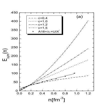
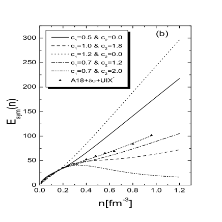
Figure 1: (a) $E_{sym}(n)$ for various values of the potential parameter $c$ of the function $F(u)$, given by the equation (9), versus the baryon density $n$. The case A18+$\delta$u+UIX^∗ from Ref. [39] is also included with the least-squares fit curve which corresponds to the value $c=0.9$ (b) $E_{sym}(n)$ for various values of the potential parameters $c_{1}$ and $c_{2}$ of the function $F(u)$, given by the equation (13), versus the baryon density $n$. The case A18+$\delta$u+UIX^∗ from Ref. [39] is also included with the least-squares fit curve which corresponds to the values $c_{1}=0.77$ and $c_{2}=1.09$.

In order to illustrate the density dependence trend of the SE proposed in our model we display in figure 1a $E_{sym}(n)$ as a function of the density $n$ for various values of the potential parameter $c$. It is obvious that the parameter $c$ affects decisively the trend of the SE, especially at high values of the density. So, it is very interesting to study how the values of the parameter $c$, and consequently the potential contribution, affect the gross properties of the NS. In the same figure, results of Ref. [39] (the case A18+$\delta$u+UIX^∗, see TABLE VI and VII of Ref. [39]) are included. It is found that the use of the phenomenological equation (7) with proper value ($c=0.9$) of function (9) reproduces the results of the above microscopic calculations.

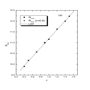
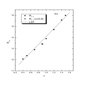
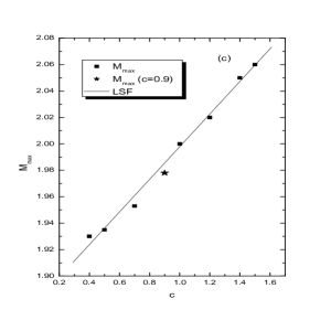
Figure 2: (a) The radius $R_{max}$ as a function of the parameter $c$. (b) The radius $R_{1.4}$ as a function of the parameter $c$. (c) The maximum mass $M_{max}$ of the neutron star as a function of the parameter c. The solid lines correspond to the least-squares fit expressions (LSF) (41), (42) and (43) respectively. In all figures the star symbol corresponds to the case $A18+\delta u+UIX^{*}$ ( $c=0.9$).

Figure 2a demonstrates the linear dependence between the radius $R_{max}$ and the parameter $c$. From our analysis it is concluded that there is a direct relation between $R_{max}$ and the parameterization of the potential part of the SE. The star symbol corresponds to the case A18+$\delta$u+UIX^∗ with $c_{1}=0.9$. The corresponding relation was derived with the least-squares fit method and has the form

$$R_{max}=9.10195+2.08304c.$$ (41)

In addition, in figure 2b we indicate the behavior of the neutron star radius $R_{1.4}$, which corresponds to a neutron star mass $M=1.4M_{\odot}$, versus the parameter $c$. The star symbol corresponds to the case A18+$\delta$u+UIX^∗ with $c_{1}=0.9$. It is obvious that there is also a linear relation between $R_{1.4}$ and $c$ which is

$$R_{1.4}=10.52114+3.56746c.$$ (42)

Figure 2c displays the correlation between the maximum mass of the neutron star $M_{max}$ and the parameter $c$. The star symbol corresponds to the case A18+$\delta$u+UIX^∗ with $c_{1}=0.9$. We found an almost linear relation between $M_{max}$ and $c$ which has the form

$$M_{max}=1.87442+0.12344c.$$ (43)

By combining equations (39) and (42) we found a linear relation between $R_{1.4}$ and $E^{\prime}_{sym}(n_{s})$ which has the form

$$R_{1.4}=8.702+0.0336E^{\prime}_{sym}(n_{s}),$$ (44)

and vice-versa

$$E^{\prime}_{sym}(n_{s})=-259.185+29.783R_{1.4}.$$ (45)

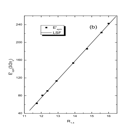
Figure 3: (a) The radius $R_{1.4}$ versus the derivative of the Symmetry Energy $E^{\prime}_{sym}(3n_{s}/2)$. (b) $E^{\prime}_{sym}(3n_{s}/2)$ versus $R_{1.4}$. The solid lines correspond to the least-squares fit (LSF) expressions (46) and (47) respectively.

In order to illustrate further the relation between the radius $R_{1.4}$ and the trend of the SE we plot in figure 3a the radius $R_{1.4}$ versus the derivative of the symmetry energy $E^{\prime}_{sym}(3n_{s}/2)$ at the baryon density $n=3n_{s}/2$. A linear relation is found, which has the form

$$R_{1.4}=10.1798+0.0242E^{\prime}_{sym}(3n_{s}/2).$$ (46)

It is concluded that there is a direct relation between the radius $R_{1.4}$ and the trend of the SE, close to the saturation point $n_{s}$. In addition in figure 3b we plot $E^{\prime}_{sym}(3n_{s}/2)$ versus $R_{1.4}$ with the linear correlation

$$E^{\prime}_{sym}(3n_{s}/2)=-420.40895+41.3066R_{1.4}.$$ (47)

To ensure the relativistic causality in the present model we display figure 4a, where the ratio of the speed of sound to speed of light $c_{s}/c_{l}$ is plotted versus the baryon density for various values of the parameter $c$. Evidently, in all cases the speed of sound does not exceed that of light even at high values of the baryon density. In addition in figure 4b we plot the proton fraction $x_{p}$ calculated from expression (27) as a function of the baryon density $n$. It is obvious that only in the cases where $c>0.5$ the proton fraction, after a specific density, exceed the critical value $x^{Urca}\simeq 0.11$ which ensures the beginning of the Urca process.

We also tried to find the correlation between the pressure $P$ (and consequently the radius R) and the SE for other values of the density $n$. In order to clarify the problem of the expected relation between the radius and the pressure we present a more simplified model of a non-relativistic equation with a polytrope type of EOS. Thus the EOS has the form [3, 37]

$$P=K\rho^{\gamma},\qquad\gamma=1+\frac{1}{\lambda}.$$ (48)

and the radius of the star is given by

$$R=\left[\frac{(\lambda+1)K}{4\pi G}\right]^{1/2}\rho_{c}^{(1-\lambda)/2\lambda}\xi_{1},$$ (49)

where $\rho_{c}$ is the central density and $\xi_{1}$ is the solution of the equation $\theta(\xi_{1})=0$, where the function $\theta(\xi)$ is the solution of the differential Lane-Emden equation

$$\frac{1}{\xi^{2}}\frac{d}{d\xi}\xi^{2}\frac{d\theta}{d\xi}=-\theta^{\lambda}.$$ (50)

Now it is obvious from equations (48) and (49) that in case $\lambda=1$ (or $\gamma=2$) where $\xi=\pi$ we have

$$\frac{R}{P^{1/2}}=\left[\frac{2G}{\pi}\right]^{1/2}\frac{1}{\rho}\ .$$ (51)

Thus, from equation (51) we concluded that in the case of a polytrope with $\gamma=2$ there is a universal relation of the ratio $R/P^{1/2}$ calculated for a specific value of the density $\rho$. However if general relativity effects are included in the above analysis the exponent $1/2$ of the pressure is found to be smaller [37].

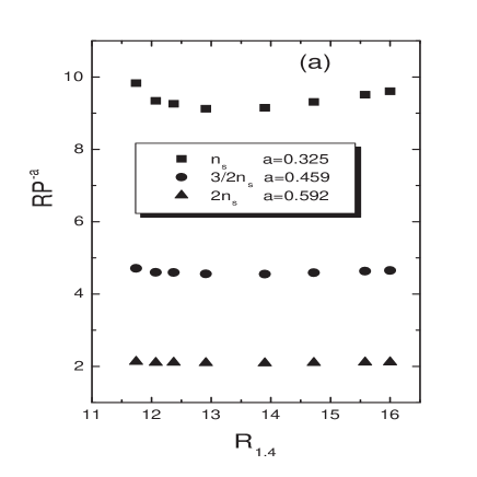
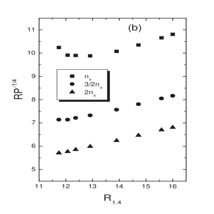
Figure 5: (a) The quantity $RP^{-a}$ as a function of the radius $R_{1.4}$ for pressure determined at $n=n_{s}$, $n=3n_{s}/2$ and $n=2n_{s}$. For each density, the least-squares fit value for the exponent $a$ is indicated. (b) The quantity $RP^{-1/4}$ as a function of the radius $R_{1.4}$ for pressure determined at $n=n_{s}$, $n=3n_{s}/2$ and $n=2n_{s}$.

Following the above statement we plot in figure 5a the quantity $R_{1.4}P^{-a}$ as a function of the radius $R_{1.4}$. One can see that there is a correlation between the radii $R_{1.4}$ and the pressure evaluated at densities $1n_{s}$, $3n_{s}/2$ and $2n_{s}$. The values of the parameters $a$ and $C(n)$ have been defined by least-squares fit of the expression $R_{1.4}=C(n)P^{a}$.

In addition, in figure 5b we plot the quantity $R_{1.4}R^{-1/4}$ as a function of the $R_{1.4}$ to compare it with the previous work of Lattimer et. al [37]. It is worthwhile to notice that the quantity $R_{1.4}R^{-1/4}$ is a mild increasing function of the radius $R_{1.4}$. This effect is more evident for densities far from the saturation( $n=3n_{s}/2,2n_{s}$). So, from our study it is concluded that there is a slight dependence of the quantity $R_{1.4}R^{-1/4}$ from the potential parameter $c$ and consequently from the trend of the SE.

We proceed now in the more complicated case where the function $F(u)$ is given by expression (13). In that case the derivative of the $E_{sym}(n)$ is given by

$$E_{sym}^{\prime}(n) = \left\{\begin{array}[]{ll}\frac{1}{n_{s}}\left[\frac{26}{3}u^{-1/3}+17c_{1}u^{c_{1}-1}\right]&\mbox{$u\leq 1$}\\ \\ \frac{1}{n_{s}}\left[\frac{26}{3}u^{-1/3}+17\left(c_{1}+1-c_{2}+e^{1-u}u^{c_{2}}(\frac{c_{2}}{u}-1)\right)\right]&\mbox{$u\geq 1$}\ .\end{array}\right.$$ (55)

The potential parameters $c_{1}$ and $c_{2}$ varied between $0.5\leq c_{1}\leq 1.2$ and $0\leq c_{2}\leq 2$ in order to get a reliable density dependent SE.

In figure 1b we display $E_{sym}(n)$ as a function of the density $n$ for various values of the potential parameters $c_{1}$ and $c_{2}$. In general the case is as follows, for fixed values of the parameter $c_{2}$, the SE is an increasing function of $c_{1}$. In addition, for fixed values of the parameter $c_{1}$ the increase of the parameter $c_{2}$ leads to a decrease of the SE. It is seen that, within the present model, the stiff or soft behavior of $E_{sym}(n)$ found in various microscopic calculations, is reproduced. As a comparison, similar to figure 1a, results of Ref. [39] (the case A18+$\delta$u+UIX^∗) are included. It is found that the use of the phenomenological equation (7) with proper values ($c_{1}=0.77$ and $c_{2}=1.09$) of function (13) reproduces the results of the above microscopic calculations.

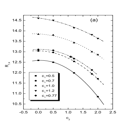
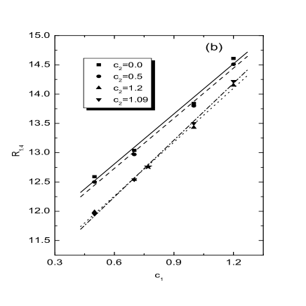
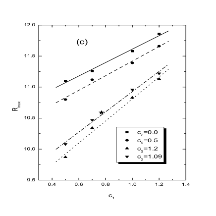
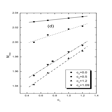
Figure 6: (a) The radius $R_{1.4}$ as a function of the second potential parameter $c_{2}$ for various values of the first potential parameter $c_{1}$. The lines correspond to the least-squares fit expressions (56) . (b) The radius $R_{1.4}$ as a function of the first potential parameter $c_{1}$ for various values of the second potential parameter $c_{2}$. The lines correspond to the least-squares fit expressions (57). (c) The radius $R_{max}$ as a function of the first potential parameter $c_{1}$ for various values of the second potential parameter $c_{1}$. The lines correspond to the least-squares fit expressions. (d) The maximum mass $M_{max}$ for various values of the second potential parameter $c_{1}$. The lines correspond to the least-squares fit expressions. In all figures the star symbol corresponds to the case $A18+\delta u+UIX^{*}$ ( $c_{1}=0.77$ and $c_{2}=1.09$)

Figure 6a illustrates the behavior of the radius $R_{1.4}$ as a function of the second potential parameter $c_{2}$ for various values of the first potential parameter $c_{1}$. The calculated points for various values of $c_{1}$ can be reproduced by a second order polynomial.

$$R_{1.4} = 12.58956+0.05378c_{2}-0.46172c_{2}^{2},\qquad c_{1}=0.5$$

$$R_{1.4} = 13.04786-0.02752c_{2}-0.32340c_{2}^{2},\qquad c_{1}=0.7$$

$$R_{1.4} = 13.85705-0.08087c_{2}-0.21393c_{2}^{2},\qquad c_{1}=1.0$$

$$R_{1.4} = 14.61946-0.19441c_{2}-0.14536c_{2}^{2},\qquad c_{1}=1.2\ .$$ (56)

In all examined cases, the radius $R_{1.4}$ is a decreasing function of the potential parameter $c_{2}$. This is a direct consequence of the softening of the equation of state due to increase of the parameter $c_{2}$.

In addition, in figure 6b the behavior of the radius $R_{1.4}$ as a function of the first potential parameter $c_{1}$ is reproduced for various values of the second potential parameter $c_{2}$. The least-squares fit values are given for the following linear equations

$$R_{1.4} = 11.09603+2.85172c_{1},\qquad c_{2}=0.0$$

$$R_{1.4} = 11.01810+2.85517c_{1},\qquad c_{2}=0.5$$

$$R_{1.4} = 10.42034+3.06724c_{1},\qquad c_{2}=1.2\ .$$ (57)

Unlike the previous case, $R_{1.4}$ is an increasing function of the potential parameter $c_{1}$. The increase of the parameter $c_{1}$ leads to the stiffness of the SE as indicated in figure 6b. It is worthwhile to note that the slopes of the best fit lines are almost the same and there is just a shift of the lines depending on the values of the parameter $c_{2}$.

Also, from figure 6a and 6b we conclude that the radius $R_{1.4}$ depends mainly on the parameter $c_{1}$ which determines the derivative of the $E_{sym}(n)$ and also the pressure $P_{sat}$ at the saturation density $n_{s}$. However, there is a small dependence on the parameter $c_{2}$ which is connected with the trend of $E_{sym}(n)$ at higher values of the density $n_{s}$. Figures 6c and 6d demonstrate the dependence of the radius $R_{max}$ and the mass $M_{max}$ respectively on the parameter $c_{1}$ (for fixed values of the parameter $c_{2}$). The star symbol corresponds the the case A18+$\delta$u+UIX^∗ ($c_{1}=0.77$ and $c_{2}=1.09$). In both cases a linear relations holds between $R_{max}$, $M_{max}$ and the parameter $c_{1}$. The lines correspond to the least-squares fit values.

It is of interest to compare the NS properties ($R_{1.4}$, $R_{max}$ and $M_{max}$) which originated from the use of equations (9) and (13). As an example we use the parameterization of equations (9) and (13) which reproduce very well the $E_{sym}$ trend of the case A18+$\delta$u+UIX^∗. As a result it is found that $R_{1.4}(c=0.9)=13.42$ and $R_{1.4}(c_{1}=0.77,c_{2}=1.09)=12.76$ (difference  5 %) , $R_{max}(c=0.9)=11$ and $R_{max}(c_{1}=0.77,c_{2}=1.09)=10.59$ (difference  3.7 %), $M_{max}(c=0.9)=1.978$ and $M_{max}(c_{1}=0.77,c_{2}=1.09)=1.974$ (difference  0.2 %). It is obvious that in the case A18+$\delta$u+UIX^∗ we receive almost identical results for $M_{max}$ while there is a small difference for $R_{1.4}$ and $R_{max}$. The differentiation of the values of $R_{1.4}$ is a consequence of the linear relation which hold between the radius $R_{1.4}$ and the derivative of the $E_{sym}$ (and consequently according to (38) to the pressure), close to the saturation point (see figures $3$ and $7$). More specifically, we receive for the two cases, $P_{s}(c=0.9)=3.83467$ MeV fm^-3 and $P_{s}(c_{1}=0.77,c_{2}=1.09)=3.48107$ MeV fm^-3. In general, the small differentiation on the radii is not surprising since the trend of equations (9) and (13), due to suitable parametrization, are similar. However, it is worth to point out that equation (13) is a generalization of equation (9), in the meaning that while equation (9) describes well the case where $E_{sym}$ is a increasing function of the density, equation (13) is sufficiently flexible to describe in addition the case where $E_{sym}$ at low densities increases along with the density and then begins to decreases although the density continues to increases.

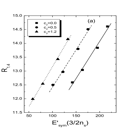
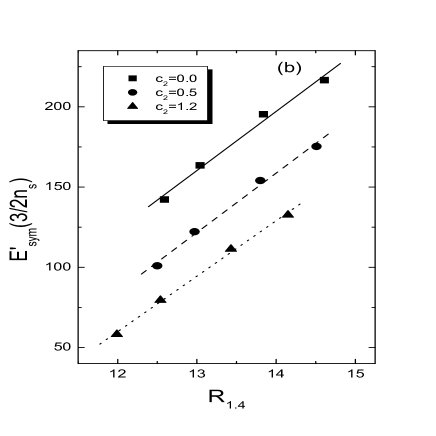
Figure 7: (a) The radius $R_{1.4}$ versus the derivative of the symmetry energy $E^{\prime}_{sym}(3n_{s}/2)$ for various values of the potential parameter $c_{2}$. (b) $E^{\prime}_{sym}(3n_{s}/2)$ versus $R_{1.4}$. The lines correspond to the least-squares fit expressions (58), (59) and (60) respectively.

To illustrate further this point, we studied the correlations between the derivative of the symmetry energy $E^{\prime}_{sym}$ and the radius $R_{1.4}$ close to the saturation point $n=3n_{s}/2$. In figure 7a we plot the radius $R_{1.4}$ versus the derivative of the symmetry energy $E^{\prime}_{sym}(3n_{s}/2)$ for fixed values of the potential parameter $c_{2}$. One can see that there is a linear relation between $R_{1.4}$ and $E^{\prime}_{sym}(3n_{s}/2)$ just like in figure 3a. The effect of the parameter $c_{2}$ is to induce a parallel shift of the best fit lines. In figure 7b we indicate the inverse relation, that means $E^{\prime}_{sym}(3n_{s}/2)$ versus $R_{1.4}$. The least-squares fit values for both cases and for various values of the parameter $c_{2}$ are given for the following equations

$$R_{1.4} = 8.70394+0.02684E_{sym}^{\prime}(3n_{s}/2),\qquad c_{2}=0$$

$$E_{sym}^{\prime}(3n_{s}/2) = -318.5026+36.82989R_{1.4}\ ,$$ (58)

$$R_{1.4} = 9.73291+0.02687E_{sym}^{\prime}(3n_{s}/2),\qquad c_{2}=0.5$$

$$E_{sym}^{\prime}(3n_{s}/2) = -359.07613+36.98138R_{1.4}\ ,$$ (59)

$$R_{1.4} = 10.27305+0.02887E_{sym}^{\prime}(3n_{s}/2),\qquad c_{2}=1.2$$

$$E_{sym}^{\prime}(3n_{s}/2) = -354.58213+34.54212R_{1.4}\ .$$ (60)

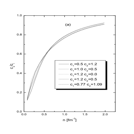
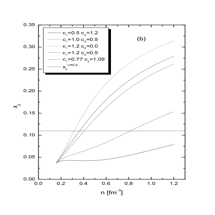
Figure 8: (a) The ratio $c_{s}/c_{l}$ versus the baryon density $n$ for various values of the potential parameters $c_{1}$ and $c_{2}$. The line for $c_{1}=0.77$ and $c_{2}=1.09$ corresponds to the case $A18+\delta u+UIX^{*}$. (b) The proton fraction $x_{p}$ versus the density $n$ for various values of the potential parameters $c_{1}$ and $c_{2}$. The line for $c_{1}=0.77$ and $c_{2}=1.09$ corresponds to the case $A18+\delta u+UIX^{*}$. The short-dotted line shows the beginning of the direct Urca process ($x_{p}=0.11$).

In figure 8a, likewise with the figure 4a we display the ratio $c_{s}/c_{l}$ as a function of the density for various cases. It is obvious that the relativistic causality is satisfied once again. In figure 8b we display the proton fraction $x_{p}$ as a function of the density for various cases. A more systematic study of the $x_{p}$ leads to the conclusion that the potential parameter $c_{1}$ plays the most critical role for the occurence of the Urca process. Specifically a higher value of the $c_{1}$ leads to the beggining Urca process in smaller values of the baryon density.

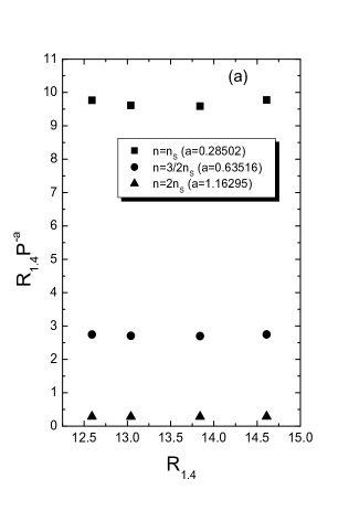
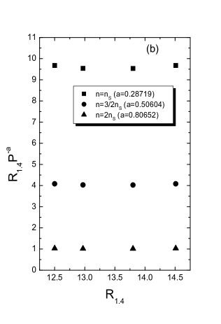
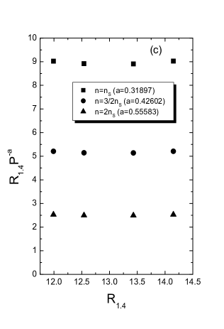
Figure 9: (a) The quantity $RP^{-a}$ as a function of the radius $R_{1.4}$ for pressure determined at $n=n_{s}$, $n=3n_{s}/2$ and $n=2n_{s}$ for $c_{2}=0$. (b) The same as before for $c_{2}=0.5$. (c) The same as before for $c_{2}=1.2$. For each density, the least-squares fit value for the exponent a is indicated.

Figure 9 illustrates the behavior of the quantity $R_{1.4}P^{-a}$ as a function of the radii $R_{1.4}$ for pressure determined at $n=n_{s}$, $3n_{s}/2$, $2n_{s}$, and also for $c_{2}=0$ (figure 9a), $c_{2}=0.5$ (figure 9b) and $c_{2}=1.2$ (figure 9c).

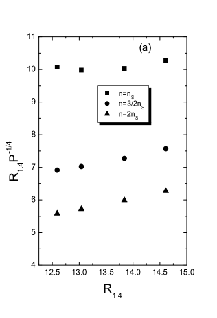
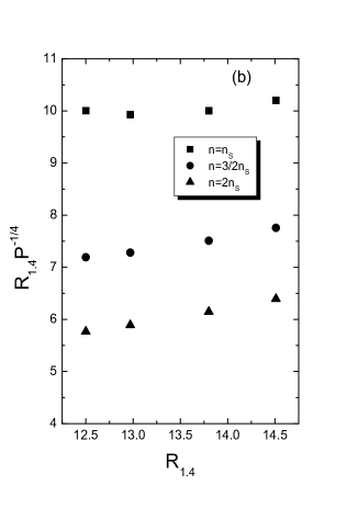
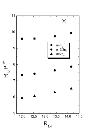
Figure 10: (a) The quantity $RP^{-1/4}$ as a function of the radius $R_{1.4}$ for pressure determined at $n=n_{s}$, $n=3n_{s}/2$ and $n=2n_{s}$ for $c_{2}=0$. (b) The same as before for $c_{2}=0.5$. (c) The same as before for $c_{2}=1.2$.

In figure 10 we plot the quantity $R_{1.4}P^{-1/4}$ as a function of $R_{1.4}$ for the pressure determined at $n=n_{s}$, $3n_{s}/2$, $2n_{s}$ and for $c_{2}=0$ (figure 10a), $c_{2}=0.5$ (figure 10b) and $c_{2}=1.2$ (figure 10c). It is obvious once again that the quantity $R_{1.4}P^{-1/4}$ is almost constant only when the pressure is calculated at the saturation point $n_{s}$. When the pressure is calculated at densities $n=3n_{s}/2$ and $n=2n_{s}$ the quantity $R_{1.4}P^{-1/4}$ is an increasing function of the radius $R_{1.4}$. Thus, as in the case of the simple parameterization of the SE, it is concluded that there is a dependence of the quantity $R_{1.4}P^{-1/4}$ from the first potential parameter $c_{1}$ as well as from the second potential parameter $c_{2}$ and consequently from the trend of the SE both for low and high values of the baryon density.

4 Summary

In the present work we performed a systematic study of the effect of the potential part of the SE on the global properties of neutron stars (masses, radii and composition). The potential part of the SE was parameterized in a generalized form both for low and high values of the baryon density in order to be efficient in reproducing the results of most microscopic calculations of dense nuclear matter.

In the case of the simple parameterization of the SE the most striking feature of our study was the derivation of a linear relation which stands between the maximum mass $M_{max}$, the radius $R_{max}$ and the radius $R_{1.4}$ with the potential parameter c. In addition, a linear relation stands between the $R_{1.4}$ and the derivative of $E^{\prime}_{sym}(n)$ for densities close to the saturation point ($n=n_{s},3n_{s}/2$). It was concluded that quantity $R_{1.4}P^{-a}$ (with $a$ and $C(n)$ fitting parameters) appears to be constant for the densities $n=n_{s},3n_{s}/2,2n_{s}$. However, the quantity $R_{1.4}P^{-1/4}$ exhibits an increasing behavior as a function of $R_{1.4}$ for $n=3n_{s}/2,n=2n_{s}$.

In the case of the more complicated parameterization, where the SE is parameterized in a different way for low and high values of the density, similar results were taken. Specifically $R_{1.4}$ is a function of both potential parameters $c_{1}$ and $c_{2}$. This means that the value of $R_{1.4}$ is affected from the density dependent trend of the SE, both in low and high densities. However, we showed that for fixed values of the parameter $c_{2}$, close to the saturation point ($n=3n_{s}/2$), a linear relation between the $R_{1.4}$ and the $E^{\prime}_{sym}(3n_{s}/2)$ stands. Finally, the quantity $R_{1.4}P^{-a}=C(n)$ appears to be constant after a suitable parameterization of the parameters $a$ and $C(n)$ but still remains dependent from the second potential parameter $c_{2}$. The quantity $R_{1.4}P^{-1/4}$, as in the previous case, exhibits an increasing behavior as a function of the $R_{1.4}$ for density values above the saturation point.

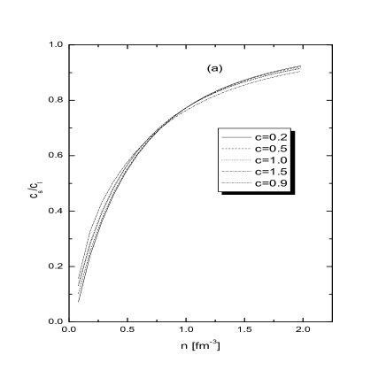
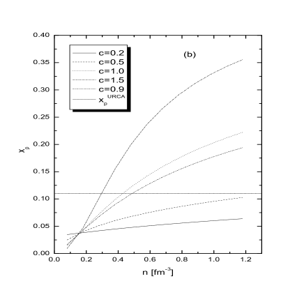
Figure 4: (a) The ratio $c_{s}/c_{l}$ versus the baryon density $n$ for various values of the potential parameter $c$. The line for $c=0.9$ corresponds to the case $A18+\delta u+UIX^{*}$. (b) The proton fraction $x_{p}$ versus the density $n$ for various values of the potential parameter $c$. The line for $c=0.9$ corresponds to the case $A18+\delta u+UIX^{*}$. The short-dotted line shows the beginning the direct Urca process ($x_{p}=0.11$).

References

- [1] M. Prakash, T.L. Ainsworth and J.M. Lattimer, Phys. Rev. Lett. 61, 2518 (1988).
- [2] J.M. Lattimer and M. Prakash, Science 304, 536 (2004).
- [3] S.L. Shapiro and S.A. Teukolsky, Black Holes, White Dwarfs and Neutron Stars: The Physics of Compact Objects (New York: Wiley) (1983).
- [4] N.K. Glendenning, Compact Stars-Nuclear Physics, Particle Physics, and General Relativity 2nd edn (New York: Springer) (2000).
- [5] F. Weber, Pulsars as Astrophysical Laboratories for Nuclear and Particle Physics (Bristol: Institute of Physics Publishing) (1999).
- [6] M. Prakash, The Equation of State and Neutron Star lectures delivered at the Winter School held in Puri India (1994).
- [7] H. Heiselberg and M. Hjorth-Jensen, Phys. Rep. 328, 237 (2000).
- [8] A.W. Steiner, M. Prakash, J.M. Lattimer and P.J. Ellis, Phys. Rep. 411, 325 (2005).
- [9] Madappa Prakash, I. Bombaci, Manju Prakash, P.J. Ellis, J.M. Lattimer and R. Knorren, Phys. Rep. 280, 1 (1997).
- [10] J.M. Lattimer and M. Prakash, Phys. Rep. 333-334, 121 (2000).
- [11] G.S. Sahakian, Equilibrium configurations of degenerate gaseous masses Halsten, Wiley, New York, Israel program from scientific translations, Jerusalem (1974).
- [12] R.C. Tolman, Phys. Rev. 55, 364 (1939).
- [13] J.R. Oppenheimer and G.M. Volkov, Phys. Rev. 55, 374 (1939).
- [14] A.E.L. Dieperink, Y. Dewulf, D. Van Neck, M. Waroquier and V. Rodin, Phys. Rev. C 68, 064307 (2003).
- [15] A.E.L. Dieperink and D. Van Neck, Journ. of Phys., Conf. Series 20, 160 (2005).
- [16] J.R. Stone, P.D. Stevenson, J.C. Miller and M.R. Strayer, Phys. Rev. C 65, 064312 (2002).
- [17] J.R. Stone, J.C. Miller, R. Koncewicz, P.D. Stevenson and M.R. Strayer, Phys. Rev. C 68, 034324 (2003).
- [18] J.R. Stone and P.G. Reinhard, Progr. Part. Nucl Phys. 58, 587 (2007).
- [19] D.V. Shetty, S.J. Yennello and G.A. Souliotis, Phys. Rev. C 75, 034602 (2007).
- [20] D.V. Shetty, S.J. Yennello, A.S. Botvina and G.A. Souliotis, nucl-ex/0603016.
- [21] T. Klähn et al., Phys. Rev. C 74, 035802 (2006).
- [22] P. Danielewicz, Nucl. Phys. A 727, 233 (2003).
- [23] P. Danielewicz, nucl-th/0607030.
- [24] P. Danielewicz P, nucl-th/0411115.
- [25] R.B. Wiringa, V. Fiks and A. Fabrocini, Phys. Rev. C 38, 1010 (1988).
- [26] Q. Li, Z. Li, S. Soff, R.K. Gupta, M. Bleicher and H.J. Stocker, J. Phys. G: Nucl. Part. Phys. 31, 1359 (2005).
- [27] W. Zuo, A. Lejeune, U. Lombardo and J.F. Mathiot, Eur. Phys. J. A 14, 469 (2002).
- [28] F. Douchin and P. Haensel, Astr. and Astroph. 380, 151 (2001).
- [29] M. Baldo, I. Bombaci and G.F. Burgio, Astr. and Astroph. 328, 274 (1997).
- [30] C.H. Lee, T.T.S. Kuo, G.Q. Li and G.E. Brown, Phys. Rev. C 57, 3488 (1998).
- [31] B. Liu, H. Guo, V. Creco, U. Lombardo, M. Di Toro and Cai-Dian Lu, Eur. Phys. J. A 22, 337 (2004).
- [32] P.G. Krastev and F. Sammarruca, Phys. Rev. C 74, 025808 (2006).
- [33] B.A. Li and W. Udo. Schröder, Isospin Physics in Heavy-Ion Collisions at Intermediate Energies (New York: Nova Science) (2001).
- [34] B.A. Li and A.W. Steiner, Phys. Lett. B 642, 436 (2006).
- [35] B.A. Li, C.B. Das, S.D. Gupta and C. Gale, Phys. Rev. C 69 (R), 011603 (2004).
- [36] D. Vretenar, T. Niks̆ić and P. Ring, Phys. Rev. C 68, 024310 (2003).
- [37] J.M. Lattimer and M. Prakash, Astrophys. J. 550, 426 (2001).
- [38] A. Akmal and V.R. Pandharipande, Phys. Rev. C 56, 2261 (1997).
- [39] A. Akmal, V.R. Pandharipande and D.G. Ravenhall, Phys. Rev. C 58, 1804 (1998).
- [40] J. Morales, V.R. Pandharipande and D.G. Ravenhall, Phys. Rev. C 66, 054308 (2002).
- [41] X.R. Zhou, G.F. Burgio, U. Lombardo, H.J. Schulze and W. Zuo, Phys. Rev. C 69, 018801 (2004).
- [42] L.W. Chen, C.M. Ko and B.A. Li, Phys. Rev. Lett. 94, 032701 (2005).
- [43] B.A. Li and L.W. Chen, Phys. Rev. C 72, 064611 (2005).
- [44] A.W. Steiner and B.A. Li, Phys. Rev. C 72 (R), 041601 (2005).
- [45] L.W. Chen, C.M. Ko and B.A. Li, Phys. Rev. C 72, 064309 (2005).
- [46] J.M. Lattimer, J. Phys. G: Nucl. Part. Phys. 30, S479 (2004).
- [47] C. J. Pethick, Rev. Mod. Phys. 64, 1133 (1992).
- [48] J.M. Lattimer, C.J. Pethick, M. Prakash and P. Haensel, Phys. Rev. Lett. 66, 2701 (1991).
- [49] L.Sh. Grigoryan and G.S. Sahakian, Astrophys. Space Sci. 95, 305 (1983).
- [50] R.P. Feynman, N. Metropolis and E. Teller, Phys. Rev. 75, 1561 (1949).
- [51] G. Baym, C. Pethik and P. Sutherland, Astroph. J. 170, 299 (1971).