Abstract

A $\gamma$-soft analogue of the confined $\beta$-soft (CBS) rotor model is developed, by using a $\gamma$-independent displaced infinite well $\beta$-potential in the Bohr Hamiltonian, for which exact separation of variables is possible. Level schemes interpolating between the E(5) critical point symmetry (with $R_{4/2}=E(4_{1}^{+})/E(2_{1}^{+})=2.20$) and the O(5) $\gamma$-soft rotor (with $R_{4/2}=2.50$) are obtained, exhibiting a crossover of excited $0^{+}$ bandheads which leads to agreement with the general trends of $0_{2}^{+}$ states in this region and is observed experimentally in ^128,130Xe.

1 Introduction

Critical point symmetries [1, 2], related to shape/phase transitions, have attracted recently considerable attention in nuclear structure, since they provide parameter-free (up to overall scale factors) predictions supported by experimental evidence [3, 4, 5, 6]. The E(5) critical point symmetry [1], in particular, is related to the shape/phase transition between vibrational [U(5)] and $\gamma$-unstable [O(6)] nuclei, while X(5) [2] is related to the transition between vibrational and axially symmetric prolate [SU(3)] nuclei. A systematic study of phase transitions in nuclear collective models has been given in [7, 8, 9].

In both the E(5) and X(5) models, exact [in E(5)] or approximate [in X(5)] separation of the $\beta$ and $\gamma$ collective variables of the Bohr Hamiltonian [10] is achieved, and an infinite square well potential in $\beta$ is used. (Various analytic solutions of the Bohr Hamiltonian have been recently reviewed in Ref. [11], while a recently introduced [12, 13, 14] computationally tractable version of the Bohr collective model is already in use [15]. ) Models interpolating between E(5) [or X(5)] and U(5) have been obtained by using $\beta^{2n}$ potentials (with $n=1$, 2, 3, 4) in the relevant [E(5) or X(5)] framework [16, 17, 18], while an interpolation between X(5) and the rigid rotor limit has been achieved in the framework of the confined $\beta$-soft (CBS) rotor model [19], by using in the X(5) framework infinite square well potentials in $\beta$ with boundaries $\beta_{M}>\beta_{m}\geq 0$, with the case of $\beta_{m}=0$ corresponding to the original X(5) model. The CBS rotor model showed considerable success in describing transitional and strongly deformed nuclei in the rare earths and actinides [20, 21].

In the present work an interpolation between E(5) and the $\gamma$-soft rotor [O(5)] limit is achieved, by using in the E(5) framework $\gamma$-independent infinite square well potentials in $\beta$ with boundaries $\beta_{M}>\beta_{m}\geq 0$. The model contains one free parameter, $r_{\beta}=\beta_{m}/\beta_{M}$, the case with $r_{\beta}=0$ corresponding to the original E(5) model, while $r_{\beta}\to 1$ leads to the $\gamma$-soft rotor [O(5)] limit. A special case with the two lowest excited $0^{+}$ states being degenerate occurs for $r_{\beta_{c}}=0.171$. Experimental examples on the E(5) side and on the O(5) side of $r_{\beta_{c}}$ are found to correspond to ¹³⁰Xe and ¹²⁸Xe, respectively. The crossover of $0^{+}$ bandheads observed at $r_{\beta_{c}}$ is important in reproducing the experimental trends of $0_{2}^{+}$ bandheads in the $R_{4/2}=E(4_{1}^{+})/E(2_{1}^{+})$ region between 2.20 [E(5)] and 2.50 [O(5)].

In Section 2 the calculation of the energy spectra and $B(E2)$ transition rates is decribed, while results are shown and compared to experiment in Section 3. An overall discussion of the present results in given in Section 4.

2 The model

We consider the Bohr Hamiltonian [10]

$$H=-\frac{\hbar^{2}}{2B}\Bigl{[}\Delta_{R}+\frac{1}{\beta^{2}}\Delta_{\Omega}\Bigr{]}+U(\beta),$$ (1)

with

$$\Delta_{R} = \frac{1}{\beta^{4}}\frac{\partial}{\partial\beta}\beta^{4}\frac{\partial}{\partial\beta}=\frac{\partial^{2}}{\partial\beta^{2}}+\frac{4}{\beta}\frac{\partial}{\partial\beta},$$ (2)

$$\Delta_{\Omega} = \frac{1}{\sin 3\gamma}\frac{\partial}{\partial\gamma}\sin 3\gamma\frac{\partial}{\partial\gamma}-\sum_{k=1}^{3}\frac{L_{k}^{\prime 2}(\theta_{i})}{4\sin^{2}(\gamma-\frac{2\pi}{3}k)},$$ (3)

where $\beta$ and $\gamma$ are the usual collective coordinates, $L_{k}^{\prime}$ ($k=1,2,3$) are the components of angular momentum in the intrinsic frame, $\theta_{i}$ ($i=1,2,3$) are the Euler angles, and $B$ is the mass parameter. The potential $U(\beta)$ depends only on the collective coordinate $\beta$ [22].

Using the factorized wave function $\Psi(\beta,\gamma,\theta_{i})=F(\beta)\Phi(\gamma,\theta_{i})$ [1, 22] the Schrödinger equation corresponding to the Hamiltonian (1) is separated into two parts:

(a) The angular part

$$-\Delta_{\Omega}\Phi(\gamma,\theta_{i})=\tau(\tau+3)\Phi(\gamma,\theta_{i}),$$ (4)

where $\tau$ is the seniority quantum number and $\Delta_{\Omega}$ is a quadratic invariant operator of the group SO(5) [22, 23]. A detailed discussion can be found in Ref. [23].

(b) The radial part

$$\frac{d^{2}F(\beta)}{d\beta^{2}}+\frac{4}{\beta}\frac{dF(\beta)}{d\beta}+\left[\frac{2B}{\hbar^{2}}\Bigl{(}E-U(\beta)\Bigr{)}-\frac{\tau(\tau+3)}{\beta^{2}}\right]F(\beta)=0.$$ (5)

In the radial equation (5) we consider an infinite well potential [1, 22] confined between boundaries [19] at $\beta_{m}$ and $\beta_{M}$ ($0<\beta_{m}<\beta_{M}$)

$$U(\beta)=\left\{\begin{array}[]{ll}0&,\quad\beta_{m}\leq\beta\leq\beta_{M}\\ \infty&,\quad 0\leq\beta<\beta_{m},\quad\beta>\beta_{M}.\end{array}\right.$$ (6)

Defining $k^{2}=2BE/\hbar^{2}$ and substituting $F(\beta)=\beta^{-3/2}P(\beta)$, Eq. (5) in the interval $\beta\in[\beta_{m},\beta_{M}]$ takes the form of a Bessel equation of $\nu$th order

$$\beta^{2}P^{\prime\prime}(\beta)+\beta P^{\prime}(\beta)+\bigl{(}k^{2}\beta^{2}-\nu^{2}\bigr{)}P(\beta)=0,$$ (7)

where $\nu=\tau+3/2$. The boundary conditions at $\beta_{m}$ and $\beta_{M}$ are

$$P(\beta_{m})=0,\qquad P(\beta_{M})=0,\qquad 0<\beta_{m}<\beta_{M}.$$ (8)

The general solution of Eq. (7) is the cylindrical function

$$P(\beta)=aJ_{\nu}(k\beta)+bY_{\nu}(k\beta),$$ (9)

where $J_{\nu}(z)$ and $Y_{\nu}(z)$ are the Bessel functions of the first and second kind respectively of order $\nu=\tau+3/2$, and ($a,b$) are constants to be determined. The boundary conditions (8) lead to a homogenous system for ($a,b$)

$$aJ_{\nu}(k\beta_{M})+bY_{\nu}(k\beta_{M})=0,$$

$$aJ_{\nu}(k\beta_{m})+bY_{\nu}(k\beta_{m})=0,$$

which has nontrivial solutions in ($a,b$) if its determinant is set to vanish

$$J_{\nu}(k\beta_{M})Y_{\nu}(k\beta_{m})-J_{\nu}(k\beta_{m})Y_{\nu}(k\beta_{M})=0.$$ (10)

In this way the boundary conditions (8) lead to a discrete spectrum of the parameter $k$, the values of which are the positive roots of Eq. (10). Eq. (10) can be written in the form [19]

$$J_{\nu}(x)Y_{\nu}(r_{\beta}x)-J_{\nu}(r_{\beta}x)Y_{\nu}(x)=0,$$ (11)

where $x=k\beta_{M}$ and the parameter $r_{\beta}$ denotes the ratio $r_{\beta}=\beta_{m}/\beta_{M}$. Here we consider the case in which the parameter $\beta_{M}$ is fixed and $\beta_{m}$ varies in the range $0<\beta_{m}<\beta_{M}$, the ratio $r_{\beta}$ taking values in the interval $0<r_{\beta}<1$.

Let $x_{\xi\tau}^{(r_{\beta})}$ be the $\xi$th positive root of Eq. (11), and respectively $k_{\xi\tau}^{(r_{\beta})}=x_{\xi\tau}^{(r_{\beta})}/\beta_{M}$ be the $\xi$th positive root of Eq. (10), where $\nu=\tau+3/2$. Then the normalized eigenfunctions $P_{\xi\tau}^{(r_{\beta})}(\beta)$ can be represented in the form

$$P_{\xi\tau}^{(r_{\beta})}(\beta)=\left[A_{\xi\tau}^{(r_{\beta})}\right]^{-1/2}\Bigl{[}J_{\nu}(k_{\xi\tau}^{(r_{\beta})}\beta)Y_{\nu}(k_{\xi\tau}^{(r_{\beta})}\beta_{m})-J_{\nu}(k_{\xi\tau}^{(r_{\beta})}\beta_{m})Y_{\nu}(k_{\xi\tau}^{(r_{\beta})}\beta)\Bigr{]},$$ (12)

where $\beta_{m}\leq\beta\leq\beta_{M}$ and $k_{\xi\tau}^{(r_{\beta})}\beta_{m}=r_{\beta}x_{\xi\tau}^{(r_{\beta})}$. Then the normalized solutions of Eq. (5) in the interval $[\beta_{m},\beta_{M}]$ are

$$F_{\xi\tau}^{(r_{\beta})}(\beta)=\beta^{-3/2}P_{\xi\tau}^{(r_{\beta})}(\beta).$$ (13)

The constants $A_{\xi\tau}^{(r_{\beta})}$ in (12) are obtained from the normalization condition

$$\int_{\beta_{m}}^{\beta_{M}}\beta^{4}\left[F_{\xi\tau}^{(r_{\beta})}(\beta)\right]^{2}\,d\beta=\int_{\beta_{m}}^{\beta_{M}}\beta\left[P_{\xi\tau}^{(r_{\beta})}(\beta)\right]^{2}\,d\beta=1.$$ (14)

The corresponding energy spectrum is

$$E_{\xi\tau}(r_{\beta})=\frac{\hbar^{2}}{2B}\,\left[k_{\xi\tau}^{(r_{\beta})}\right]^{2}=\frac{\hbar^{2}}{2B\beta_{M}^{2}}\,\left[x_{\xi\tau}^{(r_{\beta})}\right]^{2}.$$ (15)

In the limiting case of $\beta_{m}\to 0$ (or $r_{\beta}\to 0$) the spectrum and eigenfunctions correspond to the E(5) critical point symmetry [1].

The factorized wave functions are denoted by

$$|r_{\beta};\xi\tau\mu LM\rangle\equiv\Psi_{\xi\tau\mu LM}^{(r_{\beta})}(\beta,\gamma,\theta_{i})=F_{\xi\tau}^{(r_{\beta})}(\beta)\Phi^{\tau\mu}_{LM}(\gamma,\theta_{i}),$$ (16)

where $\tau$ is the seniority quantum number, $\mu=0,1,2,\ldots,[\tau/3]$, and for a given value of $\mu$ the angular momentum $L$ takes values $L=2\rho,2\rho-2,2\rho-3,\ldots,\rho+1,\rho$, where $\rho=\tau-3\mu$. The angular part of the wave function has the form [24]

$$\Phi^{\tau\mu}_{LM}(\gamma,\theta_{i})=N_{\tau\mu L}^{-1/2}\sqrt{\frac{2L+1}{8\pi^{2}}}\sum_{K}\phi^{\tau\mu}_{LK}(\gamma)D_{MK}^{L\ast}(\theta_{i}),$$ (17)

where $N_{\tau\mu L}$ is a normalization constant and the index $K$ in the above sum takes even values in the interval $|K|\leq L$. In the present case we consider only states which are non-degenerate with respect to the quantum number $L$ in the framework of the group embedding SO(5)$\supset$SO(3).

The reduced transition probabilities $B(E2)$ for the $E2$ transitions

$$B(E2;\alpha_{i}L_{i}\to\alpha_{f}L_{f})=\frac{|\langle\alpha_{f}L_{f}\|T^{(E2)}\|\alpha_{i}L_{i}\rangle|^{2}}{2L_{i}+1},$$ (18)

are calculated for the quadrupole operator $T^{(E2)}$ proportional to the collective variable $\alpha_{m}$

$$T^{(E2)}_{m}\propto\beta\Bigr{[}D^{2\ast}_{m0}(\theta_{i})\cos\gamma+\frac{1}{\sqrt{2}}\bigl{(}D^{2\ast}_{m2}(\theta_{i})+D^{2\ast}_{m-2}(\theta_{i})\bigr{)}\sin\gamma\Bigr{]}.$$ (19)

As a result for the $E2$ transitions one has

$$B(E2;L_{\xi\tau\mu}\to L^{\prime}_{\xi^{\prime}\tau^{\prime}\mu^{\prime}})=R^{2}_{\xi^{\prime}\tau^{\prime};\,\xi\tau}(r_{\beta})\,G^{2}_{\tau^{\prime}\mu^{\prime}L^{\prime};\,\tau\mu L},$$ (20)

where

$$R_{\xi^{\prime}\tau^{\prime};\,\xi\tau}(r_{\beta})=\int_{\beta_{m}}^{\beta_{M}}\beta F_{\xi^{\prime}\tau^{\prime}}^{(r_{\beta})}(\beta)F_{\xi\tau}^{(r_{\beta})}(\beta)\,\beta^{4}d\beta,$$ (21)

and $G_{\tau^{\prime}\mu^{\prime}L^{\prime};\,\tau\mu L}$ are geometrical factors corresponding to the embedding SO(5)$\supset$SO(3). The selection rules for the matrix elements of the quadrupole operator $T^{(E2)}_{m}$ defined in (19) are $|\Delta\tau|=1$ and $|\Delta L|\leq 2$. We stress that all wave functions, energy eigenvalues, and transition matrix elements are exact analytical solutions of the Bohr Hamiltonian for the class of potentials considered here.

3 Analytical results and comparison to experiment

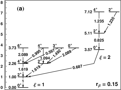
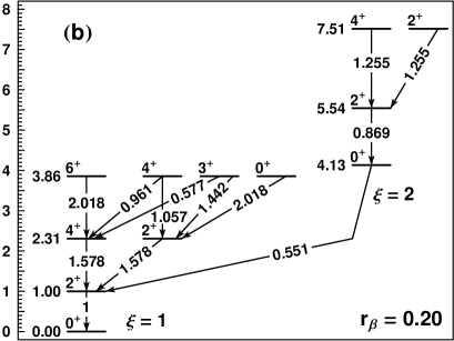
Figure 1: Energy levels (normalized to the excitation energy of the $2_{1}^{+}$ state) and $B(E2)$ values (normalized to $B(E2;2_{1}^{+}\to 0_{1}^{+})$) for two different values of the structural parameter $r_{\beta}=\beta_{m}/\beta_{M}$ around the $0^{+}_{2,3}$ crossing.

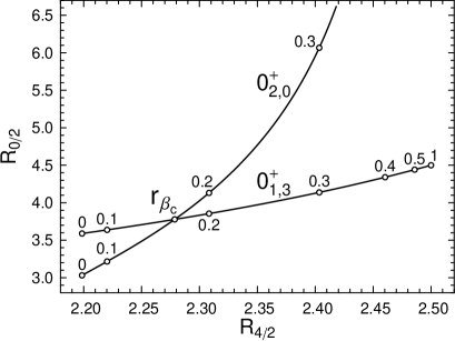
Figure 2: Energy of $0^{+}$ states (normalized to the energy of the $2_{1}^{+}$ state), labeled as $R_{0/2}$, vs. the ratio $R_{4/2}=E(4_{1}^{+})/E(2_{1}^{+})$. The parameter $r_{\beta}$ on each curve starts from zero at the left end, increasing to the right. The crossover of the ($\xi=2$, $\tau=0$, $L=0$) and the ($\xi=1$, $\tau=3$, $L=0$) curves occurs at $r_{\beta_{c}}\approx 0.171263$, $(R_{4/2},\ R_{0/2})_{c}\approx(2.27861,\ 3.77797)$.

Analytical results for energy levels and $B(E2)$ transition rates are shown in Fig. 1 . The main observation regards the position of the lowest excited $0^{+}$ states. In E(5) [1] and for low values of $r_{\beta}<r_{\beta_{c}}=0.171$, $0_{2}^{+}$ corresponds to ($\xi=2$, $\tau=0$), while $0_{3}^{+}$ is provided by ($\xi=1$, $\tau=3$). For higher values of $r_{\beta}>r_{\beta_{c}}=0.171$ the picture is opposite, with $0_{2}^{+}$ corresponding to ($\xi=1$, $\tau=3$), and $0_{3}^{+}$ given by ($\xi=2$, $\tau=0$). The latter eigenstate is shifted toward infinite energy as the O(5) limit is approached for $r_{\beta}\to 1$. The normalized $0^{+}$ bandheads are shown as a function of the $R_{4/2}=E(4_{1}^{+})/E(2_{1}^{+})$ ratio in Fig. 2. On each curve the parameter $r_{\beta}$ starts from $r_{\beta}=0$ on the left, gradually increasing to the right. The crossover of the ($\xi=2$, $\tau=0$) and the ($\xi=1$, $\tau=3$) curves occurs at $r_{\beta_{c}}=0.171$.

The existence of the $0^{+}$ state’s crossover is crucial in keeping the model predictions in agreement with the general trends shown by the experimental $R_{0/2}=E(0_{2}^{+})/E(2_{1}^{+})$ ratio as a function of the $R_{4/2}=E(4_{1}^{+})/E(2_{1}^{+})$ ratio, given in Ref. [25]. In the region with $2.20<R_{4/2}<2.50$, covered by the present model, the experimental $R_{0/2}$ values stay indeed below 5.0, in agreement with what is seen in Fig. 2 for the ($\xi=1$, $\tau=3$) bandhead.

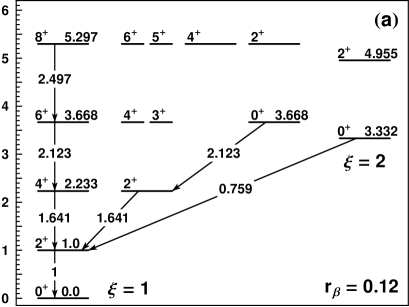
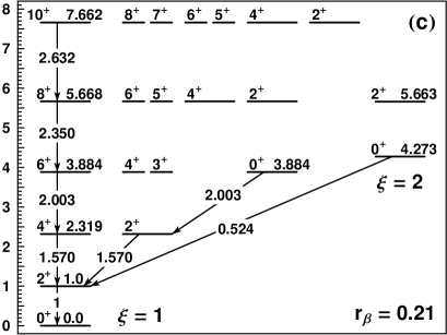
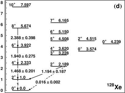
Figure 3: Comparison of the model predictions for $r_{\beta}=0.12$ (a) to the experimental data of ¹³⁰Xe [26] (b), and of the model predictions for $r_{\beta}=0.21$ (c) to the experimental data for ¹²⁸Xe [27] (d).

It is interesting to identify nuclei corresponding to parameter values near the region $r_{\beta}=0.15$-0.20, in which the crossover of the $0^{+}$ bandheads occurs. Below $r_{\beta_{c}}=0.171$ the situation resembles the one in E(5), with $6_{1}^{+}$, $4_{2}^{+}$ and $0_{3}^{+}$ states being nearly degenerate, while the $0_{2}^{+}$ state lies lower than them. Beyond $r_{\beta_{c}}=0.171$ the near degeneracy applies to the $6_{1}^{+}$, $4_{2}^{+}$ and $0_{2}^{+}$ states, while the $0_{3}^{+}$ state lies higher than them. This situation occurs in the neighboring nuclei ¹³⁰Xe (corresponding to $r_{\beta}=0.12$) and ¹²⁸Xe (reproduced by $r_{\beta}=0.21$), shown in Fig. 3. (The parameter $r_{\beta}$ has been fitted to the experimental $R_{4/2}$ ratio of each nucleus.) In the latter case, known $B(E2)$ values, too, agree remarkably well with the theoretical predictions.

Both before and after the crossover, the $0^{+}$ bandhead with ($\xi=1$, $\tau=3$) is connected by a strong $E2$ transition to the $2_{2}^{+}$ state, while the $0^{+}$ bandhead with ($\xi=2$, $\tau=0$) decays less strongly to the $2_{1}^{+}$ level. These interband $B(E2)$ values provide a stringent test to the model. However, their absolute values are unknown experimentally.

It is nevertheless possible to unambiguously characterize the predominant nature of the two excited $0^{+}_{2,3}$ states of ^128,130Xe by considering their $E2$ decay branching ratios to the lowest two $2^{+}_{1,2}$ states. We thus define the double-ratio

$${\cal Z}(0^{+}_{3/2}) = \frac{B(E2;0^{+}_{3}\to 2^{+}_{2})/B(E2;0^{+}_{3}\to 2^{+}_{1})}{B(E2;0^{+}_{2}\to 2^{+}_{2})/B(E2;0^{+}_{2}\to 2^{+}_{1})}$$ (22)

$$= \frac{\left(\frac{E_{\gamma}(0^{+}_{3}\to 2^{+}_{1})}{E_{\gamma}(0^{+}_{3}\to 2^{+}_{2})}\right)^{5}\frac{I_{\gamma}(0^{+}_{3}\to 2^{+}_{2})}{I_{\gamma}(0^{+}_{3}\to 2^{+}_{1})}}{\left(\frac{E_{\gamma}(0^{+}_{2}\to 2^{+}_{1})}{E_{\gamma}(0^{+}_{2}\to 2^{+}_{2})}\right)^{5}\frac{I_{\gamma}(0^{+}_{2}\to 2^{+}_{2})}{I_{\gamma}(0^{+}_{2}\to 2^{+}_{1})}}$$ (23)

for which one expects values $>1$ for $r_{\beta}<r_{\beta_{c}}$ and $<1$ for $r_{\beta}>r_{\beta_{c}}$, respectively. Eq. (23) involves $\gamma$-ray energies and intensity ratios. The data [26, 27, 28] yield values of ${\cal Z}(0^{+}_{3/2})=52\pm 30$ for ¹³⁰Xe and ${\cal Z}(0^{+}_{3/2})=0.32\pm 0.17$ for ¹²⁸Xe, as given on Table 1. The experimental values for ¹³⁰Xe and ¹²⁸Xe differ by two orders of magnitude. Despite the large uncertainties that originate in the 50% uncertainty for the low intensity of the initially forbidden $0^{+}\to 2^{+}_{2}$ low-energy transition [26, 27, 28], the data prove the crossing of the different $0^{+}$ configurations with ($\xi=2$, $\tau=0$) and ($\xi=1$, $\tau=3$) between ¹³⁰Xe and ¹²⁸Xe, as predicted by the model from a fit to the relative $4^{+}_{1}$ excitation energy $R_{4/2}$.

Having identified the $0^{+}$ configuration crossing we can analyze it quantitatively in a two-state mixing scenario. These close-lying experimental $0^{+}$ states are considered as an orthogonal mixture of the crossing model states $0^{+}_{2}=\alpha_{2}0^{+}_{\xi=2,\tau=0}+\alpha_{3}0^{+}_{\xi=1,\tau=3}$ and $0^{+}_{3}=-\alpha_{3}0^{+}_{2,0}+\alpha_{2}0^{+}_{1,3}$ due to residual interactions not accounted for by the simple model. This yields ${\cal Z}(0^{+}_{3/2})=(\alpha_{2}/\alpha_{3})^{4}$ due to the $\tau$-selection rules for the $E2$ operator in the unperturbed situation and allows for the mixing coefficients to be determined. The squared amplitudes $\alpha_{2}^{2}$ quantify the $0^{+}$ configuration crossing. The contribution of the $0^{+}_{\xi=2,\tau=0}$ model state to the observed $0^{+}_{2}$ state drops from 88(3)% in ¹³⁰Xe to 43(3)% in ¹²⁸Xe as displayed in Table 1.

With that information a further test of the model prediction for $E2$ transition rates can be performed assuming only the validity of the two-state-mixing scenario. The relative strengths of the unperturbed interband $E2$ transitions can be extracted from the experimental $E2$ branching ratios

$$\left[\frac{B(E2;0^{+}_{1,3}\to 2^{+}_{2})}{B(E2;0^{+}_{2,0}\to 2^{+}_{1})}\right]_{\rm unperturbed}$$

$$= \left(\frac{\alpha_{3}}{\alpha_{2}}\right)^{2}\left[\frac{B(E2;0^{+}_{3}\to 2^{+}_{2})}{B(E2;0^{+}_{3}\to 2^{+}_{1})}\right]_{\rm expt}$$

$$= \sqrt{\frac{\frac{I_{\gamma}(0^{+}_{2}\to 2^{+}_{2})}{I_{\gamma}(0^{+}_{2}\to 2^{+}_{1})}\left(\frac{E_{\gamma}(0^{+}_{2}\to 2^{+}_{1})}{E_{\gamma}(0^{+}_{2}\to 2^{+}_{2})}\right)^{5}}{\frac{I_{\gamma}(0^{+}_{3}\to 2^{+}_{1})}{I_{\gamma}(0^{+}_{3}\to 2^{+}_{2})}\left(\frac{E_{\gamma}(0^{+}_{3}\to 2^{+}_{2})}{E_{\gamma}(0^{+}_{3}\to 2^{+}_{1})}\right)^{5}}}$$

The rhs involves $E2$ intensity ratios in the perturbed (experimental) situation. The experimental values (rhs) are compared to the theoretical values for the lhs of Eq. (3) at the bottom of Table 1. The data on ¹²⁸Xe coincide with the model within the uncertainties. The data on ¹³⁰Xe also exhibit the predicted dominance of the $B(E2;0^{+}_{1,3}\to 2^{+}_{2})$ value over the $B(E2;0^{+}_{2,0}\to 2^{+}_{2})$ value but by an order of magnitude more pronounced than theoretically expected. This numerical deviation calls for better data on the weak $0^{+}_{2}\to 2^{+}_{2}$ 672-keV decay intensity with its present uncertainty of 50% [28].

4 Summary

A $\gamma$-soft analogue of the confined $\beta$-soft (CBS) rotor model has been constructed and exactly solved analytically, by using a $\gamma$-independent displaced infinite well $\beta$-potential in the Bohr equation, in which exact separation of variables is possible in this case. The model obtained contains one free parameter, the ratio $r_{\beta}=\beta_{m}/\beta_{M}$ of the positions of the left wall ($\beta_{m}$) and the right wall ($\beta_{M}$) of the potential well, and interpolates between the E(5) critical point symmetry, possessing $R_{4/2}=E(4_{1}^{+})/E(2_{1}^{+})=2.20$ and obtained for $r_{\beta}=0$, and the $\gamma$-soft rotor O(5), having $R_{4/2}=2.50$ and obtained for $r_{\beta}\to 1$. Due to the explicit O(5) symmetry the model might be addressed as the O(5)-Confined $\beta$-Soft Rotor Model [O(5)-CBS]. A crossover of excited $0^{+}$ bandheads as a function of $R_{4/2}$ is predicted, which is crucial in keeping the model predictions for the $0_{2}^{+}$ bandhead in good agreement with experimental systematics in this region of $R_{4/2}$ ratios. This crossover is manifested in ^128,130Xe as is seen quantitatively from experimental $E2$ decay intensity ratios. Information on relative and absolute $E2$ transitions in ¹²⁸Xe are in good agreement with the model predictions when simple configuration mixing is accounted for, while more accurate experimental information on $B(E2)$s in ¹³⁰Xe is desirable for further significant tests of the model.

Table 1: Comparison of data [26, 27, 28] on ^130,128Xe to the model [O(5)-CBS] and the two-state mixing scenario (see Section 3).

  ¹³⁰Xe O(5)-CBS ¹²⁸Xe O(5)-CBS $r_{\beta}=0.12$ $r_{\beta}=0.21$ ${\cal Z}(0^{+}_{3/2})$ 52(30) $\infty$ 0.32(17) 0 $\alpha_{2}^{2}$ 0.88(3) – 0.43(3) – $\frac{B(E2;0^{+}_{1,3}\to 2^{+}_{2})}{B(E2;0^{+}_{2,0}\to 2^{+}_{1})}$ 28(9) 2.8 3.7(1.0) 3.8

References

• [1] F. Iachello, Phys. Rev. Lett. 85, 3580 (2000).
• [2] F. Iachello, Phys. Rev. Lett. 87, 052502.
• [3] R. F. Casten and N. V. Zamfir, Phys. Rev. Lett. 85, 3584 (2000).
• [4] R. F. Casten and N. V. Zamfir, Phys. Rev. Lett. 87, 052303 (2001).
• [5] R. M. Clark, M. Cromaz, M. A. Deleplanque, M. Descovich, R. M. Diamond, P. Fallon, I. Y. Lee, A. O. Macchiavelli, H. Mahmud, E. Rodriguez-Vieitez, F. S. Stephens, and D. Ward, Phys. Rev. C 69, 064322 (2004).
• [6] R. M. Clark, M. Cromaz, M. A. Deleplanque, M. Descovich, R. M. Diamond, P. Fallon, R. B. Firestone, I. Y. Lee, A. O. Macchiavelli, H. Mahmud, E. Rodriguez-Vieitez, F. S. Stephens, and D. Ward, Phys. Rev. C 68, 037301 (2003).
• [7] D. J. Rowe, Nucl. Phys. A 745, 47 (2004).
• [8] P. S. Turner and D. J. Rowe, Nucl. Phys. A 756, 333 (2005).
• [9] G. Rosensteel and D. J. Rowe, Nucl. Phys. A 759, 92 (2005).
• [10] A. Bohr, Mat. Fys. Medd. K. Dan. Vidensk. Selsk. 26, 14 (1952).
• [11] L. Fortunato, Eur. Phys. J. A 26, s01, 1 (2005).
• [12] D. J. Rowe, Nucl. Phys. A 735, 372 (2004).
• [13] D. J. Rowe, P. S. Turner, and J. Repka, J. Math. Phys. 45, 2761 (2004).
• [14] D. J. Rowe and P. S. Turner, Nucl. Phys. A 753, 94 (2005).
• [15] M. A. Caprio, Phys. Rev. C 72, 054323 (2005).
• [16] J. M. Arias, C. E. Alonso, A. Vitturi, J. E. GarcΓ­a-Ramos, J. Dukelsky, and A. Frank, Phys. Rev. C 68, 041302 (2003).
• [17] D. Bonatsos, D. Lenis, N. Minkov, P. P. Raychev, and P. A. Terziev, Phys. Rev. C 69, 044316 (2004).
• [18] D. Bonatsos, D. Lenis, N. Minkov, P. P. Raychev, and P. A. Terziev, Phys. Rev. C 69, 014302 (2004).
• [19] N. Pietralla and O. M. Gorbachenko, Phys. Rev. C 70, 011304 (2004).
• [20] K. Dusling and N. Pietralla, Phys. Rev. C 72, 011303 (2005).
• [21] K. Dusling, N. Pietralla, G. Rainovski, T. Ahn, B. Bochev, A. Costin, T. Koike, T. C. Li, A. Linnemann, S. Pontillo, and C. Vaman, Phys. Rev. C 73, 014317 (2006).
• [22] L. Wilets and M. Jean, Phys. Rev. 102, 788 (1956).
• [23] D. R. BΓ¨s, Nucl. Phys. 10, 373 (1959).
• [24] E. ChacΓ³n and M. Moshinsky, J. Math. Phys. 18, 870 (1977).
• [25] W.-T. Chou, Gh. Cata-Danil, N. V. Zamfir, R. F. Casten, and N. Pietralla, Phys. Rev. C 64, 057301 (2001).
• [26] B. Singh, Nucl. Data Sheets 93, 33 (2001).
• [27] M. Kanbe and K. Kitao, Nucl. Data Sheets 94, 227 (2001).
• [28] H. Miyahara, H. Matumoto, G. Wurdiyanto, K. Yanagida, Y. Takenaka, A. Yoshida, and C. Mori, Nucl. Instr. Methods A 353, 229 (1994).