Nuclear collective excitations using correlated realistic interactions:
the role of explicit RPA correlations

Abstract

We examine to which extent correlated realistic nucleon-nucleon interactions, derived within the Unitary Correlation Operator Method (UCOM), can describe nuclear collective motion in the framework of first-order random-phase approximation (RPA). To this end we employ the correlated Argonne V18 interaction in calculations within the so-called “Extended” RPA (ERPA) and investigate the response of closed-shell nuclei. The ERPA is a renormalized RPA version which considers explicitly the depletion of the Fermi sea due to long-range correlations and thus allows us to examine how these affect the excitation spectra. It is found that the effect on the properties of giant resonances is rather small. Compared to the standard RPA, where excitations are built on top of the uncorrelated Hartree-Fock (HF) ground state, their centroid energies decrease by up to 1 MeV, approximately, in the isovector channel. The isoscalar response is less affected in general. Thus, the disagreement between our previous UCOM-based RPA calculations and the experimental data are to be attributed to other effects, mainly to a residual three-body force and higher-order configurations. Ground-state properties obtained within the ERPA are compared with corresponding HF and perturbation-theory results and are discussed as well. The ERPA formalism is presented in detail.

I Introduction

For the description of nuclear collective excitations and especially giant resonances throughout the nuclear chart, the theory of choice is the random phase approximation (RPA) — and its various siblings: the quasi-particle RPA for open-shell nuclei, the renormalized RPA, the second-order RPA (SRPA) and of course the relativistic versions. The most primitive applications of the usual RPA — i.e., non-relativistic, first-order, for closed-shell nuclei — consist typically of a ground-state description based on the Woods-Saxon potential and a phenomenological residual particle-hole ($ph$) interaction, e.g., of Landau-Migdal type. An important development in the field has been the construction of increasingly refined energy functionals and corresponding interactions, with those of Skyrme type dominating the landscape. These have allowed what is termed “self-consistent” RPA calculations: the residual $ph$ interaction is derived from the same interaction used in the Hartree-Fock (HF) description of the ground state. Self-consistency ensures that certain important formal properties of the RPA solutions hold exactly, including the separation of spurious states and the preservation of sum rules. Moreover, physical links between the bulk properties of nuclear matter and those of collective nuclear states can be established. The self-consistent RPA offers also enhanced predictive power: By starting from a more and more refined energy functional one wishes to make reliable extrapolations towards the unknown territories of the nuclear chart. Phenomenology enters this scheme in the form of the effective two-nucleon (NN) and three-nucleon (NNN) interaction. Contrary to the bare NN and NNN interactions, these are tailored for the use in mean-field type calculations such as HF and RPA. An ansatz is typically made for the effective NN(N) force and an appropriate fitting strategy has to follow.

Highly accurate parameterizations of the bare NN force are nowadays available Wiringa et al. (1995); Machleidt (2001); Stoks et al. (1994). At the same time, attempts are made to derive the NN, NNN, and many-nucleon force starting from first principles, within chiral perturbation theory Entem and Machleidt (2003); Epelbaum et al. (2005). The possibility is currently being explored to combine mean-field theory with such realistic NN potentials. Two methods have been developed recently for “taming” the NN interaction and thus making it usable within models like HF and RPA: the $V_{\text{low-}k}$ low-momentum interaction is derived within renormalization group theory Bogner et al. (2003) and the $V_{\text{UCOM}}$ correlated NN interaction is derived using the unitary correlation operator method (UCOM) Feldmeier et al. (1998); Neff and Feldmeier (2003); Roth et al. (2004). Although constructed following different formalisms, the two potentials have similar low-momentum matrix elements. In this work we focus on the UCOM potential.

Within the UCOM, the major short-range correlations, induced by the strong repulsive core and the tensor part of the bare NN potential, are described by a state-independent unitary correlation operator. This can be used to introduce correlations into an uncorrelated many-body state or, alternatively, to perform a similarity transformation of an operator of interest. Applied to a realistic NN interaction, the method produces a “correlated” interaction, $\text{V}_{\text{UCOM}}$, which can be used as a universal effective interaction, for calculations within simple Hilbert spaces.

The aim of the UCOM is to treat explicitly only the state-independent short-range correlations; long-range correlations should be described by the model space. This tells us already that the UCOM-based HF is not enough, since a Slater-determinant wavefunction is unable to describe correlations. It was found indeed that, although bound nuclei were obtained using the $V_{\text{UCOM}}$ already at the HF level, the binding energies were underestimated by about 4 MeV per nucleon. Second-order perturbation theory, however, constitutes a tractable and adequate extension to the “zero-order” description provided by HF, as far as nuclear binding energies are concerned Roth et al. (2006).

In a recent publication Paar et al. (2006) we employed the UCOM Hamiltonian in standard, self-consistent RPA calculations to study nuclear giant resonances. The ground state was described by the uncorrelated HF state, as usual. The main focus was on the isoscalar (IS) giant monopole resonance (GMR), the isovector (IV) giant dipole resonance (GDR), and the IS giant quadrupole resonance (GQR). Highly collective states were indeed obtained for various closed-shell nuclei ranging from ¹⁶O to ²⁰⁸Pb. We achieved a reasonable agreement with the experimental centroid energies of the IS GMR. By contrast, the energies of the IV GDR and the IS GQR were overestimated by several MeV.

Obviously, the $V_{\text{UCOM}}$ is not a traditional effective interaction. Partly because no long-range correlations are (effectively) included in the UCOM, the corresponding nucleon effective mass in nuclear matter obtained in a HF calculation is very low (less than half the bare nucleon mass). This is confirmed by the HF results in finite nuclei: the single-particle level density was found too low. It is also manifested by the above-mentioned RPA results on the GQR and GDR centroids. From the preceding discussion it follows that, besides the possible important role of missing three-body terms in the Hamiltonian (see Sec. II), another source of our failure to describe nuclear collective states quantitatively can be the inadequacy of the RPA method to take into account residual long-range correlations.

The standard RPA is based on two assumptions which hint at possible remedies. First of all, only one-particle-one-hole excitations are taken into account. One can include higher-order configurations, starting with two-particle-two-hole within SRPA. Given that an extended model space is of great importance when using the $V_{\text{UCOM}}$, it is imperative to examine the effect; work along this line is in progress. The second assumption is that one can approximate the true RPA ground state by the HF ground state. One argument follows from the fact that the RPA is the theory of small-amplitude vibrations around the HF ground state, therefore correlations should be small anyway for the use of RPA to be justified. It is not obvious that this assumption holds when the UCOM Hamiltonian is used, given the large correction to the HF binding energies due to second-order Roth et al. (2006) and RPA Barbieri et al. (2006) correlations. Therefore, in this work we wish to examine the effect of explicit RPA ground-state correlations on our results for nuclear collective states.

To this end we use a renormalized version of the RPA, developed in Refs. Catara et al. (1996, 1998); Voronov et al. (2000), where excited states are built on top of the true RPA ground state. It is formulated in the single-particle basis which diagonalizes the one-body density matrix, i.e., the natural-orbital basis, and its equations are solved iteratively. Following Ref. Voronov et al. (2000), we will call it Extended RPA (ERPA). The term has been used in the literature to describe also higher-order RPA models (such as SRPA), but this is not the case here. Renormalized formulations of the RPA, such as the ERPA, consider explicitly the depletion of the Fermi sea in the ground state due to RPA correlations. Besides corrected excitation properties, the ERPA allows us to evaluate also corrected ground-state properties, namely single-particle energies and occupation numbers. It is derived using the number-operator method, which, contrary to the quasi-boson approximation, does not suffer from double-counting the second-order contributions Rowe (1968a); Voronov et al. (2000).

This paper is organized as follows. In Sec. II we outline the UCOM method and introduce the correlated Hamiltonian. In Sec. III we present the ERPA method and the formalism used to evaluate ground-state properties and transition strengths. In Sec. IV we present our results. In Sec. V we summarize and discuss future perspectives.

II The correlated Hamiltonian

In this work we employ a correlated interaction constructed within the unitary correlation operator method (UCOM), based on the Argonne V18 Wiringa et al. (1995) nucleon-nucleon (NN) interaction. Here we outline the basic principles of the UCOM scheme Feldmeier et al. (1998); Neff and Feldmeier (2003); Roth et al. (2004, 2005). More detailed yet compact descriptions of the method can be found in Refs. Roth et al. (2006); Paar et al. (2006).

The basic idea is the explicit treatment of the interaction-induced short-range central and tensor correlations. These are imprinted into an uncorrelated many-body state $|\Psi\rangle$ (e.g., a Slater determinant) through a state-independent unitary transformation defined by the unitary correlation operator $C$, resulting in a correlated state $|\tilde{\Psi}\rangle$,

$$|\tilde{\Psi}\rangle=C|\Psi\rangle.$$ (1)

The correlation operator $C$ is written as a product of unitary operators $C_{\Omega}$ and $C_{r}$ describing tensor and central correlations, respectively. Both are formulated as exponentials of a Hermitian generator,

$$C=C_{\Omega}C_{r}=\exp[-\text{i}\sum_{i<j}g_{\Omega,ij}]\exp[-\text{i}\sum_{i<j}g_{r,ij}].$$ (2)

The construction of the two-body generators $g_{r}$ and $g_{\Omega}$ follows the physical mechanisms by which the interaction induces central and tensor correlations. The short-range central correlations, caused by the repulsive core of the interaction, are introduced by a radial distance-dependent shift pushing nucleons apart from each other if they are within the range of the core. Tensor correlations between two nucleons are generated by a spatial shift perpendicular to the radial direction. For a given bare potential, the corresponding correlation functions are determined by an energy minimization in the two-body system for each $(S,T)$ channel.

Matrix elements of an operator $O$ with correlated many-body states $|\tilde{\Psi}\rangle$ can be equivalently written as matrix elements of a “correlated” (transformed) operator $\tilde{O}=C^{\dagger}OC$ and uncorrelated many-body states $|\Psi\rangle$, thanks to the unitarity of the correlation operator. Thus, one can work in simple Hilbert spaces (simple states) using correlated operators, as well as with bare operators and explicitly correlated states. By applying the unitary transformation to a bare NN interaction, a phase-shift equivalent correlated interaction is obtained, which is suitable for use in tractable model spaces Roth et al. (2004, 2005, 2006). The same transformation can then be applied to any other operator under study, as is needed for a consistent UCOM treatment.

There are a couple of important issues arising in actual applications. In an $A$-body system the correlated operator contains irreducible contributions to all particle numbers. Within a cluster expansion of the correlated operator

$$\tilde{O}=C^{\dagger}OC=\tilde{O}^{[1]}+\tilde{O}^{[2]}+\cdots+\tilde{O}^{[A]},$$ (3)

where $\tilde{O}^{[n]}$ denotes the irreducible $n$-body contribution, we usually employ a two-body approximation, i.e., three-body and higher-order terms of the expansion are neglected. Starting from the uncorrelated Hamiltonian $H$ for the $A$-body system, consisting of the kinetic energy operator $T$ and a two-body potential $V$, the formalism of the UCOM is used to construct the correlated Hamiltonian in two-body approximation

$$H^{C2}={\tilde{T}}^{[1]}+{\tilde{T}}^{[2]}+{\tilde{V}}^{[2]}=T+V_{\text{UCOM}},$$ (4)

where the one-body contribution comes only from the uncorrelated kinetic energy ${\tilde{T}}^{[1]}=T$. Two-body contributions arise from the correlated kinetic energy ${\tilde{T}}^{[2]}$ and the correlated potential ${\tilde{V}}^{[2]}$, which together constitute the phase-shift equivalent correlated interaction $V_{\text{UCOM}}$.

It has been verified that higher-order contributions due to short-range central correlations can be neglected in the description of nuclear structure properties Roth et al. (2004). The tensor interaction, on the other hand, is long-ranged and thus generates long-range correlations in an isolated two-nucleon system. However, the long-range tensor correlations between two nucleons embedded in a many-nucleon system are suppressed by the presence of other nucleons, leading to a screening of the tensor correlations at large interparticle distances. In terms of the cluster expansion this screening appears through significant higher-order contributions. In order to avoid large higher-order contributions, and at the same time to effectively describe the screening effect, the range of the tensor correlation function — more precisely, the “correlation volume” $I_{\vartheta}^{(S,T)}$ Roth et al. (2005) — is restricted during the parameterization procedure. Restricting the range of the tensor correlator has another important function, namely to ensure that only state-independent, short-range correlations are described by the UCOM. By varying the correlation volumes — the only parameters entering the formalism — a family of correlators and respective correlated interactions are obtained.

The question is then how to optimize these parameters in order to best describe the screening effect and the separation of the two types of correlations. As demonstrated in Ref. Roth et al. (2005), this can be done with the help of exact few-body calculations. In particular, applications within the no-core shell model showed that for the Argonne V18 potential the value $I_{\vartheta}^{(1,0)}=0.09$ fm³ leads to the best description of binding energies in ³H and ⁴He. For this choice of tensor correlator range the missing genuine three-nucleon interaction and the ommitted higher-order terms of the cluster expansion of the correlated Hamiltonian effectively cancel each other. As was subsequently shown within many-body perturbation theory Roth et al. (2006), and verified by RPA calculations Barbieri et al. (2006), this cancelation remains at work throughout the nuclear chart, as far as the binding energy is concerned. The same does not necessarily hold, however, for other ground-state observables, such as charge radii, or for excited-state properties.

In this work we will use the correlated Argonne V18 potential with $I_{\vartheta}^{(1,0)}=0.09$ fm³. No tensor correlator is employed in the triplet-odd channel, where the tensor interaction is much weaker. We start from a Hamiltonian which consists of the intrinsic kinetic energy and the $V_{\text{UCOM}}$ interaction derived from the Argonne V18 potential including the Coulomb potential,

$$\mathcal{H}={H}_{\text{int}}=T-T_{\text{cm}}+V_{\text{UCOM}}=T_{\text{int}}+V_{\text{UCOM}}\;,$$ (5)

in two-body approximation. The intrinsic kinetic energy operator reads,

$$T_{\text{int}}=T-T_{\text{cm}}=\frac{2}{A}\frac{1}{m}\sum_{i<j}^{A}(\bm{p}_{i}-\bm{p}_{j})^{2},$$ (6)

where we assume equal proton and neutron masses, $m$. It is the two-body Hamiltonian $H_{\text{int}}$ of Eq. (5) that has been used in Hartree-Fock (HF), perturbation-theory, and RPA calculations in Refs. Roth et al. (2006); Paar et al. (2006) and that will be employed in this work too. In practice, two-body matrix elements in a harmonic-oscillator basis are the input to such calculations. The harmonic-oscillator basis is typically restricted to $13$ major shells, which warrants complete convergence of the HF results. Calculations with larger basis sizes are possible but increasingly time-consuming. The optimal value of the harmonic oscillator parameter is determined from an explicit energy minimization for different regions in the nuclide chart.

III The ERPA method

The method used in this work is a first-order RPA. The excited nuclear states are described as linear combinations of particle-hole ($ph$) and hole-particle ($hp$) configurations and created by a set of vibration creation operators. The RPA ground state (reference state) is the vacuum of the corresponding annihilation operators and contains induced long-range correlations. As mentioned in Sec. I, in order to facilitate the actual solution of the RPA equations, one usually approximates the reference state by the uncorrelated HF ground state when calculating the RPA matrix elements and the transition matrix elements. Here we use a renormalized formulation of the RPA that avoids this approximation and allows us not only to assess the effect of ground-state correlations on the excitation spectra, but also to evaluate some properties of the correlated RPA ground state. Following Ref. Voronov et al. (2000), we call this formulation Extended RPA (ERPA) to distinguish it from the one which is based on the uncorrelated HF ground state.

Next, we review the ERPA method based on Refs. Catara et al. (1996, 1998); Voronov et al. (2000) and we present the formalism used to evaluate ground-state properties and transition strengths. Expressions with explicit angular-momentum coupling are shown. Closed-shell nuclei are considered and spherical symmetry is assumed. The symbol $p(h)$ will represent all the quantum numbers of a particle (hole) state except the magnetic quantum number $m_{p}(m_{h})$, i.e., the set of quantum numbers $\{n_{p(h)}\ell_{p(h)}j_{p(h)}t_{p(h)}\}$ of the nodes, orbital angular momentum, total angular momentum, and isospin. The letters $\alpha,\beta,...$ will be used to denote single particle states of either kind ($p$ or $h$). As a single-particle basis, the one that diagonalizes the one-body density matrix (OBDM) is chosen — i.e., the natural-orbital basis. The ERPA formalism is based on this choice.

III.1 The ERPA equations

The creation operator $Q^{\dagger}_{\nu,{J}^{\pi}{M}}$ of an excited state $|\nu\rangle$ with multipolarity ${J}$ and parity $\pi$ is written as a linear combination of renormalized $ph$ creation and annihilation operators $\mathcal{A}_{ph}^{{JM}\dagger}$, $\mathcal{A}_{ph}^{{JM}}$,

$$|\nu\rangle = Q^{\dagger}_{\nu,{J}^{\pi}{M}}|0\rangle$$ (7)

$$= \sum_{ph}[X_{ph}^{\nu,{J}^{\pi}}\!\mathcal{A}_{ph}^{{JM}\dagger}-Y_{ph}^{\nu,{J}^{\pi}}\!(-1)^{{J+M}}\!\mathcal{A}_{ph}^{{J-M}}]|0\rangle,$$

where $|0\rangle$ is the ground state, for which

$$Q_{\nu,{J}^{\pi}{M}}|0\rangle=0,$$ (8)

and the sum runs over $ph$ pairs which can couple to total spin and parity ${J}^{\pi}$. The renormalized operators are written as linear combinations of $ph$ operators,

$$\mathcal{A}_{ph}^{{JM}\dagger}=\sum_{n_{p}^{\prime}n_{h}^{\prime}}N_{n_{p}n_{h},n_{p}^{\prime}n_{h}^{\prime}}^{\ell_{p}j_{p}t_{p};\ell_{h}j_{h}t_{h}}[a_{n_{p}^{\prime}\ell_{p}j_{p}t_{p}}^{\dagger}a_{n_{h}^{\prime}\ell_{h}j_{h}t_{h}}]^{{JM}},$$ (9)

where the angular-momentum coupled operators are given by

$$[a_{p}^{\dagger}a_{h}]^{{JM}}=\sum_{m_{p}m_{h}}\langle j_{p}m_{p}j_{h}m_{h}|{JM}\rangle(-1)^{j_{h}+m_{h}}a_{pm_{p}}^{\dagger}a_{h-m_{h}}.$$ (10)

The choice of the single particle basis and the requirement that

$$\langle 0|[\mathcal{A}_{p^{\prime}h^{\prime}}^{{JM}},\mathcal{A}_{ph}^{{JM}\dagger}]|0\rangle=\delta_{pp^{\prime}}\delta_{hh^{\prime}},$$ (11)

following from the fermionic character of the operators, dictate that the matrix $N$ be given by Catara et al. (1998)

$$N_{n_{p}n_{h},n_{p}^{\prime}n_{h}^{\prime}}^{\ell_{p}j_{p}t_{p};\ell_{h}j_{h}t_{h}} = \delta_{n_{p}n_{p}^{\prime}}\delta_{n_{h}n_{h}^{\prime}}(\rho_{h}-\rho_{p})^{-1/2}$$ (12)

$$\equiv \delta_{n_{p}n_{p}^{\prime}}\delta_{n_{h}n_{h}^{\prime}}D_{ph}^{-1/2}.$$

Here

$$\rho_{\alpha}=\langle 0|a^{\dagger}_{\alpha m_{\alpha}}a_{\alpha m_{\alpha}}|0\rangle$$ (13)

denotes the occupation probability of the single-particle state $\alpha$, which is independent of $m_{\alpha}$. It can be shown that, under the above circumstances, the amplitudes $X$ and $Y$ of Eq. (7) obey the orthonormalization condition

$$\sum_{ph}(X_{ph}^{\nu^{\prime},{J}^{\pi}\ast}X_{ph}^{\nu,{J}^{\pi}}-Y_{ph}^{\nu^{\prime},{J}^{\pi}\ast}Y_{ph}^{\nu,{J}^{\pi}})=\delta_{\nu\nu^{\prime}}.$$ (14)

The equations determining the amplitudes $X$ and $Y$ are obtained by using the equations-of-motion method Rowe (1968b). As usual, they are written as a matrix equation in the $ph$ space,

$$\left(\begin{array}[]{cc}A&B\\ -B^{\ast}&-A^{\ast}\end{array}\right)\left(\begin{array}[]{c}X^{\nu}\\ Y^{\nu}\end{array}\right)=E_{\nu}\left(\begin{array}[]{c}X^{\nu}\\ Y^{\nu}\end{array}\right),$$ (15)

where $E_{\nu}$ is the excitation energy of the state $|\nu\rangle$ and the quantum numbers ${J}^{\pi}$ are implicit. The elements of the matrices $A$ and $B$, which are independent of ${M}$, are given by

$$A_{php^{\prime}h^{\prime}}^{{J}}=\langle 0|[\mathcal{A}_{ph}^{{JM}},\mathcal{H},\mathcal{A}_{p^{\prime}h^{\prime}}^{{JM}\dagger}]|0\rangle$$ (16)

and

$$B_{php^{\prime}h^{\prime}}^{{J}}=-\langle 0|[\mathcal{A}_{ph}^{{JM}},\mathcal{H},(-1)^{{J}+{M}}\mathcal{A}_{p^{\prime}h^{\prime}}^{{J-M}}]|0\rangle,$$ (17)

where $\mathcal{H}$ is the Hamiltonian of the system. The symmetrized double commutators are defined as

$$[A,B,C]=\frac{1}{2}([A,[B,C]]+[[A,B],C]).$$

Here we consider the two-body Hamiltonian,

$$\mathcal{H}=H_{\text{int}}=\frac{1}{4}\sum_{\alpha\beta\alpha^{\prime}\beta^{\prime}}H_{\alpha\beta\alpha^{\prime}\beta^{\prime}}a_{\alpha}^{\dagger}a_{\beta}^{\dagger}a_{\beta^{\prime}}a_{\alpha^{\prime}},$$ (18)

containing a two-nucleon interaction and the $A$-dependent intrinsic part of the kinetic energy, as introduced in Sec. II, Eq. (5).

The remaining task is to evaluate the expectation values of the double commutators in Eqs. (16) and (17). In general, elements of both the one-body and the two-body density matrices will appear in the commutator of the Hamiltonian $H_{\text{int}}$ with a $ph$ operator. The elements of the two-body density matrix can be tackled using a linearization procedure Brown (1967); Rowe (1970), by which they are contracted with respect to a reference state (the ground state) so that a quantity linear in the $ph$ operators is obtained. Then, by substituting in Eqs. (16) and (17), the matrix elements of $A$ and $B$ can be expressed in terms of the OBDM only. In the standard RPA, one uses the HF state (for which $\rho_{h}=1$, $\rho_{p}=0$) as the reference state. In the present ERPA the correlated ground state $|0\rangle$ is chosen as the reference state. By performing this linearization, one obtains

$$A_{php^{\prime}h^{\prime}}^{{J}} = \frac{1}{2}(D^{1/2}_{ph}D^{-1/2}_{p^{\prime}h^{\prime}}+D^{-1/2}_{ph}D^{1/2}_{p^{\prime}h^{\prime}})$$ (19)

$$\,\,\,\,\times(\delta_{hh^{\prime}}\varepsilon_{p^{\prime}p}-\delta_{pp^{\prime}}\varepsilon_{hh^{\prime}})$$

$$+D^{1/2}_{ph}D^{1/2}_{p^{\prime}h^{\prime}}\langle ph^{-1};{J}|H_{\text{int}}|p^{\prime}{h^{\prime}}^{-1};{J}\rangle$$

$$B_{php^{\prime}h^{\prime}}^{{J}} = [D_{ph}D_{p^{\prime}h^{\prime}}(1+\delta_{hh^{\prime}})(1+\delta_{pp^{\prime}})]^{1/2}$$ (20)

$$\,\,\,\,\times\langle(ph^{-1};{J})(p^{\prime}{h^{\prime}}^{-1};{J}^{-1})|H_{\text{int}}|0\rangle$$

where $|\alpha\beta;J\rangle$ are the normalized and antisymmetrized, angular-momentum–coupled two-body states and

$$\varepsilon_{\alpha\alpha^{\prime}}\equiv\sum_{\beta,J}\rho_{\beta}[(1+\delta_{\alpha\beta})(1+\delta_{\alpha^{\prime}\beta})]^{1/2}\langle\alpha\beta;J|H_{\text{int}}|\alpha^{\prime}\beta;J\rangle$$ (21)

are matrix elements of the single-particle Hamiltonian (see Sec. III.2). The quantity $D_{ph}$ has been defined in Eq. (12). For $\rho_{h}=1$, $\rho_{p}=0$ the usual RPA equations are recovered.

According to Eqs. (19) and (20), the ERPA matrix (15) depends on the occupation probabilities $\rho_{\alpha}$. These, as we will see, depend on the forward and backward amplitudes $X$ and $Y$ of all the ${J}^{\pi}$ states of the nucleus, i.e., on the solutions of the ERPA equations. Therefore, the equations must be solved iteratively. Let us call this procedure the ERPA iteration. The occupation probabilities of the single-particle states can be expressed in terms of the amplitudes $X$ and $Y$ and the matrix $N$ of Eq. (12), using the number-operator method Catara et al. (1996). Contrary to the quasi-boson approximation, this method does not suffer from double-counting the second-order contributions Rowe (1968a); Voronov et al. (2000). For the OBDM in a generic basis one finds Catara et al. (1998); Voronov et al. (2000)

$$\langle 0|a_{pm_{p}}^{\dagger}a_{p^{\prime}m_{p^{\prime}}}|0\rangle=$$ (22)

$$\sum_{hm_{h}\nu\nu^{\prime}}(\delta_{\nu\nu^{\prime}}-\frac{1}{2}\!\sum_{p_{1}h_{1}}\langle 0|a_{h_{1}m_{h_{1}}}^{\dagger}a_{p_{1}m_{p_{1}}}|\nu^{\prime}\rangle$$

$$\mbox{}\hskip 85.35826pt\times\langle\nu|a_{p_{1}m_{p_{1}}}^{\dagger}a_{h_{1}m_{h_{1}}}|0\rangle)$$

$$\mbox{}\hskip 22.76219pt\times\langle 0|a_{pm_{p}}^{\dagger}a_{hm_{h}}|\nu\rangle\langle\nu^{\prime}|a_{hm_{h}}^{\dagger}a_{p^{\prime}m_{p^{\prime}}}|0\rangle,$$

$$\langle 0|a_{hm_{h}}^{\dagger}a_{h^{\prime}m_{h^{\prime}}}|0\rangle=\delta_{h,h^{\prime}}\delta_{m_{h}m_{h^{\prime}}}$$ (23)

$$- \sum_{pm_{p}\nu\nu^{\prime}}(\delta_{\nu\nu^{\prime}}-\frac{1}{2}\!\sum_{p_{1}h_{1}}\langle 0|a_{h_{1}m_{h_{1}}}^{\dagger}a_{p_{1}m_{p_{1}}}|\nu^{\prime}\rangle$$

$$\mbox{}\hskip 85.35826pt\times\langle\nu|a_{p_{1}m_{p_{1}}}^{\dagger}a_{h_{1}m_{h_{1}}}|0\rangle)$$

$$\mbox{}\hskip 22.76219pt\times\langle 0|a_{pm_{p}}^{\dagger}a_{hm_{h}}|\nu\rangle\langle\nu^{\prime}|a_{hm_{h}}^{\dagger}a_{p^{\prime}m_{p^{\prime}}}|0\rangle.$$

In the natural-orbital basis, and using angular momentum coupling, we have

$$\langle 0|a_{p}^{\dagger}a_{p^{\prime}}|0\rangle = \hat{j}_{p}^{-2}\sum_{{J}^{\pi}\nu\nu^{\prime}h}\hat{J}^{2}[\delta_{\nu\nu^{\prime}}-\frac{1}{2}\sum_{p_{1}h_{1}}D_{p_{1}h_{1}}X_{p_{1}h_{1}}^{\nu^{\prime},{J}^{\pi}}X_{p_{1}h_{1}}^{\nu,{J}^{\pi}\ast}]D_{ph}^{1/2}D_{p^{\prime}h}^{1/2}Y_{ph}^{\nu,{J}^{\pi}}Y_{p^{\prime}h}^{\nu^{\prime},{J}^{\pi}\ast},$$ (24)

$$\langle 0|a_{h}^{\dagger}a_{h^{\prime}}|0\rangle = \delta_{hh^{\prime}}-\hat{j}_{h}^{-2}\sum_{{J}^{\pi}\nu\nu^{\prime}p}\hat{J}^{2}[\delta_{\nu\nu^{\prime}}-\frac{1}{2}\sum_{p_{1}h_{1}}D_{p_{1}h_{1}}X_{p_{1}h_{1}}^{\nu^{\prime},{J}^{\pi}}X_{p_{1}h_{1}}^{\nu,{J}^{\pi}\ast}]D_{ph}^{1/2}D_{ph^{\prime}}^{1/2}Y_{ph}^{\nu,{J}^{\pi}}Y_{ph^{\prime}}^{\nu^{\prime},{J}^{\pi}\ast},$$ (25)

where $\hat{j}\equiv\sqrt{(2j+1)}$. These equations, which are exact up to terms $O(|Y|^{4})$, are not linear in the OBDM elements. Therefore, for given $X$ and $Y$ amplitudes (at a given step of the ERPA iteration), they have to be solved iteratively as well: one begins with an initial guess for the occupation probabilities on the r.h.s., calculates the OBDM on the l.h.s., diagonalizes it, thus obtaining a new set of occupation probabilities, and so on, until convergence is reached. Let us call this the OBDM iteration.

This double iterative procedure of solving the ERPA equations can be outlined as follows: In order to begin the ERPA iteration, we need an initial choice for the ground state. We start with the HF ground state. We build the ERPA matrix for each ${J}^{\pi}$ that we wish to take into account by using Eqs. (19) and (20) and assuming the HF occupation probabilities (1 for holes and 0 for particles). Then we solve the eigenvalue problem of Eq. (15). At this stage, we have simply solved conventional RPA equations. Then we calculate a “new” OBDM by using Eqs. (24) and (25) and, as input, the $X$ and $Y$ amplitudes and the HF occupation probabilities. We proceed with a OBDM iteration and obtain new occupation probabilities, which hereafter replace the initial ones (the HF ones in this first step) and are used as input to build again the ERPA matrix for each ${J}^{\pi}$. Here begins the second ERPA-iteration step. We proceed as before, until convergence is reached.

III.2 Ground-state properties in the ERPA method

The ERPA method provides information on the correlated RPA ground state. As we have seen, the natural orbitals can be determined and their occupation probabilities can be calculated up to fourth order in the backward amplitude. As a convenient way to quantify the ground-state correlations we will use the mean square deviation per particle of the OBDM Antonov et al. (1993), defined by

$$\sigma=\text{Tr}[(\varrho-\varrho^{(0)})^{2}]/A.$$ (26)

This quantity characterizes the deviation of the OBDM $\varrho$ of the correlated ground state from the OBDM $\varrho^{(0)}$ of the uncorrelated state described by a Slater determinant $|\Psi^{(0)}\rangle$. It describes how well $|\Psi^{(0)}\rangle$ approximates the correlated state. It is minimal when evaluated in the natural-orbital basis, with $|\Psi^{(0)}\rangle$ built of the $A$ hole states Kobe (1969). Then

$$\sigma=\sigma_{\min}=\frac{1}{A}\left[\sum_{h}\hat{j}_{h}^{2}(1-\rho_{h})^{2}+\sum_{p}\hat{j}_{p}^{2}\rho_{p}^{2}\right]$$ (27)

expresses the depletion of the hole states and the occupation of the particle states as an average. In HF theory $\sigma_{\min}$ obviously vanishes, as does the Fermi-sea depletion, while in realistic cases $\sigma_{\min}$ is expected to take values of the order $10^{-2}$ Antonov et al. (1993); Jaminon et al. (1987), corresponding to a Fermi-sea depletion of at least 10%. It has long been observed Jaminon et al. (1987) that values way below $10^{-2}$ indicate that short- and medium-range correlations have not been (adequately) taken into account by the model in question. This is typically the case, e.g., in RPA calculations. We will return to this point in Sec. IV.

Removal and pick-up centroid energies, $\varepsilon^{(-)}$ and $\varepsilon^{(+)}$, respectively, can also be defined Rowe (1968b, 1970); Friedman (1975) and evaluated within the ERPA. The removal energy $\varepsilon^{(-)}_{h}$ corresponding to the hole state $h$ is the centroid of the distribution

$$S^{(-)}_{h}(E) = \sum_{fm_{h}}|\langle f|a_{hm_{h}}|0\rangle|^{2}\delta(E-E_{f})$$ (28)

$$= \langle 0|a_{hm_{h}}^{\dagger}\delta(E-H_{\text{int}})a_{hm_{h}}|0\rangle,$$

where $|f\rangle$, $E_{f}$ are the eigenstates and energies of the $(A-1)$-system, $H_{\text{int}}|f\rangle=E_{f}|f\rangle$. One finds, using again a linearization procedure,

$$\varepsilon^{(-)}_{h}=-\sum_{\alpha,J}\rho_{\alpha}(1+\delta_{\alpha h})\langle\alpha h;J|H_{\text{int}}|\alpha h;J\rangle\equiv-\varepsilon_{h}.$$ (29)

Similarly one finds the centroid of the energy corresponding to picking up a particle at the state $p$,

$$\varepsilon^{(+)}_{p}=\sum_{\alpha,J}\rho_{\alpha}(1+\delta_{\alpha p})\langle\alpha p;J|H_{\text{int}}|\alpha p;J\rangle\equiv\varepsilon_{p}.$$ (30)

Defined in the natural-orbital basis, $\varepsilon_{h}$ and $\varepsilon_{p}$ no longer correspond to the eigenvalues of the single-particle (s.p.) Hamiltonian — in contrast to the HF case. A s.p. Hamiltonian $H_{\text{int}}^{(1)}$ can be defined, in principle, as the one-body term of the nuclear Hamiltonian operator, Eq. (18), when written in a normal-ordered form Rowe (1970); Heyde (1990). It differs from the HF s.p. Hamiltonian only by a similarity transformation and therefore posesses the same eigenvalues. If, however, one linearizes the two-body part of the normal-ordered total Hamiltonian $H_{\text{int}}$ and adds the thus obtained one-body operator to the genuine one-body part $H_{\text{int}}^{(1)}$, one obtains a s.p. Hamiltonian $H_{\text{int}}^{\text{s.p.}}$ whose matrix elements in the natural-orbital basis are given by Eq. (21). Its diagonal matrix elements coincide with the $\varepsilon_{h}$, $\varepsilon_{p}$ energies defined in Eqs. (29), (30). It is possible to diagonalize the s.p. Hamiltonian in order to obtain its eigenvalues, $e_{\alpha}$.

All s.p. energies defined above have been formally evaluated in terms of matrix elements of the two-body Hamiltonian $H_{\text{int}}$. They should be further corrected for the center-of-mass energy, as was done in Ref. Paar et al. (2006) for the HF s.p. energies. For the purposes of this work, however, it will suffice to compare our uncorrected results with the uncorrected HF energies, in order to show the relative effect of RPA correlations.

One should keep in mind, that only for s.p. levels around the Fermi energy is it sensible to discuss discrete s.p. energies. For low-lying holes or high-lying particles the s.p. strength is strongly fragmented in realistic cases — mainly due to short-range correlations Dickhoff and Barbieri (2004).

III.3 Transition strength

We consider the response of the nucleus to an external field described by the s.p. multipole operator

$$O_{{J}^{\pi}{M}}=\sum_{\alpha m_{\alpha}\beta m_{\beta}}\langle\alpha m_{\alpha}|O_{{J}^{\pi}{M}}|\beta m_{\beta}\rangle a_{\beta m_{\beta}}^{\dagger}a_{\alpha m_{\alpha}}.$$ (31)

The corresponding strength distribution is given by

$$R(E)=\sum_{\nu}|\langle\nu|O_{{J}^{\pi}{M}}|0\rangle|^{2}\delta(E-E_{\nu}),$$ (32)

where the sum runs over states with quantum numbers ${J}^{\pi}$. The transition matrix element between the ground state and the excited state $|\nu\rangle$ [see Eq. (7)] is given by

$$\langle\nu|O_{{J}^{\pi}{M}}|0\rangle=$$ (33)

$$\sum_{\alpha m_{\alpha}\beta m_{\beta}}\langle\alpha m_{\alpha}|O_{{J}^{\pi}{M}}|\beta m_{\beta}\rangle$$

$$\mbox{}\hskip 36.98857pt\times\langle 0|Q_{\nu,{J}^{\pi}{M}}a_{\beta m_{\beta}}^{\dagger}a_{\alpha m_{\alpha}}|0\rangle.$$

After we substitute for the operator $Q$ using Eqs. (7), (9), and (12) we obtain

$$\langle\nu|O_{{J}^{\pi}{M}}|0\rangle=$$ (34)

$$\hat{J}^{-1}\sum_{ph}[X_{ph}^{\nu,{J}^{\pi}\ast}+(-1)^{{J}}Y_{ph}^{\nu,{J}^{\pi}\ast}]$$

$$\mbox{}\hskip 36.98857pt\times D_{ph}^{1/2}\langle p||O_{{J}}||h\rangle.$$

The s.p. transition amplitudes are renormalized by a factor $D_{ph}^{1/2}$ due to the ground-state correlations.

In the UCOM framework the operators of all observables must be transformed in a consistent way. In particular, the same unitary transformation as used for the nuclear Hamiltonian has to be applied to the transition operators as well. Thus, correlated transition operators $C^{\dagger}O_{{J}^{\pi}}C$ should be used in Eq. (34). However, it has been shown Paar et al. (2006) that the effect is negligible, at least for the monopole and quadrupole operators.

Having solved the ERPA equations, one can use Eqs. (32) and (34) to calculate the response of nuclei to external fields of interest. In this work we examine the response to isoscalar (IS) and isovector (IV) operators with natural parity, $\pi=(-1)^{{J}}$, of the usual form

$$O_{{J}^{\pi}{M}}^{\text{IS}} = \sum_{i=1}^{A}r_{i}^{{K}}Y_{{JM}}(\hat{r}_{i})$$ (35)

$$O_{{J}^{\pi}{M}}^{\text{IV}} = \sum_{i=1}^{A}\tau_{z}^{(i)}r_{i}^{{K}}Y_{{JM}}(\hat{r}_{i})$$ (36)

for ${J}\neq 1$, with ${K}={J}$ for ${J}\geq 2$ and ${K}=2$ for ${J}=0$. For the dipole operators we will use the corresponding effective forms which remove the mixing with the spurious center-of-mass motion,

$$O_{1^{-}{M}}^{\text{IS}} = \sum_{i=1}^{A}(r_{i}^{3}-\frac{5}{3}\langle r\rangle^{2}r_{i})Y_{1{M}}(\hat{r}_{i})$$ (37)

$$O_{1^{-}{M}}^{\text{IV}} = \frac{Z}{A}\sum_{i=1}^{N}r_{i}Y_{1{M}}(\hat{r}_{i})-\frac{N}{A}\sum_{i=1}^{Z}r_{i}Y_{1{M}}(\hat{r}_{i}).$$ (38)

Thus, the spurious state is automatically eliminated from the strength distributions.

Allowing for non-zero depletion (occupation) of the hole (particle) states in the ground state means that hole-hole and particle-particle transitions should be allowed, besides the $ph$ ones. An extension of the presented ERPA scheme has been introduced Grasso and Catara (2000) to take these additional configurations into account. It was shown that, due to their omission, the energy-weighted sum rules are not preserved by the ERPA. For closed-shell nuclei, however, like those considered here, the deviation should be small.

IV Results

We have applied the ERPA method to examine the response of closed-shell nuclei to isoscalar (IS) and isovector (IV), natural-parity external fields. We will present results obtained using the correlated Argonne V18 interaction with $I_{\vartheta}^{(1,0)}=0.09$ fm³. In most cases we have used a harmonic-oscillator basis of 13 shells, with an oscillator parameter $a_{\text{HO}}=1.8$ fm. We will call this set of parameters “standard”, for brevity. The term will mean also that both natural- and unnatural-parity modes (but not charge-exchange ones) of ${J}\leq J_{\max}=4$ have been taken into account in the evaluation of g.s. correlations. In certain instances we have changed the size of the basis, to test the convergence of our results, or used a different $J_{\max}$ value, or only natural-parity states.

The main question is how our RPA results, such as those presented in Ref. Paar et al. (2006), will be affected by the ground-state correlations taken into account by the present scheme. It is instructive to first discuss the ground-state properties calculated within ERPA. Indeed, the s.p. occupation probabilities enter directly both the ERPA equations, Eqs. (15), (19), (20), and the calculation of the transition strength, Eq. (34). They renormalize the matrix elements of the interaction in the former case and of the $ph$ transition operator in the latter, via the quantities $D_{ph}$. For given s.p. states, a more depleted Fermi sea would imply a weaker residual interaction and reduced $ph$ transition strength. Of course, the s.p. eigenstates are changed by the self-consistent solution of the ERPA equations and affect the final result as well.

IV.1 Ground-state properties

For the nuclei ¹⁶O, ⁴⁰Ca, ⁹⁰Zr, and ¹⁰⁰Sn and for the standard parameter set defined above we have evaluated the HF eigenenergies, the eigenenergies $e_{\alpha}$ of the new s.p. Hamiltonian and the centroid energies $\varepsilon_{\alpha}$ defined in Eqs. (29) and (30). None of these sets of s.p. energies are corrected for the center-of-mass energy.

In Fig. 1 we show our results for the

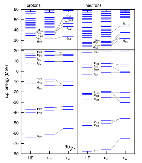
Figure 1: (Color online) The Hartree-Fock eigenenergies, the eigenenergies $e_{\alpha}$ of the new s.p. Hamiltonian and the pick-up and removal centroid energies $\pm\varepsilon_{\alpha}$, Eqs. (29), (30), for the nucleus ⁹⁰Zr, evaluated using the standard parameter set (see text). The energies are not corrected for the center-of-mass energy. A thick grey line separates the particle states from the hole states.

⁹⁰Zr nucleus. The thick grey line separates the particle states from the hole states. One can observe that the spectrum of the new eigenenergies $e_{\alpha}$ is more dense than the HF one. The centroid energies $\varepsilon_{p}$ and $\varepsilon_{h}$ are even closer to each other, on average, while the Fermi gap in this case appears larger. Indeed, the lowest pickup centroid energy corresponds to the strength distribution to one or more particle eigenstates — since there is no mixing between particle and hole configurations. Therefore, its value cannot be lower than the lowest particle state’s $e_{\alpha}$. Similar arguments explain why $e_{\alpha}\geq\varepsilon_{\alpha}$ for the highest hole level and $e_{\alpha}\leq\varepsilon_{\alpha}$ for the most bound one. Let us note also that, in general, the ordering of the $\varepsilon_{\alpha}$ levels is different than for the $e_{\alpha}$ and HF ones. In total, the $ph$ energies $e_{p}-e_{h}$ are smaller than their HF counterparts which enter the RPA equations. This means that the “unperturbed spectrum” corresponding to the ERPA equations (the one obtained by setting the $B$ matrix and the last term in Eq. (19) equal to zero, and assuming that the prefactor of the first term in Eq. (19) is roughly equal to one) will be denser than the unperturbed HF spectrum. The above remarks hold for all examined nuclei.

In Fig. 2 the deviation

Figure 2: The deviation $\Delta\rho_{\alpha}=\rho_{\alpha}-\rho_{\alpha}^{(0)}$ of the occupation probabilities $\rho_{\alpha}$ from their HF values $\rho_{\alpha}^{(0)}$ is shown for the proton single-particle levels of the nuclei ⁴⁰Ca and ⁹⁰Zr. Filled circles: standard parameter set; open circles: only natural-parity states taken into account. The energies are not corrected for the center-of-mass motion.

$\Delta\rho_{\alpha}=\rho_{\alpha}-\rho_{\alpha}^{(0)}$ of the occupation probabilities $\rho_{\alpha}$ from their HF values $\rho_{\alpha}^{(0)}$ (1 for holes, 0 for particles) is shown for the proton s.p. levels of the nuclei ⁴⁰Ca and ⁹⁰Zr. The full circles correspond to the standard parameter set. In the case of the open circles, only natural-parity excitations have been taken into account. More than half the total depletion seems to be accounted for by these excitations.

In Table 1 we list the values

Table 1: The values of the mean square deviation per particle $\sigma$, Eq. (27), found when all ${J}^{\pm}$ excitations ($\sigma_{\text{NUP}}$ - standard parameter set) and only natural-parity ($\sigma_{\text{NP}}$) ones are considered. In square brackets, for ⁹⁰Zr, results obtained within a larger s.p. basis (15 shells) are shown.

	16O	40Ca	90Zr	100Sn
$\sigma_{\text{NUP}}\times 10^{3}$	3.43	2.23	1.11[1.17]	1.37
$\sigma_{\text{NP}}\times 10^{3}$	1.85	1.05	0.46[0.48]	0.57

of the mean square deviation per particle $\sigma$, Eq. (27), that we find for the four nuclei ¹⁶O, ⁴⁰Ca, ⁹⁰Zr, ¹⁰⁰Sn when all ${J}^{\pm}$ excitations ($\sigma_{\text{NUP}}$ - standard parameter set) or only natural-parity ones ($\sigma_{\text{NP}}$) are considered. (Note that no charge-exchange excitations are considered.) $\sigma$ characterizes the depletion of the Fermi sea due to correlations. In square brackets, for ⁹⁰Zr, results obtained within a larger s.p. basis (15 shells) are shown, to verify that our conclusions remain valid. The ratio $\sigma_{\text{NP}}:\sigma_{\text{NUP}}$ is roughly 50%. We notice that the values of $\sigma$ are of the order $10^{-3}$, reflecting the effect of long-range correlations. As mentioned in Sec. III.2, such $\sigma$-values are typical of models which do not take into account short-range correlations. In principle, these are dealt with by the UCOM, but a full treatment to this end has not been pursued here. Indeed, when calculating the OBDM and the occupation probabilities $\rho_{\alpha}$, we have used the uncorrelated operators $a^{\dagger}_{\alpha}a_{\alpha^{\prime}}$. For a consistent UCOM treatment, however, correlated operators $C^{\dagger}a^{\dagger}_{\alpha}a_{\alpha^{\prime}}C$ should be considered. Such calculations are not trivial and lie beyond the scope of the present work. As a relevant example where the potential of the UCOM was fully exploited in describing short-range correlations in nuclei, we mention the calculations of Ref. Neff and Feldmeier (2003), where the high-momentum tail of the s.p. momentum distribution is reproduced.

For ⁴⁰Ca and ⁹⁰Zr we can compare our present results for the depletion of the Fermi sea to the ones obtained within second-order perturbation theory (PT) and reported in Ref. Roth et al. (2006). In general the occupation probabilities of hole states are larger in the case of ERPA, especially for ⁹⁰Zr. We note that within PT more configurations are taken into account in the evaluation of ground-state correlations, namely all the values of ${J}^{\pm}$ available within the basis, including charge-exchange excitations. More importantly, the use of non-renormalized PT is known to overestimate the depletion of the Fermi sea Van Neck et al. (1992). This can explain also why for ⁹⁰Zr the particle occupation probabilities obtained within ERPA are much smaller. For ⁴⁰Ca they are larger only close to the Fermi energy. For both nuclei the ERPA values of the particle occupation probabilities drop much faster to zero as the energy increases, compared to PT. The use of the natural-orbital basis, rather than the HF one, is responsible for this behaviour; it is not a matter of RPA vs. PT — cf. the particle occupation probabilities reported in Ref. Lenske and Wambach (1990) within (S)RPA in the HF basis.

IV.2 Collective excitations

In Fig. 3

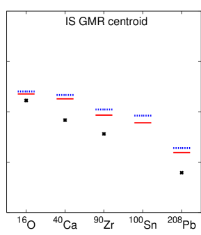
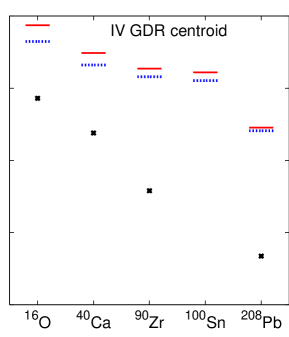
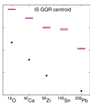
Figure 3: (Color online) Centroid energies of the IS GMR, IV GDR, and IS GQR obtained for the nuclei ¹⁶O, ⁴⁰Ca, ⁹⁰Zr, ¹⁰⁰Sn, and ²⁰⁸Pb within the RPA (red solid bars) and ERPA (blue dotted bars), compared with experimental data (black points — for references see text). The standard parameter set was used, except for ²⁰⁸Pb, where $J_{\max}=3$ and a s.p. basis of 15 shells were employed. In calculating the centroids, the strength up to 50 MeV was taken into account.

we show the centroid energies of the IS GMR, IV GDR, and IS GQR obtained for the nuclei ¹⁶O, ⁴⁰Ca, ⁹⁰Zr, ¹⁰⁰Sn, and ²⁰⁸Pb within the RPA (solid bars) and ERPA (dotted bars), compared with some experimental data (points). In Fig. 4

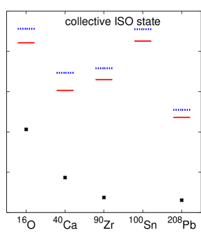
Figure 4: (Color online) As in Fig. 3, energy of the low-lying IS octupole (ISO) state.

we show the energy of the low-lying IS octupole (ISO) state. As examples, we show in Figs. 5

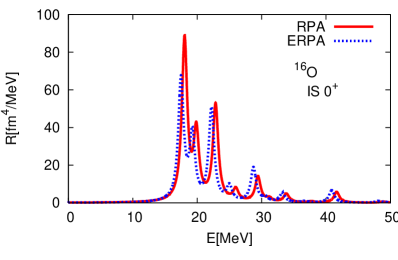
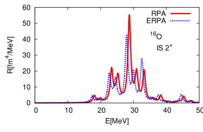
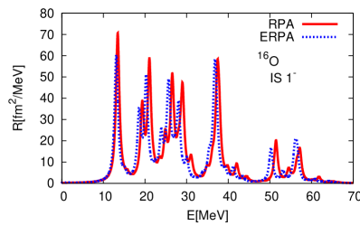
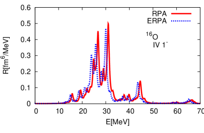
Figure 5: (Color online) IS monopole, IS quadrupole, and IS and IV dipole strength distributions of ¹⁶O computed within RPA (red solid lines) and ERPA (blue dotted lines). The discrete strength distributions have been folded with a Lorentzian of width $\Gamma=2$ MeV. The standard parameter set was used.

and 6

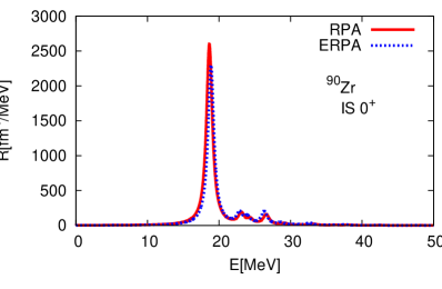
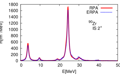
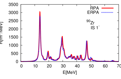
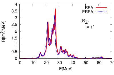
Figure 6: (Color online) As in Fig. 5, for ⁹⁰Zr.

the corresponding IS monopole, IV dipole, and IS quadrupole strength distributions for ¹⁶O and ⁹⁰Zr. Also shown in these figures are the IS dipole strength distributions. In all cases shown in Figs. 3 – 6 the standard parameter set was used, except for ²⁰⁸Pb, where a basis of 15 shells was employed to ensure better convergence in this heavy nucleus and $J_{\max}=3$ was used to avoid an extremely time-consuming calculation. The strength distributions up to 50 MeV were taken into account when calculating the centroid energies, which are defined as the first energy moment of the distribution, $m_{1}$, divided by the total strength, $m_{0}$. The experimental centroids of the IS GMR and the IS GQR were taken from Refs. Lui et al. (2001) (¹⁶O), Youngblood et al. (2001) (⁴⁰Ca), Youngblood et al. (2004a) (⁹⁰Zr), and Youngblood et al. (2004b) (²⁰⁸Pb). Photoabsorption cross sections were found in Refs. LeBrun et al. (1987) (¹⁶O), Veyssière et al. (1974) (⁴⁰Ca), Berman et al. (1967) (⁹⁰Zr), and Veyssière et al. (1970); Berman and Fultz (1975) (²⁰⁸Pb) and the centroids $m_{1}/m_{0}$ of the corresponding IV GDR strength distributions were evaluated from those. Experimental energies of the collective octupole state were adopted from Ref. Kibédi and Spear (2002).

From Fig. 3 it is evident that the energy of the GDR drops when ground-state correlations are explicitly considered within the ERPA, but not enough to reach the experimental data. In general, a decrease of no more than 1 MeV was achieved for the heavier nuclei. The same holds for the IV $0^{+}$ and $2^{+}$ centroids (not shown). The IS giant resonances, namely the IS GMR, GDR, and GQR, were less affected. In most cases, their energies were higher when evaluated within ERPA than within RPA. Apparently, in the IS case the weakening of the (attractive) residual interaction due to the depleted Fermi sea compensates for the compression of the s.p. spectra.

The energy of the collective IS octupole state, Fig. 4, increases by up to 1 MeV and the disagreement with the experimental data is worsened. We found that its strength within ERPA decreases with respect to RPA by 10-20%. Still, the ERPA values of the strength are larger than the experimental ones by a factor 1.6-2.2 for the nuclei considered. The energy of the low-lying IS quadrupole state for the nuclei ⁹⁰Zr, ¹⁰⁰Sn, and ²⁰⁸Pb (not shown) increases due to the correlations by no more than 0.3 MeV and its strength decreases by 10-20%.

We found that, for all nuclei and excitation fields examined, the total strength $m_{0}$ and total energy-weighted strength $m_{1}$ decrease within ERPA. The relative change remains below 10% in almost all cases, being largest for the lightest nuclei. Within ERPA the spurious dipole state is found at approximately 1 MeV, i.e., somewhat further from zero than within RPA.

In Fig. 7

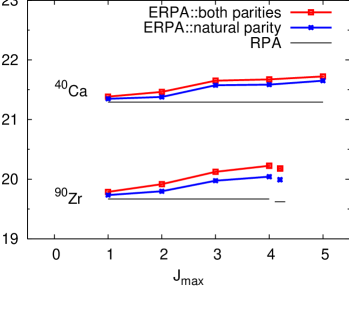
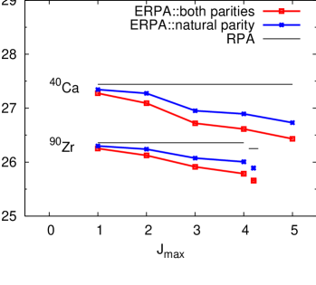
Figure 7: (Color online) The cumulative effect of allowing zero-point fluctuations of larger multipolarity $J_{\max}$ on the IS GMR and IV GDR centroids of ⁴⁰Ca and ⁹⁰Zr. Blue crosses: using only natural-parity states. Red squares: both natural- and unnatural-parity states were used. A s.p. basis of 13 shells was used. Lines are drawn to guide the eye. The horizontal lines show the RPA results for comparison. For ⁹⁰Zr and $J_{\max}=4$ an extra set of data is shown in each panel, detached from the lines. These were obtained using a larger s.p. basis of 15 shells.

we show, for ⁴⁰Ca and ⁹⁰Zr, the cumulative effect on the IS GMR and IV GDR centroids of allowing zero-point fluctuations of ever larger multipolarity $J_{\max}$. The crosses mark results obtained using only natural-parity states. The squares mark results obtained using both natural- and unnatural-parity states. Lines are drawn to guide the eye. The horizontal lines show the RPA results for comparison. In calculating the centroids, the corresponding strength distributions up to 50 MeV were taken into account. For ⁹⁰Zr and $J_{\max}=4$ an extra set of data is shown in each panel, detached from the lines. These were obtained using a larger s.p. basis of 15 shells and verify that our calculations have converged to a rather satisfactory degree with respect to the basis.

In all cases a steeper change is observed between $J_{\max}=2$ and $3$, indicating the important effect of the low-lying collective $3^{-}$ state. We see also that the convergence of our results as $J_{\max}$ increases is rather slow. As RPA calculations of ground-state energies suggest Barbieri et al. (2006), in order to achieve good convergence when describing RPA correlations one may need to take into account $J_{\max}$ values up to approximately 10. For ERPA, such large values are beyond our computational capabilities at present. Since, however, no strongly collective states with multipolarities larger than 4 are expected, and based also on the results of Ref. Barbieri et al. (2006), it is reasonable to speculate that the difference between the RPA and ERPA results would be no more than doubled if higher values of $J_{\max}$ were considered. Of course, no charge-exchange excitations have been taken into account here. These can introduce additional correlations of non-negligible amplitude, albeit smaller than the non-exchange ones Barbieri et al. (2006).

V Summary and perspectives

A correlated realistic interaction, derived from the Argonne V18 nucleon-nucleon interaction in the UCOM framework, was employed in calculations within the so-called Extended RPA (ERPA). The aim was to investigate to which extent such an interaction can describe nuclear collective motion in the framework of first-order RPA. Renormalized formulations of the RPA, such as the ERPA, consider explicitly the depletion of the Fermi sea in the ground state due to RPA correlations. In a previous work we used the same interaction within a RPA model Paar et al. (2006), where excitations are built on top of the uncorrelated HF ground state. The ERPA employed here allowed us to examine the effect of ground-state correlations on the excitation spectra. It was found that the effect on the properties of giant resonances is rather small. Compared to the standard RPA model, their centroid energies decrease by up to 1 MeV in the isovector channel. The isoscalar response is less affected in general. Ground-state properties obtained within the ERPA were compared with corresponding HF and perturbation-theory results and discussed as well.

Our results with the correlated Argonne V18 show that the RPA based on the uncorrelated HF ground state is a fairly good approximation to the actual RPA problem in the case of giant resonances, although with this interaction the HF solution is a bad approximation to the RPA ground state when one considers the nuclear binding energies. It should be noted that a theoretical error of 1 MeV in the centroid energies (or more, if charge-exchange and higher-mutipole correlations are included) can be important in certain applications. That said, the inability of our (E)RPA calculations to reproduce the experimental data should originate elsewhere. Up to now we have assumed that residual three-body forces can be neglected, based upon the fact that they contribute only marginally to the ground-state energy as calculated within many-body perturbation theory Roth et al. (2005). This is not necessarily a valid assumption. We are currently constructing a simple phenomenological zero-range three-body force, to be used along with the correlated two-nucleon interaction in future calculations. Preliminary results show that by using such a three-body force it is possible to improve on the description of observables such as nuclear radii and resonance energies while retaining the good reproduction of the experimental binding energies.

Another important issue is that, within the RPA, one neglects the coupling to higher-order configurations ($2p2h$ and beyond). Collective excitations can be significantly affected by the inclusion of $2p2h$ configurations, as preliminary SRPA results show. Therefore, SRPA calculations will also be the subject of future work. In principle, it is possible to combine the SRPA with a correlated ground state Dro$\dot{\mathrm{z}}$d$\dot{\mathrm{z}}$ et al. (1990); Gambacurta et al. (2006) for a most complete theoretical treatment of nuclear excitations.