Abstract

A semi-microscopic self-consistent quantum approach developed recently to describe the inner crust structure of neutron stars within the Wigner-Seitz (WS) method with the explicit inclusion of neutron and proton pairing correlations is further developed. In this approach, the generalized energy functional is used which contains the anomalous term describing the pairing. It is constructed by matching the realistic phenomenological functional by Fayans et al. for describing the nuclear-type cluster in the center of the WS cell with the one calculated microscopically for neutron matter. Previously the anomalous part of the latter was calculated within the BCS approximation. In this work corrections to the BCS theory which are known from the many-body theory of pairing in neutron matter are included into the energy functional in an approximate way. These modifications have a sizable influence on the equilibrium configuration of the inner crust, i.e. on the proton charge $Z$ and the radius $R_{c}$ of the WS cell. The effects are quite significant in the region where the neutron pairing gap is larger.

PACS. 26.60.+c Nuclear matter aspects of neutron stars – 97.60.Jd Neutron stars – 21.65.+f Nuclear matter – 21.60.-n Nuclear structure models and methods – 21.30.Fe Forces in hadronic systems and effective interactions

1 Introduction

Recently, we have developed a semi-microscopic self-consistent approach to describe the neutron star inner crust with the explicit inclusion of neutron and proton pairing correlations [1, 2]. The inner crust is the part of the neutron star shell with subnuclear densities, $0.001\rho_{0}\leq\rho\leq 0.5\rho_{0}$, where $\rho_{0}$ is the normal nuclear density. It is a crystal system consisting mainly of spherically symmetrical nuclear-like clusters immersed in a sea of neutrons and virtually uniform sea of electrons. The quantum self-consistent description of the inner crust goes back to the classical paper by Negele and Vautherin (N&V)[3] who used a kind of energy functional method combined with the Wigner-Seitz (WS) method to describe the crystal structure effects in an approximate way. Within this approach, for a fixed average nuclear density $\rho$, the energy functional of the system is minimized for the spherical WS cell of the radius $R_{c}$. A cell contains $A=(4\pi/3)R_{c}^{3}\rho$ nucleons, specifically $Z$ protons and $N=A-Z$ neutrons. As far as the system is electro-neutral, the number of electrons per a cell is equal to $Z$. For a mature neutron star which can be considered at zero temperature and neutrino free, the $\beta$-stability condition consists in equality of the neutron chemical potential $\mu_{n}$ to the sum of the proton and electron ones, $\mu_{p}{+}\mu_{e}$. For a wide region of $\rho$, the minimization procedure was carried out in [3] for different values of $Z$ and $R_{c}$ resulting in the equilibrium configuration ($Z,R_{c}$) for the density under consideration.

It should be noted that the pairing effects were not taken into account in [3]. Thus, the approach developed in [1, 2] could be considered as a generalization of the N&V method with allowance for pairing effects. Although the contribution of the pairing to the total binding energy of the system under consideration is rather small, it turned out that it may to change the equilibrium configuration ($Z,R_{c}$) significantly.

To involve the pairing effects in a self-consistent way, we use the generalized energy functional method [4] which incorporates in a natural way the pairing into the original Kohn-Sham [5] method. In this approach, the interaction part of the generalized energy functional is the sum of the normal component, ${\cal E}_{\rm norm}(\rho)$, and the anomalous one, ${\cal E}_{\rm an}(\rho,\nu)$. They depend on the normal densities ($\rho_{n},\rho_{p}$) and the anomalous ones, ($\nu_{n},\nu_{p}$). Just as in the Kohn-Sham method, the prescription $m^{*}=m$ holds to be true. The so-called Superfluid LDA method suggested recently [6] is rather close to the method by S. Fayans et al. The main difference between the two approaches is in the form of the density dependence of the anomalous term of the energy functional.

In [1, 2] the semi-microscopic energy functional was constructed with matching at the nuclear cluster surface the phenomenological nuclear functional ${\cal E}^{\rm ph}$ by Fayans et al. [4] inside the cluster to a microscopic one, ${\cal E}^{\rm mi}$, for the neutron environment. The normal part of ${\cal E}^{\rm mi}$ was found in [7] within the Brueckner approach with the Argonne v₁₈ potential [8] . The anomalous component of ${\cal E}^{\rm mi}$ was calculated in [1, 2] within the Bardeen-Cooper-Schrieffer (BCS) approximation for neutron matter, again with the use of the v₁₈ potential.

It is well known that the BCS approximation overestimates the gap value $\Delta_{n}$ in neutron matter. Various many-body corrections suppress the value of $\Delta_{n}^{\rm BCS}$ significantly. Although up to now there is no consistent many-body theory of pairing in neutron matter, there exists a conventional point of view (see e.g. [9]) that the BCS gap value is suppressed,

$$\Delta_{n}(k,k_{\mbox{\scriptsize F}})=f_{\rm m-b}(k,k_{\mbox{\scriptsize F}})\Delta_{n}^{\rm BCS}(k,k_{\mbox{\scriptsize F}}),$$ (1)

by a factor $f_{\rm m-b}(k,k_{\mbox{\scriptsize F}})$ which is between 1/2 and 1/3. The only exception seems to be the work in ref. [10]. In this paper, we use a simple model for the many-body corrections in which the suppression factor $f_{\rm m-b}(k,k_{\mbox{\scriptsize F}})$ is supposed to be momentum and density independent. This ansatz is essentially similar to that used in [11] for considering the structure of a superfluid vortex in neutron matter. We modify the anomalous component of the energy functional of [1, 2] by introducing the constant suppression factor. We examine two versions of this model, the P2 model ($f_{\rm m-b}=1/2$) and the P3 one ($f_{\rm m-b}=1/3$). In this notation, it is natural to name the BCS approximation ($f_{\rm m-b}=1$) as the P1 model. We expect that the real truth is somewhere between the P2 and P3 models.

One more remark should be made before going to the body of the article. As it was found recently [12], there are internal uncertainties inherent to the WS method applied to the neutron star inner crust. They originate from the kind of the boundary conditions for the single-particle functions used in the WS method. There are two kinds of such boundary conditions which a priori seem equivalent. As it turned out, the corresponding predictions for the equilibrium configurations ($Z,R_{c}$) are in general different. As a rule, the difference is not large, corresponding to variation of $Z$ by 2 – 6 units and of $R_{c}$, by 1 – 2 fm. However, sometimes strong changes in the neutron single-particle spectrum arise which influence the solution of the gap equation significantly. Therefore, for each model under consideration, we carried out calculations for both kinds of boundary conditions.

2 Modification of the BCS anomalous part of the Generalized Energy Functional

The ansatz of [1, 2] for the complete energy functional consists in a smooth matching of the phenomenological and the microscopic functionals at the cluster surface:

$${\cal E}(\rho_{\tau}({\bf r}),\nu_{\tau}({\bf r}))={\cal E}^{\rm ph}(\rho_{\tau}({\bf r}),\nu_{\tau}({\bf r}))+\left({\cal E}^{\rm mi}(\rho_{\tau}({\bf r}),\nu_{\tau}({\bf r}))-{\cal E}^{\rm ph}(\rho_{\tau}({\bf r}),\nu_{\tau}({\bf r}))\right)\left(1-F_{m}(r)\right),$$ (2)

where $\tau=n,p$ is the isotopic index and the matching function $F_{m}(r)$ is a two-parameter Fermi function. The latter is taken to be the same for the normal and the anomalous components of the energy functional, with the diffuseness parameter $d_{m}{=}0.3\;$fm and the matching radius $R_{m}$ which should be chosen anew in any new case, in accordance with the equality of $\rho_{p}(R_{m})=0.1\rho_{p}(0)$. For such a choice, practically all the protons are located inside the radius $R_{m}$. Therefore, the matching procedure concerns,in fact, only neutrons, protons being described with the pure phenomenological nuclear energy functional. In practice, we use in Eq. (2) an approximation in which only neutron components of the microscopic and phenomenological functionals are taken into account in the second term containing the difference of (${\cal E}^{\rm mi}-{\cal E}^{\rm ph}$).

Following to [1, 2], we use for the microscopic part of the normal component of the total energy functional (2) the one calculated in [7] for neutron matter with the Argonne v₁₈ potential. Its explicit form could be found in the cited articles. Here we concentrate on the anomalous part of the energy functional which will be modified in comparison with that of [1, 2].

The anomalous part of the energy functional used in [1, 2] has the form:

$${\cal E}_{\rm an}=\frac{1}{2}\sum_{\tau}{\cal V}_{{\rm an},\tau}^{\rm eff}(r)|\nu_{\tau}({\bf r})|^{2},$$ (3)

where ${\cal V}_{{\rm an},\tau}^{\rm eff}$ is the density dependent effective pairing interaction.

The matching relation (2) for the anomalous part of the energy functional leads to the analogous relation for the effective pairing interaction:

$${\cal V}_{\rm an}^{\rm eff}(r)={\cal V}_{\rm eff}^{\rm ph}(\rho(r))F_{m}(r)+{\cal V}_{\rm eff}^{\rm mi}(\rho(r))(1-F_{m}(r)).$$ (4)

The isotopic index $\tau$ is for brevity omitted.

We shall use the same phenomenological effective pairing interaction ${\cal V}_{\rm eff}^{\rm ph}$ as in [1, 2], therefore we omit here its explicit form. Let us note only that it has a density dependent coordinate delta-function form of [4]. The explicit form of the density dependence [4] was modified a little in [1] in accordance with (4). As to the microscopic effective pairing interaction, it was calculated in [1] microscopically within the BCS approximation with the same Argonne force v₁₈ as the normal part of the energy functional . In this paper, we modify this procedure to take into account approximately the many-body corrections to the BCS approximation. Let us first repeat the BCS procedure.

The microscopic part of the effective pairing interaction, ${\cal V}_{\rm eff}^{\rm mi}(r)$, should be found for the model space $S_{0}$ under consideration which is limited with the energy $E_{0}$ for the single-particle spectrum. For a fixed value of the neutron density $\rho_{n}(r)$, it is defined via the gap equation in homogeneous neutron matter with the density $\rho=\rho_{n}(r)$. We start from the BCS approximation in which the gap $\Delta$ is expressed directly in terms of the bare NN potential $v(k,k^{\prime})$ in the $1S_{0}$ channel:

$$\Delta(k)\,=\,-\sum_{k^{\prime}}v(k,k^{\prime})\frac{\Delta(k^{\prime})}{2E(k^{\prime})},$$ (5)

where $E(k)=\sqrt{(\varepsilon_{k}-\mu_{n})^{2}+\Delta^{2}(k)}$, $\varepsilon_{k}=k^{2}/2m+U_{n}$, $U_{n}$ is the value of the neutron matter potential well. In terms of the effective pairing interaction, the gap equation looks analogously, but the integration in the momentum space is limited within the model space $S_{0}$:

$$\Delta(k)\,=\,-\sum_{k^{\prime}<k_{0}}{\cal V}_{\rm eff}^{\rm mi}(k,k^{\prime})\frac{\Delta(k^{\prime})}{2E(k^{\prime})},$$ (6)

where $k_{0}=\sqrt{2m(E_{0}+\mu_{n}-U_{n})}$.

In the BCS approximation the relation between the effective pairing interaction and the bare NN potential is obvious:

$${\cal V}_{\rm eff}^{\rm mi}(k,k^{\prime})\,=\,v(k,k^{\prime})-\sum_{k_{1}>k_{0}}v(k,k_{1})\frac{1}{2E(k_{1})}{\cal V}_{\rm eff}^{\rm mi}(k_{1},k^{\prime}).$$ (7)

The effective pairing interaction entering Eq.(6) depends explicitly on momenta, which corresponds to a non-local force in the coordinate space. In view of very simple local form of the phenomenological effective pairing interaction ${\cal V}_{\rm eff}^{\rm ph}$ in Eq. (4), for matching it is necessary to simplify the microscopic partner ${\cal V}_{\rm eff}^{\rm mi}$ to a local form, too. The simplest way is, for a fixed value of $\rho$ under consideration, to define it as a $k$-independent average value of the effective pairing interaction in Eq. (6) which yields the same value $\Delta(k_{\mbox{\scriptsize F}})$ as the exact effective pairing interaction:

$$\Delta(k_{\mbox{\scriptsize F}})\,=\,-\bar{{\cal V}}_{\rm eff}^{\rm mi}(k_{\mbox{\scriptsize F}})\sum_{k^{\prime}<k_{0}}\frac{\Delta(k^{\prime})}{2E_{0}(k^{\prime})},$$ (8)

where $k_{\mbox{\scriptsize F}}$ is the local Fermi momentum $k_{\mbox{\scriptsize F}}=(3\pi^{2}\rho)^{1/3}$, and $E_{0}(k)=\sqrt{(\varepsilon_{k}-\mu_{n})^{2}+\Delta^{2}(k_{\mbox{\scriptsize F}})}$. For the Fermi momentum $k_{\mbox{\scriptsize F}}$ under consideration, the microscopically calculated value of $\Delta(k_{\mbox{\scriptsize F}})$ is the only input of Eq. (8) to find the effective pairing interaction $\bar{{\cal V}}_{\rm eff}^{\rm mi}(k_{\mbox{\scriptsize F}})$. In the BCS (or P1) model, one uses $\Delta^{\rm BCS}(k_{\mbox{\scriptsize F}})$ in Eq. (8). In the P2 or P3 models the value of $\Delta(k_{\mbox{\scriptsize F}})$ is found from Eq. (1) with $f_{\rm m-b}{=}1/2$ or 1/3, correspondingly. Then it should be substituted into Eq. (8). The resulting values of the effective pairing interaction in neutron matter for the case of the P1 (BCS), P2 and P3 models are displayed in Fig. 1.

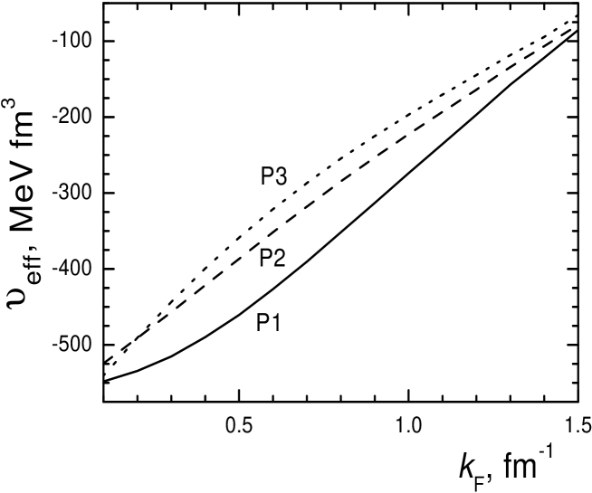
Figure 1: The effective pairing interaction in neutron matter for the P1 , P2 and P3 models (solid, dashed and dotted line, correspondingly).

Let us now discuss the problem of the boundary conditions in the WS method mentioned above. For the case of the BCS approximation, it was examined in [12]. Application of the variational principle to the energy functional under consideration for a WS cell results in the set of the Shrödinger-type equations for the single particle neutron functions $\phi_{\lambda}({\bf r})=R_{nlj}(r)\Phi_{ljm}({\bf n})$, with the standard notation. The radial functions $R_{nlj}(r)$ obey the boundary conditions at the point $r=R_{c}$. There exist different kinds of the boundary conditions. N&V used the following one:

$$R_{nlj}(r=R_{c})=0$$ (9)

for odd $l$, and

$$R^{\prime}_{nlj}(r=R_{c})=0,$$ (10)

for even ones. In [12] it was denoted as BC1. An alternative kind of the boundary conditions (BC2) was considered also there, when Eq. (9) is valid for even $l$ whereas Eq. (10), for odd ones. As the analysis of [12] for the BCS case (P1 model) has shown, some predictions of the two versions of the boundary conditions (BC1 versus BC2) are in general different. In this paper, we will perform the similar analysis for the P2 and P3 models.

3 A brief summary of the pairing effects in the case of the BCS approximation

Calculations of [1, 2] were carried with the use of the BCS approximation for the neutron matter pairing and the N&V version of the boundary conditions (BC1, in our notation). As it turned out, the pairing correlations influence the equilibrium values of ($Z,R_{c}$) significantly. In the paper [12], for the case of the BCS approximation (i.e., the P1 model), the dependence of the ground state properties of the inner crust on the kind of the WS boundary conditions was examined. The calculations were carried out directly with the two kinds of boundary conditions, BC1 and BC2, and the results were compared with each other. To make the analogous analysis for the P2 and P3 models in the next sections more transparent, we cite here some results of [12]. In particular, Fig. 2 shows the values of the binding energy per a nucleon, $E_{\rm B}$, for the P1 model calculated with the two versions of the boundary conditions.

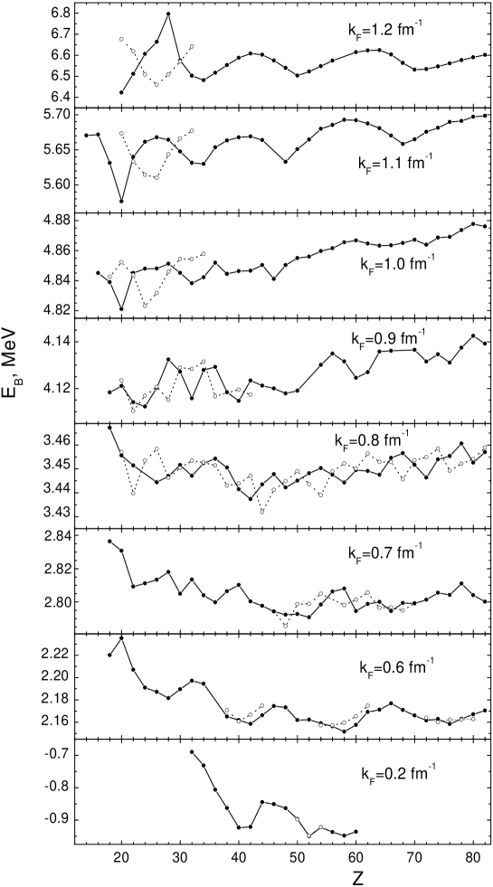
Figure 2: Binding energy per a nucleon for various $k_{\mbox{\scriptsize F}}$ in the BC1 case (solid circles connected with the solid lines) and the BC2 one (open circles connected with the dotted lines).

We see that in the case of very small density, $k_{\mbox{\scriptsize F}}{=}0.2\;$fm^-1, which is nearby the neutron drip point, the predictions of the BC1 and BC2 versions are practically identical. At increasing density, with $k_{\mbox{\scriptsize F}}\geq 0.6\;$fm^-1, the uncertainty in the equilibrium value of $Z$ is between 2 and 6 units, with the largest values at the largest $k_{\mbox{\scriptsize F}}$. The uncertainty in the value of $R_{c}$ is, as a rule, about 1 fm and only for $k_{\mbox{\scriptsize F}}{=}1.1\;$fm^-1 it turns out to be about 2 fm. Referring to [2, 12] for more details, we present in Table 1 the main ground state characteristics of the inner crust. There are two lines for each value of $k_{\mbox{\scriptsize F}}$. The first one is given for the $Z$ value corresponding to the minimum of the binding energy $E_{\rm B}$ in the BC1 case, the second one, for BC2. The only exception is $k_{\mbox{\scriptsize F}}{=}0.2\;$fm^-1 where these two values of $Z$ coincide. It should be stressed that, as a rule, the value of these uncertainties is smaller than the variations of the equilibrium configuration ($Z,R_{c}$) connected with the pairing effects [2]. One more point which is important for the analogous consideration within the P2 and P3 models is as follows. For all the values of $k_{\mbox{\scriptsize F}}$ which were investigated, the relative position of the local minima of the functions $E_{\rm B}(Z)$ is always similar for the BC1 case and the BC2 one. As the result, the corresponding absolute minima are rather close to each other.

Table 1: Comparison of characteristics of equilibrium configurations of the WS cell for two different kinds of the boundary conditions in the case of the P1 model (BCS approximation).

$k_{\rm F},$	$\,Z\,$	$R_{\rm c},\;$fm		$E_{\rm B},\;$MeV		$\mu_{n},\;$MeV
${\rm fm^{-1}}$		BC1	BC2	BC1	BC2	BC1	BC2
0.2	52	57.18	57.10	-0.9501	-0.9483	0.1928	0.1942
0.6	58	37.51	37.48	2.1516	2.1596	3.2074	3.2226
	56	36.97	36.95	2.1563	2.1572	3.2173	3.2193
0.7	52	32.02	32.04	2.7908	2.7989	3.9876	4.0107
	48	31.16	31.14	2.7924	2.7856	4.0069	3.9873
0.8	42	26.90	26.91	3.4373	3.4471	4.8454	4.8561
	44	27.29	27.30	3.4435	3.4319	4.8553	4.8198
0.9	24	20.26	20.30	4.1123	4.1169	5.7340	5.7986
	22	19.87	19.70	4.1141	4.1104	5.7861	5.7170
1.0	20	16.69	16.90	4.8210	4.8522	6.8525	6.7424
	24	18.29	18.22	4.8479	4.8231	6.8446	6.8920
1.1	20	14.99	15.33	5.5765	5.6733	7.4288	8.0446
	26	16.75	17.08	5.6677	5.6100	7.9680	8.5398
1.2	20	13.68	13.95	6.4225	6.6762	8.5814	9.1898
	26	15.21	14.89	6.6639	6.4587	9.0825	9.3413

Table 2 collects some important characteristics of the gap for all the density values under consideration. The relative position of two lines for the same value of $k_{\mbox{\scriptsize F}}$ is the same as in Table 1, i.e. the first line corresponds to Z from the equilibrium ($Z,R_{c}$) configuration for the BC1 version. The following notation is used. The asymptotic value of the Fermi momentum $k_{\rm F}^{\rm as}$ corresponds to the asymptotic value of the density $\rho(r)$ averaged over the interval $R_{c}{-}b<r<R_{c}$, $b{=}2\;$fm. The asymptotic gap value $\Delta_{\rm as}$ is found as the average of $\Delta(r)$ over the same interval. The central gap value $\Delta(0)$ is calculated as the average of $\Delta(r)$ over the interval $0<r<3\;$fm. The Fermi average gap $\Delta_{\mbox{\scriptsize F}}$ is defined as the average value of the diagonal matrix element of the neutron gap at the Fermi surface. The averaging procedure involves 10 levels above $\mu_{n}$ and 10 levels below. At last, $\Delta_{\rm inf}$ means the infinite neutron matter gap value found within the BCS approximation for the density $\rho$ corresponding to the Fermi momentum $k_{\rm F}^{\rm as}$, and $\Delta^{0}_{\rm inf}$ is the same for the Fermi momentum $k_{\rm F}$. Let us remind that the latter corresponds to the average nucleon density under consideration. Obviously, the inequality $k_{\rm F}^{\rm as}<k_{\rm F}$ takes place because the WS cell contains a nuclear-like cluster in the center with the density which exceeds the average one. The difference is especially large in the case of $k_{\rm F}{=}0.2\;$fm which is nearby the neutron drip point. Indeed, in this case almost all the matter is concentrated in the central blob. So big difference between the values of $\Delta_{\rm inf}$ and $\Delta^{0}_{\rm inf}$ for $k_{\rm F}{=}0.2\;$fm is explained, first, by the big difference between two values of the Fermi momentum and, second, with the sharp dependence of the $\Delta_{n}$ in neutron matter on $k_{\mbox{\scriptsize F}}$ at small $k_{\mbox{\scriptsize F}}$.

It is worth to mention that the difference between the asymptotic $\Delta_{\rm as}$ value and the infinite neutron matter prediction $\Delta_{\rm inf}$ is a measure of validity of the LDA for the gap calculation outside the central nuclear cluster. One can see that, as a rule, the LDA works within 10% accuracy, but sometimes the difference is greater which is an evidence of the so-called proximity effect. The Fermi average value $\Delta_{\mbox{\scriptsize F}}$ is usually very close to $\Delta_{\rm as}$ value. It is explained with the fact that the region out of the nuclear cluster, in which the function $\Delta(r)$ is almost a constant, contributes mainly to the matrix elements of $\Delta$ nearby the Fermi surface.

Table 2: Average gap characteristics in the P1 model (BCS approximation).

$k_{\rm F},\!\!$	$Z$	$k_{\rm F}^{\rm as},\,{\rm fm^{-1}}$		$\Delta(0),\;$MeV		$\Delta_{\rm as},\;$MeV		$\Delta_{\rm F},\;$MeV		$\Delta_{\rm inf},\;$MeV		$\Delta^{0}_{\rm inf},\!\!$
$\rm fm^{-1}\!\!$		BC1	BC2	BC1	BC2	BC1	BC2	BC1	BC2	BC1	BC2	MeV
0.2	52	0.1156	0.1095	0.088	0.132	0.042	0.046	0.043	0.058	0.126	0.106	0.40
0.6	58	0.5786	0.5783	1.464	1.471	1.947	1.899	1.919	1.893	2.321	2.320	2.42
	56	0.5783	0.5786	1.456	1.428	1.899	1.912	1.893	1.891	2.319	2.321
0.7	52	0.6758	0.6753	1.665	1.650	2.358	2.288	2.300	2.247	2.680	2.678	2.76
	48	0.6763	0.6763	1.679	1.648	2.312	2.368	2.290	2.325	2.682	2.682
0.8	42	0.7732	0.7724	1.767	1.726	2.614	2.546	2.555	2.445	2.883	2.882	2.93
	44	0.7729	0.7727	1.747	1.834	2.580	2.679	2.525	2.560	2.883	2.883
0.9	24	0.8694	0.8693	1.862	1.664	2.777	2.625	2.636	2.506	2.919	2.919	2.92
	22	0.8725	0.8664	1.936	1.654	2.677	2.680	2.617	2.544	2.918	2.919
1.0	20	0.9499	0.9613	1.249	1.966	2.199	2.635	2.023	2.517	2.800	2.773	2.68
	24	0.9612‘	0.9574	1.894	1.504	2.705	2.507	2.519	2.288	2.774	2.782
1.1	20	1.0315	1.0531	0.996	1.889	1.477	2.411	1.318	2.317	2.550	2.458	2.26
	26	1.0434	1.0649	1.927	1.296	2.469	2.242	2.280	2.020	2.500	2.408
1.2	20	1.1243	1.1321	1.556	0.992	1.340	2.017	1.210	1.558	2.113	2.066	1.66
	26	1.1278	1.1160	0.760	0.991	1.549	0.963	1.249	0.862	2.092	2.163

For the case of small and intermediate densities, $k_{\mbox{\scriptsize F}}<1\;$fm^-1, the influence of a particular choice of the boundary conditions, BC1 or BC2, to the value of $\Delta_{\mbox{\scriptsize F}}$ or $\Delta_{\rm as}$ is not essential. As the result, the uncertainty in predictions for the gap function $\Delta(r)$ caused by this choice of the boundary conditions is also rather small. An example for $k_{\rm F}{=}0.8\;$fm is given in Fig. 3. The difference between any couple of these curves is less than the accuracy of the approach, and any of them could be used as a prediction for $\Delta(r)$. To be definite, let us consider the “self-consistent” gap function for the BC1 version of the boundary conditions as the prediction of the WS method for $\Delta(r)$ in the case of small and intermediate densities, $k_{\mbox{\scriptsize F}}<1.0\;$fm^-1. In the case of $k_{\mbox{\scriptsize F}}{=}0.8\;$fm^-1 under consideration it corresponds to $Z{=}42$. Such a choice is similar to that used in [2].

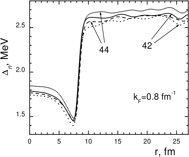
Figure 3: The neutron gap for $k_{\mbox{\scriptsize F}}{=}0.8\;$fm^-1, $Z{=}42$ and $Z{=}44$, in the BC1 case (solid lines) and in the BC2 one (dashed lines).

Fig. 4 collects predictions for $\Delta(r)$ in the BCS approximation for these values of $k_{\mbox{\scriptsize F}}$. In accordance with the above agreement, the BC1 kind of the boundary conditions is used. The value of $k_{\mbox{\scriptsize F}}{=}1\;$fm^-1 is included as an optional one as far as in this case the uncertainty is not negligible (about 20%) but it is not so big as the one for higher values of $k_{\mbox{\scriptsize F}}$.

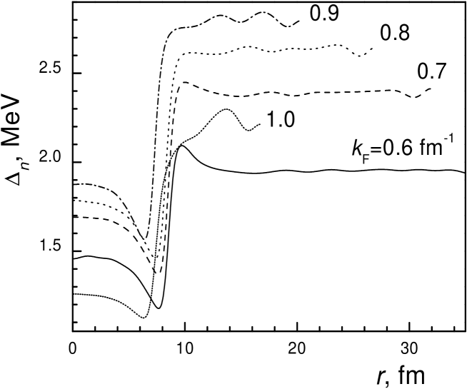
Figure 4: The gap $\Delta(r)$ for $k_{\mbox{\scriptsize F}}{=}0.6\div 1.0\;$fm^-1, the P1 (BCS) model, and the BC1 version of boundary condition.

On the contrary, as it is seen in Table 2, in the case of high densities, $k_{\mbox{\scriptsize F}}\stackrel{{\scriptstyle\scriptstyle>}}{{\phantom{}{}_{\sim}}}1\;$fm^-1, the uncertainty in the value of the neutron gap is rather large. As it was shown in [12], such big variations (BC1 versus BC2) of the gap value in the WS approximation appear due to the shell effect in the neutron single-particle spectrum which is rather pronounced in the case of high $k_{\mbox{\scriptsize F}}$ and, correspondingly, small $R_{c}$ values. We consider this effect as an artifact of the WS method which should disappear in a more consistent approach. In [12], we suggested an approximate recipe to avoid this uncertainty for the gap function $\Delta(r)$. This topic will be discussed in more detail in the next two sections where the P2 and P3 models are considered with the many-body corrections to the BCS approximation taken into account.

4 Pairing effects in the case of the P2 model

Let us go to the P2 model in which the many-body corrections to the BCS approximation are taken into account in an approximate way outlined in Section 2, with the factor $f_{\rm m-b}{=}1/2$ in Eq. (1) for the gap $\Delta(k_{\mbox{\scriptsize F}})$ which is the input for finding the effective pairing interaction from Eq. (8). The calculation scheme itself and the presentation of results are mainly similar to those for the P1 model in the previous section. In particular, again two kinds of boundary conditions, BC1 and BC2, are used, and the dependence of the results on the choice is analyzed. Fig. 5 shows the values of the binding energy per nucleon for the P2 model, to be compared to Fig. 2, where the P1 model is considered. It is not so detailed as Fig. 2 because, according to the experience within the P1 model, we limit the analysis to the vicinity of the absolute minimum of the function $E_{\rm B}(Z)$ as found for the P1 model. Let us first discuss the results with the BC1 boundary conditions. In this case, a detailed analysis was made for $k_{\mbox{\scriptsize F}}{=}0.9\;$fm^-1, $k_{\mbox{\scriptsize F}}{=}1.1\;$fm^-1 and $k_{\mbox{\scriptsize F}}{=}1.2\;$fm^-1. Comparison with Fig. 2 shows that, at a fixed value of $k_{\mbox{\scriptsize F}}$, the positions of the local minima in the P2 model are close to those in the P1 model. Besides, the relative positions of the absolute minimum and the local ones are the same for the two models. Therefore for other values of $k_{\mbox{\scriptsize F}}$ we examined only the vicinity of the corresponding absolute minimum in the P1 model. The only exception is the “suspicious” case of $k_{\mbox{\scriptsize F}}{=}0.7\;$fm^-1 for which, in the P1 model, the values of $E_{\rm B}(Z)$ in two local minima are rather close. The systematic calculation (with the step $\delta Z{=}4$, instead of the regular one, $\delta Z{=}2$) showed that in this case the general rule formulated above is also valid.

Let us consider now the results in the case of the BC2 kind of boundary conditions. Again the situation is quite similar to that in the P1 model, as confirmed by the detailed comparison of the two sets of calculations for the BC1 and BC2 versions in the case of $k_{\mbox{\scriptsize F}}{=}0.9\;$fm^-1. Therefore, just as in the P1 model, in the case of the BC2 boundary conditions one can limit the analysis in the vicinity of the absolute minimum for the BC1 one.

Table 3 presents the main ground state characteristics of the neutron star inner crust within the P2 model. It is organized similarly to Table 1. One can see that for all the values of $k_{\mbox{\scriptsize F}}$ under consideration, with the exception of $k_{\mbox{\scriptsize F}}{=}0.8\;$fm^-1, the equilibrium values of $Z$ in the BC1 and BC2 cases are different. Let us now compare the equilibrium $Z$ values in the P2 model with those in the P1 model (Table 1) for the BC1 case. One can see that at high densities, $k_{\mbox{\scriptsize F}}\geq 1.0\;$fm^-1, they coincide, being equal to $Z{=}20$. The maximal difference, $\delta Z{=}Z^{(\rm P1)}{-}Z^{(\rm P2)}{=}6$, occurs in the case of $k_{\mbox{\scriptsize F}}{=}0.7\;$fm^-1. It can be explained with the very flat dependence of $E_{\rm B}$ on $Z$ in this case. Therefore any change of the calculation parameters, namely, of the gap value in neutron matter $\Delta_{n}$ in the P2 model versus the P1 one, can shift the position of the minimum significantly. The difference of the WS cell radius values, $\delta R_{c}{=}R_{c}^{(\rm P1)}{-}R_{c}^{(\rm P2)}$, at a given $k_{\mbox{\scriptsize F}}$ appears mainly due to the difference in $\delta Z$. It is usually of the order of 1 fm, and only in the same case of $k_{\mbox{\scriptsize F}}{=}0.7\;$fm^-1 $\delta R_{c}$ exceeds 2 fm. Let us now analyze the influence of the kind of boundary conditions on the ground state characteristics in the case of the P2 model. In general, this effect is of the same magnitude as in the P1 model. Again the uncertainty in the equilibrium value of $Z$ is between 2 and 6 units and in the value of $R_{c}$, about $1-2\;$fm. A more detailed comparison with Table 1 shows that, as a rule, the effect of the boundary conditions in the P2 model is less than that in the P1 one, but only a little. For example, at $k_{\mbox{\scriptsize F}}{=}0.8\;$fm^-1 the equilibrium Z values for the BC1 and BC2 cases are now equal to each other. However, there is the case of $k_{\mbox{\scriptsize F}}{=}0.9\;$fm^-1 in which the effect under discussion is stronger in the P2 model. It should be noted that in the case of $k_{\mbox{\scriptsize F}}{=}1.2\;$fm^-1 the first line of the table ($Z{=}20$) contains empty positions corresponding to the BC2 version. This means that in the case under consideration (the P2 model, the BC2 type of boundary conditions and $Z{=}20$) the WS solution of the type we consider, i.e. the WS cell with a nuclear type cluster in the center, is not stable. This is a signal of proximity to the point of instability for the phase transition to the homogeneous state. In fact, for such high density values corresponding to $k_{\mbox{\scriptsize F}}{=}1.2\;$fm^-1 [14, 13] and, maybe, to $k_{\mbox{\scriptsize F}}{=}1.1\;$fm^-1 [14] the so-called “spaguetti” phase should appear which can not be described within the WS method with the spherical symmetry assumed. Therefore our consideration of these $k_{\mbox{\scriptsize F}}$ should be considered as optional, and the corresponding results are reported mainly for methodological reason.

Table 3: Comparison of characteristics of equilibrium configurations of the WS cell for two different kinds of the boundary conditions in the case of the P2 model.

$k_{\rm F,}$	$\,\,Z\,$	$R_{\rm c},\;$fm		$E_{\rm B},\;$MeV		$\mu_{\rm n},\;$MeV
${\rm fm^{-1}}$		BC1	BC2	BC1	BC2	BC1	BC2
0.6	56	36.85	36.88	2.2837	2.2842	3.4755	3.4818
	54	36.02	36.04	2.2838	2.2839	3.4660	3.4629
0.7	46	30.31	30.28	2.9320	2.9354	4.2892	4.2451
	48	30.98	30.88	2.9332	2.9348	4.3004	4.2533
0.8	40	25.97	26.19	3.5781	3.5807	5.0762	5.0987
0.9	20	18.34	18.60	4.2173	4.2452	5.7027	5.8477
	26	20.38	20.93	4.2416	4.2273	5.8894	6.0839
1.0	20	16.56	16.94	4.8641	4.9427	7.5247	6.8272
	24	18.25	17.80	4.9411	4.9013	7.0171	6.3298
1.1	20	15.05	15.42	5.5734	5.7363	9.0601	7.9905
	24	16.56	16.16	5.7339	5.6387	8.2971	6.9493
1.2	20	13.73	-	6.4175	-	8.1824	-
	26	15.30	14.90	6.9244	6.4566	8.9542	10.4879

Let us now turn to the analysis of the neutron gap. The main gap characteristics in the P2 model are collected in Table 4 which is analogous to Table 2 in the previous section. Comparison of these two tables shows that the main effect of changing from the P1 to the P2 model is quite trivial. It is a general suppression of the gap characteristics approximately by a factor two in comparison with the P1 model (i.e. within the BCS approximation). The ratio $\Delta^{(\rm P2)}/\Delta^{(\rm P1)}$ is equal to 1/2 exactly for the quantity $\Delta^{0}_{\rm inf}$ and approximately for $\Delta_{\rm inf}$. For other characteristics, the deviation of the ratio from 1/2 is usually a little greater than for $\Delta_{\rm inf}$ and only in few cases it is significant. The Fermi average value $\Delta_{\rm F}$ is the most important neutron gap characteristic. Let us compare its values for the BC1 and BC2 versions of the boundary conditions. Just as in the P1 model, the difference $\Delta_{\rm F}^{\rm BC1}{-}\Delta_{\rm F}^{\rm BC2}$ is very small for $k_{\mbox{\scriptsize F}}{=}0.6\div 0.8\;$fm^-1. For $k_{\mbox{\scriptsize F}}>0.8\;$fm^-1 the influence of the boundary conditions on the $\Delta_{\rm F}$ value becomes rather strong, significantly stronger than in the P1 model. Especially strong effect appears for $k_{\mbox{\scriptsize F}}{=}1.0\;$fm^-1 and $k_{\mbox{\scriptsize F}}{=}1.1\;$fm^-1 where $\Delta_{\rm F}$ almost vanishes in the BC1 case, being rather big in the BC2 one. At $k_{\mbox{\scriptsize F}}{=}1.2\;$fm^-1, the contrary situation takes place, i.e. $\Delta_{\rm F}$ vanishes in the BC2 case.

Table 4: Average gap characteristics in the P2 model

$k_{\rm F},\!\!$	$Z$	$k_{\rm F}^{\rm as},\,{\rm fm^{-1}}$		$\Delta(0),\;$MeV		$\Delta_{\rm as},\;$MeV		$\Delta_{\rm F},\;$MeV		$\Delta_{\rm inf},\;$MeV		$\Delta^{0}_{\rm inf},\!\!$
$\rm fm^{-1}\!\!$		BC1	BC2	BC1	BC2	BC1	BC2	BC1	BC2	BC1	BC2	MeV
0.6	56	0.5797	0.5790	0.971	0.962	1.058	1.056	1.059	1.051	1.163	1.161	1.21
	54	0.5783	0.5781	0.980	0.946	1.063	1.042	1.050	1.048	1.160	1.159
0.7	46	0.6760	0.6760	1.057	1.104	1.241	1.244	1.211	1.244	1.340	1.341	1.38
	48	0.6784	0.6750	1.141	1.044	1.248	1.202	1.235	1.213	1.345	1.339
0.8	40	0.7691	0.7752	1.025	1.231	1.264	1.360	1.256	1.346	1.438	1.443	1.46
0.9	20	0.8514	0.8769	0.608	1.271	0.834	1.374	0.816	1.401	1.460	1.459	1.46
	26	0.8670	0.8820	1.113	1.325	1.305	1.323	1.320	1.320	1.459	1.459
1.0	20	0.9399	0.9675	0.024	1.523	0.041	1.329	0.037	1.453	1.411	1.380	1.34
	24	0.9630	0.9344	1.465	0.447	1.339	0.644	1.426	0.621	1.385	1.418
1.1	20	1.0315	1.0580	0.015	1.576	0.026	1.245	0.022	1.424	1.275	1.219	1.13
	24	1.0549	1.0258	1.439	0.804	1.253	0.649	1.393	0.658	1.226	1.287
1.2	20	1.1253	-	1.229	-	0.461	-	0.539	-	1.053	-	0.83
	26	1.1306	1.1146	0.177	0.050	0.305	0.068	0.309	0.061	1.037	1.086

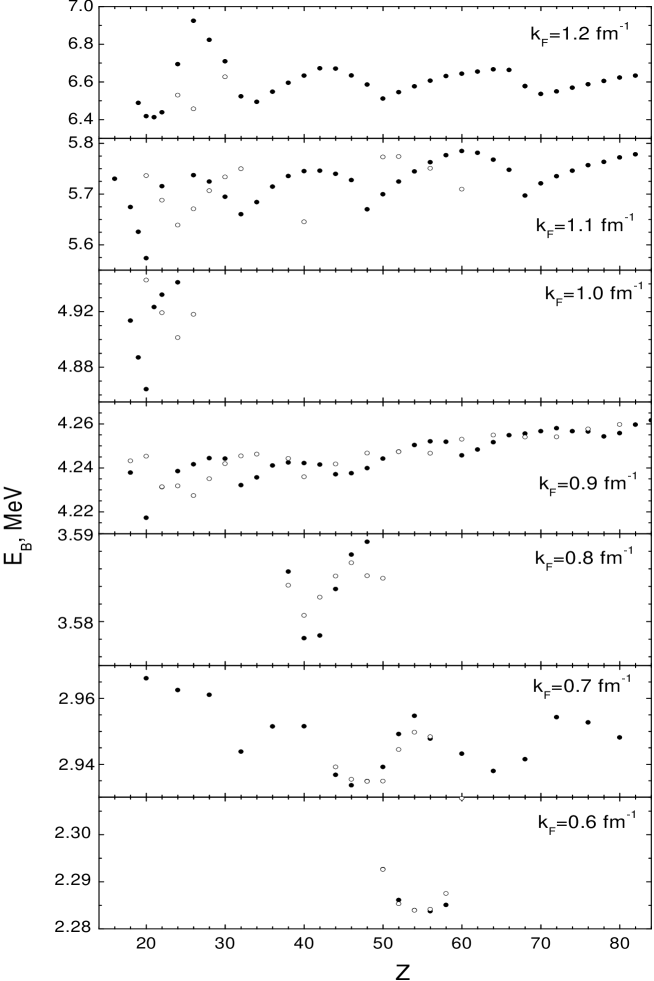
Figure 5: Binding energy per a nucleon for various $k_{\mbox{\scriptsize F}}$ within the P2 model in the case of the BC1 (solid circles) and the BC2 (open circles) kinds of the boundary conditions.

For the case of $k_{\mbox{\scriptsize F}}{=}1.1\;$fm^-1, the $\Delta(r)$ function is displayed in Fig. 6 for the two kinds of boundary conditions. The equilibrium value is $Z{=}20$ in the BC1 case and $Z{=}24$ in the BC2 one. As one can see, the difference between predictions of the two kinds of boundary conditions is drastic. The most strong variation of the gap occurs in the case of $Z{=}20$. To understand the reason of this effect, it is instructive to examine the neutron single particle spectrum $\varepsilon_{\lambda}$. It is displayed in Fig. 7 for the BC1 version and the BC2 one. The positions of the chemical potential $\mu_{n}$ are shown with dots. The two spectra are essentially different. The reason is the shift $\delta\varepsilon_{\lambda}$ of each $\lambda$-level going from BC1 to BC2 version. The value of the shift is approximately equal to one half of the distance between two neighboring levels with the same ($l,j$), the sign of the shift being opposite for even and odd $l$. The absolute value of the shift is proportional to $1/R_{c}^{2}$ and grows at increasing values of $k_{\mbox{\scriptsize F}}$. These shifts are shown for two states, 2$j_{13/2}$ and 1$n_{23/2}$, which are the neighbors of $\mu_{n}$ in the BC1 case. One can see that in both cases there is a shell type structure with rather wide intervals between some neighboring levels. In the BC1 case, we deal with a big inter-level space just at Fermi surface, $\mu_{n}$ being inside. The width of this interval exceeds the value of $2\Delta_{\rm inf}\simeq 2.5\;$MeV which is characteristic for the gap equation. That is why the gap equation in the BC1 case has practically zero solution ($\Delta_{\rm F}<<\Delta_{\rm inf}$). In the BC2 case, big intervals are situated far from the Fermi surface and do not influence significantly the gap equation. Therefore we have a normal situation in this case with $\Delta_{\rm F}\simeq\Delta_{\rm inf}$. For $Z{=}24$ which is the equilibrium value for the BC2 case, the difference between predictions of the BC1 and BC2 versions is not so dramatic but also exists.

Let us return to the P1 model (Table 2). One can see that in the case of $k_{\mbox{\scriptsize F}}{=}1.1\;$fm^-1 and $Z{=}20$ the Fermi average gap value $\Delta_{\rm F}$ is suppressed in comparison with the normal one, but is not zero. For the solution of the gap equation one can use the same spectrum $\varepsilon_{\lambda}$ displayed in Fig. 7. Indeed, the only difference between P1 and P2 models at a fixed value of $Z$ is the value of the gap in neutron matter, $\Delta^{0}_{\rm inf}$, which is a parameter of the model. In the P1 model it is about two times larger than that in the P2 model. However, the direct influence of the gap on the mean field potential and the single-particle spectrum is negligible. But now the value $2\Delta_{\rm inf}\simeq 5\;$MeV is of the order of the energy interval under discussion. Therefore the suppression effect in the gap equation is less than the one in the P2 model.

The “Shell effect” in the neutron single-particle spectrum was discussed in detail in [12]. It was interpreted there as an artifact of the WS approach which does not take into account the periodicity of the crystal. It should disappear in a more consistent approach to the neutron star inner crust structure with periodical boundary conditions. A recipe was suggested in [12] for improving this drawback and finding the gap $\Delta(r)$ in such anomalous cases with big difference of the gap values in the BC1 and BC2 versions, one of them being strongly suppressed. It is based on the smooth dependence of $\Delta(r)$ on $Z$ in a regular situation and consists in the use of $\Delta(r)$ for a neighboring $Z$ with a regular single-particle spectrum at the Fermi surface. In the case under consideration, Fig. 6, the solid line (BC1) for $Z{=}24$ or the dashed one (BC2) for $Z{=}20$ correspond to the “normal” situation. The difference between these two curves is not greater than 10%, and, within such accuracy, any of them could be used as the prediction for $\Delta(r)$ in the case of $k_{\mbox{\scriptsize F}}{=}1.1\;$fm^-1 within the P2 model. As it was discussed in [12], such a recipe is not self-consistent within the WS method but it seems to be reasonable from the physical point of view. The arguments were given in this article in favor of the conclusion that the solution of the gap equation in a more consistent approach should be close to the one in the WS approximation in the case of the regular situation for the neutron spectrum.

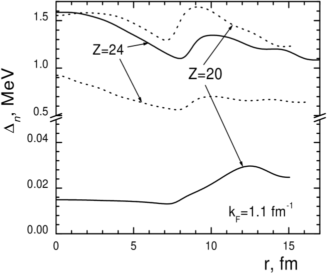
Figure 6: The neutron gap function $\Delta_{n}(r)$ for $k_{\mbox{\scriptsize F}}{=}1.1\;$fm^-1, $Z{=}20$ and $Z{=}24$, in the BC1 case (solid lines) and in the BC2 one (dots), within the P2 model.

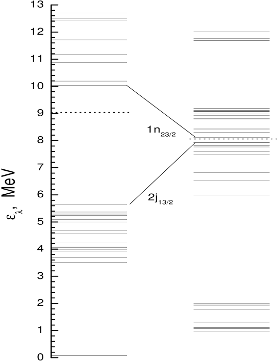
Figure 7: The neutron single-particle spectrum $\varepsilon_{\lambda}$ for $k_{\mbox{\scriptsize F}}{=}1.1\;$fm^-1, $Z{=}20$, in the BC1 case (left) and the BC2 one (right), for the P2 model.

As it is seen in Table 4, at intermediate densities, $k_{\mbox{\scriptsize F}}{=}0.6\div 0.8\;$fm^-1, the regular situation takes place with the approximate equality $\Delta_{\rm F}\simeq\Delta_{\rm inf}$ for both kinds of boundary conditions and $\Delta_{\rm F}^{\rm BC1}\simeq\Delta_{\rm F}^{\rm BC2}$. Therefore one can expect that the gap function $\Delta_{n}(r)$ will be approximately the same in the BC1 and BC2 cases. At $k_{\mbox{\scriptsize F}}{=}0.8\;$fm^-1, where the equilibrium $Z$ value is the same in both versions, these functions are displayed in Fig. 8. In this case the difference between $\Delta_{\rm F}^{\rm BC1}$ and $\Delta_{\rm F}^{\rm BC2}$ is about 10%. As it can be seen in Fig. 8, the difference $\Delta_{n}^{\rm BC1}(r)-\Delta_{n}^{\rm BC2}(r)$ is also about 10% with the exception of small $r<3\;$fm which doesn’t contribute appreciably to the matrix elements of $\Delta_{n}$. Thus, the accuracy of predictions for the gap function within the WS approach in the P2 model for the density interval under consideration is about 10%. Fig. 9 collects the predictions for the gap functions for these values of $k_{\mbox{\scriptsize F}}$ which are taken in accordance with the prescription of Section 3, i.e. those for the BC1 kind of boundary conditions.

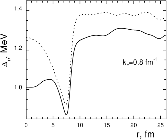
Figure 8: The neutron gap function $\Delta_{n}(r)$ for $k_{\mbox{\scriptsize F}}{=}0.8\;$fm^-1, $Z{=}40$, for the P2 model in the BC1 case (solid line) and in the BC2 one (dashed line).

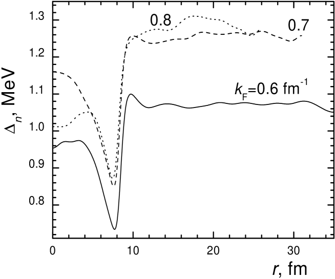
Figure 9: The neutron gap $\Delta_{n}(r)$ for $k_{\mbox{\scriptsize F}}{=}0.6\div 0.8\;$fm^-1 in the case of the P2 model.

Let us go to higher density values, $k_{\mbox{\scriptsize F}}\geq 0.9\;$fm^-1, where the difference between the self-consistent values of $\Delta_{\rm F}^{\rm BC1}$ and $\Delta_{\rm F}^{\rm BC2}$ is significant. As the above discussion for $k_{\mbox{\scriptsize F}}{=}1.1\;$fm^-1 showed, there are two possibilities for the choice of $\Delta_{n}(r)$ in this case with close results. To be definite, let us use the BC1 version as the basic one if the relation $\Delta_{\rm F}^{\rm BC1}\simeq\Delta_{\rm inf}$ takes place. In the opposite case, $\Delta_{\rm F}^{\rm BC1}<<\Delta_{\rm inf}$, we use the equilibrium $Z^{\rm BC1}$ value and the gap function $\Delta_{n}^{\rm BC2}(r)$ for this $Z$. Corresponding gap functions are displayed in Fig. 10. The analysis similar to that for $k_{\mbox{\scriptsize F}}{=}1.1\;$fm^-1 shows that the accuracy of the predictions for $\Delta_{n}(r)$ is again about 10% and only for $k_{\mbox{\scriptsize F}}{=}1.2\;$fm^-1 it is a little worse.

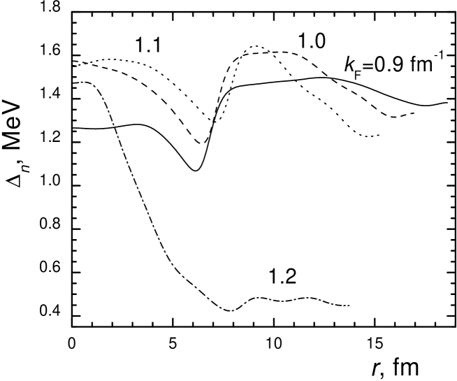
Figure 10: The neutron gap $\Delta_{n}(r)$ for $k_{\mbox{\scriptsize F}}{=}0.9\div 1.2\;$fm^-1 in the case of the P2 model.

5 The P3 model

The P3 model is similar to the P2 one, but now the many-body suppression factor in Eq. (1) is equal to $f_{\rm m-b}{=}1/3$. The calculation scheme and the presentation of results is quite similar to that in the previous section. Values of the binding energy per a nucleon $E_{\rm B}$ in the P3 model are given in Fig. 11 for different densities, $k_{\mbox{\scriptsize F}}{=}0.6\div 1.2\;$fm^-1, similarly to Fig. 5. Again the detailed analysis is made for $k_{\mbox{\scriptsize F}}{=}0.9\;$fm^-1 and partially for $k_{\mbox{\scriptsize F}}{=}0.7\;$fm^-1. Comparison with Fig. 5 shows that positions of the absolute minima of the function $E_{\rm B}(Z)$ are the same as in the P2 model and in the P3 one for both kinds of boundary conditions at all $k_{\mbox{\scriptsize F}}$ values under consideration with only one exception, $k_{\mbox{\scriptsize F}}{=}0.9\;$fm^-1 and the BC2 version. In the latter case the equilibrium $Z$ values differ by 2 units. The main ground state characteristics of the neutron star inner crust within the P3 model are presented in Table 5 which is similar to Table 3 in Section 4 or Table 1 in Section 3. As one can see, the differences between all the values in Table 5 and those in Table 3 are quite small.

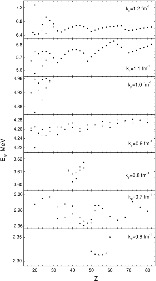
Figure 11: Binding energy per a nucleon for various $k_{\mbox{\scriptsize F}}$ for the P3 model in the case of the BC1 (solid circles) and the BC2 (open circles) kinds of the boundary conditions.

Let us now turn to the analysis of the neutron gap in the P3 model. The corresponding gap characteristics are presented in Table 6 which is similar to Table 4 (the P2 model) or Table 2 (the P1 model). Comparison with Table 4 shows that again the main effect is the general decrease of all the gap characteristics by the factor of 2/3 which corresponds to the values of the many-body suppression factor $f_{\rm m-b}{=}1/3$ in Eq. (1) in the P3 model and $f_{\rm m-b}{=}1/2$ in the P2 model. In two previous sections we discussed a pseudo effect of strong suppression of the neutron gap in some cases with high values of $k_{\mbox{\scriptsize F}}\stackrel{{\scriptstyle\scriptstyle>}}{{\phantom{}{}_{\sim}}}1\;$fm^-1. It originates due to non-regular behavior at big $k_{\mbox{\scriptsize F}}$ of the neutron single particle spectra (the “pseudo Shell effect”) in the WS approach. In the P1 model (Section 3) the first case of a moderate suppression occurs at $k_{\mbox{\scriptsize F}}{=}1.0\;$fm^-1, in the P2 model (Section 4), at $k_{\mbox{\scriptsize F}}{=}0.9\;$fm^-1. In addition, in the P2 model, at $k_{\mbox{\scriptsize F}}\geq 1.0\;$fm^-1, the gap almost vanishes in some cases for the BC1 case or the BC2 one. Table 6 shows that in the P3 model this pseudo effect becomes even stronger, namely, the first case of vanishing occurs at $k_{\mbox{\scriptsize F}}{=}0.9\;$fm^-1. A typical case of such vanishing is shown in Fig. 12. The way to improve this drawback of the WS method and to find the neutron gap function $\Delta_{n}(r)$ in such “bad” cases in the P3 model is the same as above. The predictions for $\Delta_{n}(r)$ within the P3 model are displayed in Fig. 13 for $k_{\mbox{\scriptsize F}}{=}0.6\div 0.8\;$fm^-1 and in Fig. 14 for $k_{\mbox{\scriptsize F}}{=}0.6\div 1.2\;$fm^-1. The method to choose the version (BC1 or BC2) at every value of $k_{\mbox{\scriptsize F}}$ is the same as it was suggested in the previous section for the P2 model.

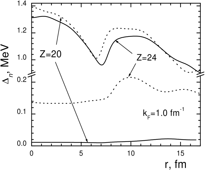
Figure 12: The neutron gap for $k_{\mbox{\scriptsize F}}{=}1.0\;$fm^-1, $Z{=}20$ and $Z{=}24$, in the BC1 case (solid lines) and in the BC2 one (dots), for the P3 model.

Table 5: Comparison of characteristics of equilibrium configurations of the WS cell for two different kinds of the boundary conditions in the case of the P3 model.

$k_{\rm F},$	$\,\,Z\,$	$R_{\rm c},\;$fm		$E_{\rm B},\;$MeV		$\mu_{\rm n},\;$MeV
${\rm fm^{-1}}$		BC1	BC2	BC1	BC2	BC1	BC2
0.6	56	36.92	36.96	2.3132	2.3130	3.5474	3.5634
	54	36.04	36.06	2.3133	2.3121	3.5472	3.5315
0.7	46	30.27	30.27	2.9603	2.9658	4.4009	4.2937
	48	31.09	30.85	2.9630	2.9636	4.3857	4.2913
0.8	40	25.89	26.27	3.6016	3.6079	5.1069	5.1355
0.9	20	18.40	18.62	4.2199	4.2653	6.5184	5.8724
	24	20.11	19.77	4.2592	4.2462	5.9920	5.6863
1.0	20	16.56	16.97	4.8642	4.9581	7.8971	6.8332
	24	18.25	17.85	4.9576	4.9001	7.0551	6.0549
1.1	20	15.05	15.45	5.5735	5.7477	6.2795	7.9492
	24	16.50	16.19	5.7496	5.6340	8.3960	6.7278
1.2	20	15.05	14.23	5.5734	7.2771	6.2792	9.0045
	26	15.30	14.90	6.9276	6.4566	8.9663	8.7410

Table 6: Average gap characteristics in the P3 model

$k_{\rm F},\!\!$	$Z$	$k_{\rm F}^{\rm as},\,{\rm fm^{-1}}$		$\Delta(0),\;$MeV		$\Delta_{\rm as},\;$MeV		$\Delta_{\rm F},\;$MeV		$\Delta_{\rm inf},\;$MeV		$\Delta^{0}_{\rm inf},\!\!$
$\rm fm^{-1}\!\!$		BC1	BC2	BC1	BC2	BC1	BC2	BC1	BC2	BC1	BC2	MeV
0.6	56	0.5817	0.5788	0.721	0.755	0.719	0.713	0.723	0.715	0.778	0.774	0.81
	54	0.5787	0.5792	0.755	0.701	0.732	0.704	0.722	0.713	0.774	0.775
0.7	46	0.6752	0.6782	0.789	0.850	0.832	0.852	0.806	0.865	0.893	0.896	0.92
	48	0.6826	0.6739	0.924	0.765	0.864	0.797	0.864	0.817	0.901	0.891
0.8	40	0.7676	0.7791	0.699	1.019	0.787	0.923	0.799	0.943	0.958	0.964	0.91
0.9	20	0.8489	0.8828	0.080	1.019	0.107	0.887	0.097	0.975	0.974	0.972	0.90
	24	0.8747	0.8450	0.995	0.367	0.817	0.468	0.919	0.479	0.973	0.974
1.0	20	0.9399	0.9690	0.011	1.335	0.019	0.919	0.017	1.100	0.941	0.919	0.89
	24	0.9636	0.9323	1.291	0.134	0.909	0.167	1.068	0.174	0.923	0.947
1.1	20	1.0315	1.060	0.035	1.472	0.028	0.907	0.028	1.154	0.850	0.810	0.75
	24	1.0583	1.0261	1.236	0.618	0.899	0.375	1.10	0.419	0.812	0.858
1.2	20	1.1254	1.1458	1.154	0.010	0.313	0.013	0.418	0.018	0.702	0.661	0.55
	26	1.1308	1.1146	0.157	0.111	0.239	0.021	0.270	0.031	0.691	0.724

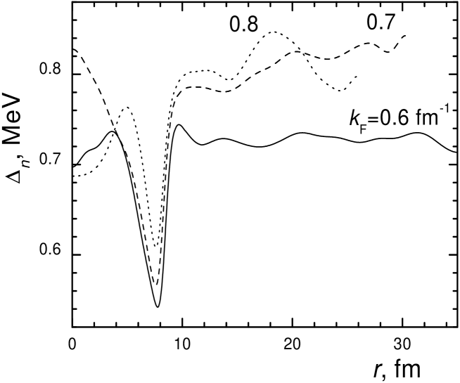
Figure 13: The neutron gap $\Delta_{n}(r)$ for $k_{\mbox{\scriptsize F}}{=}0.6\div 0.8\;$fm^-1 in the case of the P3 model.

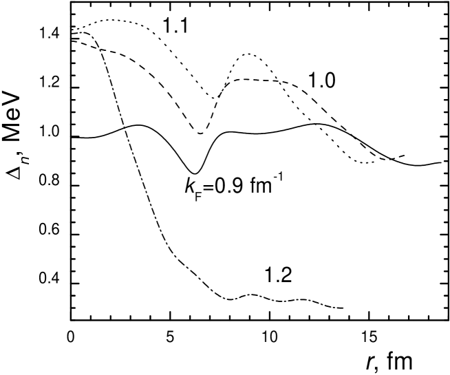
Figure 14: The neutron gap $\Delta_{n}(r)$ for $k_{\mbox{\scriptsize F}}{=}0.9\div 1.2\;$fm^-1 in the case of the P3 model

6 Discussion and Conclusions

Recently a semi-microscopic self-consistent quantum approach was developed [1, 2] for describing the inner crust structure of neutron stars within the WS method with taking into account pairing correlation effects. It is based on the generalized energy functional method [4] which is a modified version of the original Kohn-Sham one [5] for the case of superfluid systems. In this approach, the energy functional is constructed by matching the realistic phenomenological functional by Fayans et al. [4] for describing the nuclear-type cluster in the center of the WS cell to the one calculated microscopically for neutron matter. The anomalous part of the latter was calculated within the BCS approximation. In this paper we take into account, in an approximate way, corrections to the BCS theory which are known from the many-body theory of pairing in neutron matter.

Unfortunately, up to now there is no consistent many-body theory of pairing in neutron matter. However, there exists a conventional point of view [9] that the BCS gap value is suppressed due to various many-body theory corrections significantly, by a factor between 1/2 and 1/3. In the method developed in [1, 2], the set of the neutron matter gap values $\Delta_{n}(k_{\mbox{\scriptsize F}})$ at the Fermi surface for the interval of $0<k_{\mbox{\scriptsize F}}<1.35\;$fm^-1 is the only input to the microscopic part of the superfluid component of the energy functional. In fact, we limit ourselves with the interval of 0.6 fm${}^{-1}<k_{\mbox{\scriptsize F}}<1.2\;$fm^-1 in which the neutron pairing effects are expected to be larger. It is worth to note that the values of $k_{\mbox{\scriptsize F}}\geq 1.1\;$fm^-1 should be considered as optional as far as the WS configuration with spherical symmetry is evidently unstable in this density region [13, 14].

We use a simple model to take into account approximately the many-body corrections to the BCS theory. In this model, the BCS value $\Delta_{n}^{\rm BCS}(k_{\mbox{\scriptsize F}})$ is suppressed by a density independent factor which was taken to be $f_{\rm mb}{=}1/2$ in the first version of the model (named P2) and $f_{\rm mb}{=}1/3$ in the second one, P3. These corrections influence the equilibrium configurations ($Z,R_{c}$) at different $k_{\mbox{\scriptsize F}}$. The maximal variation from the BCS theory (the P1 model) to the P2 version occurs at $k_{\mbox{\scriptsize F}}{=}0.7\;$fm^-1, the equilibrium Z value changing by 6 units. As to the difference of the ($Z,R_{c}$) configurations found within the P2 and P3 models for the same version of the boundary conditions, it is usually negligible. The most important variation for P2 versus P3 occurs in the neutron gap function itself. We think that the realistic situation takes place somewhere between the P2 and P3 models.

7 Acknowlegments

This research was partially supported by the Grant NSh-8756.2006.2 of the Russian Ministry for Science and Education and by the RFBR grant 06-02-17171-a.

References

- [1] M. Baldo, U. Lombardo, E.E. Saperstein, S.V. Tolokonnikov, Nuc. Phys. A 750, 409 (2005).
- [2] M. Baldo, U. Lombardo, E.E. Saperstein, S.V. Tolokonnikov, Phys. At. Nucl. 68, 1812 (2005).
- [3] J. Negele and D. Vautherin, Nucl. Phys. A 207, 298 (1973).
- [4] S.A. Fayans, S.V. Tolokonnikov, E.L. Trykov, and D. Zawischa, Nucl. Phys. A 676, 49 (2000).
- [5] W. Kohn, L.J. Sham, Phys. Rev. A 140, 1133 (1965).
- [6] A. Bulgac and Y. Yu, Int. J. Mod. Phys. E 13, 147 (2004).
- [7] M. Baldo, C. Maieron, P. Schuck and X. Vinas, Nucl. Phys. A 736, 241 (2004).
- [8] R.B. Wiringa, V.G.J. Stoks, R. Schiavilla, Phys. Rev. C 51, 38 (1995).
- [9] M. Baldo, E.E. Saperstein, S.T. Tolokonnikov, Nucl. Phys. A 749, 42 (2005).
- [10] A. Fabrocini, S. Fantoni, A.Y. Illiaronov and K.E. Schmidt, Phys. Rev. Lett. 95, 192501 (2005).
- [11] Y. Yu and A. Bulgac, Phys. Rev. Lett. 90, 161101 (2003).
- [12] M. Baldo, E.E. Saperstein, S.T. Tolokonnikov, Nucl. Phys. A 775, 235 (2006).
- [13] K. Oyamatsu, Nucl. Phys. A 561, 431 (1993).
- [14] P. Magierski, P.-H. Heenen, Phys. Rev. C 65, 045804 (2002).