DEUTERON TENSOR POLARIZATION COMPONENT ${T_{20}(Q^{2})}$ AS A CRUCIAL TEST FOR DEUTERON WAVE FUNCTIONS

Abstract

The deuteron tensor polarization component ${T_{20}(Q^{2})}$ is calculated by relativistic Hamiltonian dynamics approach. It is shown that in the range of momentum transfers available in to-day experiments, relativistic effects, meson exchange currents and the choice of nucleon electromagnetic form factors almost do not influence the value of ${T_{20}(Q^{2})}$. At the same time, this value depends strongly on the actual form of the deuteron wave function, that is on the model of $NN$–interaction in deuteron. So the existing data for ${T_{20}(Q^{2})}$ provide a crucial test for deuteron wave functions.

I Introduction

It is for a long time that in the framework of nonrelativistic approaches deuteron tensor polarization was being considered as an important tool to probe nucleon–nucleon interaction at short distances (see, e.g., Refs. Lev73 ; MoG74 ), giving a possibility to choose between different model deuteron wave functions, that is between different models of $NN$–interaction. During last years great success was achieved in polarization experiments on the elastic electron-deuteron scattering ScB84 ; Dmi85 ; GiH90 ; ThA91 ; FeB96 ; BoA99 ; AbA00 . Now accessible values of $Q^{2}$ are so large that the relativistic theory is needed. Unfortunately, further progress in these measurements is questionable because no reasonable technique exists to extend polarization measurements to higher $Q^{2}$  Gil04 ; GiG02 . So, in the immediate future one does not ezpect any new experimental information on the subject in question.

In the present work we analyze the existing data on polarization $ed$-scattering in connection with different $NN$–interaction models on the base of an essentially relativistic approach. We show that the existing data provide the crucial test of the deuteron wave function even in the relativistic theory. This possibility is based on the following results obtained in the paper.

• The relativistic corrections to $T_{20}(Q^{2})$ are small up to $Q^{2}\simeq 3$(GeV/c)².

• The quantity $T_{20}(Q^{2})$ is almost independent of the actual nucleon electromagnetic form factors (although the deuteron structure functions $A(Q^{2})$ and $B(Q^{2})$ depend strongly).

• The contribution of meson exchange currents (MEC) to $T_{20}(Q^{2})$ are small.

• The quantity $T_{20}(Q^{2})$ depends strongly on the choice of the deuteron wave function, that is on the model of $NN$–interaction.

We consider the most popular model deuteron wave functions to obtain the best description of polarization data.

The analysis is performed in the framework of the variant of the instant form of the relativistic Hamiltonian dynamics (IF RHD) developed by the authors BaK95 ; KrT02 ; KrT03prc ; KrT03 .(RHD is sometimes called Poincaré invariant quantum mechanics (see, e.g., KeP06 .)) The main features of our approach to deuteron are the following. First, the form of the dynamics is close to nonrelativistic case. Second, our method of construction of the matrix element of the electroweak current operator makes it possible to formulate relativistic impulse approximation in such a way that the Lorentz covariance of the current is ensured. In our approach it is possible to use the Siegert theorem Sie37 ; Bai79 to estimate the contribution of meson exchange currents to the deuteron electromagnetic structure. Our estimation of the role of different contributions – nucleon dynamics, relativistic effects, meson exchange currents, nucleon internal structure – demonstrates that one can use the function $T_{20}(Q^{2})$ to discriminate different model deuteron wave functions and to choose the most adequate models of nucleon–nucleon interaction. Our calculation shows that the most popular model wave functions LaL81 ; StK94 ; Mac01 do not give adequate description of $T_{20}(Q^{2})$ and are to be discriminate in favor of those obtained in the dispersion potentialless inverse scattering approach with no adjustable parameters MuT81 ; Tro94 and giving the best description.

The paper is organized as follows. In Section 2 we formulate the problem of obtaining the best deuteron wave function using the data on $T_{20}(Q^{2})$. Section 3 contains a brief review of IF RHD. In Section 4 the electromagnetic deuteron form factors are calculated and the deuteron tensor polarization ${T_{20}(Q^{2})}$ is given in terms of these form factors. The relativistic effects and the effect of MEC are estimated. Section 6 presents the conclusions. In the Appendix A(B) the equations for relativistic (nonrelativistic) free form factors for two nucleons in ${}^{3}S_{1}-^{3}D_{1}$ channel are given. These form factors enter the equations (12) and (13) of the main text.

II Wave functions from deuteron experiments

The problem of obtaining the most adequate wave function from deuteron experimental data, in general, can be correctly formulated only in the conventional nonrelativistic nuclear model. In the framework of this model all existing nucleon–nucleon interaction potentials have the correctly fixed long–distance part defined by the one–pion exchange and the intermediate and the short–distance part of strongly pronounced model character, different in different models. That is why the deuteron wave functions in coordinate representation for different approaches usually coincide at $r\;\geq\;1.5$ fm and differ essentially at $r\;\leq\;0.5$ fm. This quite obvious formulation of the problem in conventional nonrelativistic nuclear model, however, is not valid out of the framework of the approach. This takes place, for example, when relativistic effects are taken into account, or meson exchange currents (interaction currents), or different effects in deuteron electromagnetic structure caused by quark degrees of freedom. These effects are usually strongly model dependent and contain a kind of arbitrariness, so that they “mask” effectively the dependence of observables on the choice of the dynamics of $NN$–interaction. For example, the experimental data on $T_{20}(Q^{2})$ in $ed$-scattering were described well by the relativistic approach of Ref. VaD95 because of functional arbitrariness in the definition of nucleon electromagnetic current. Another example is represented by the calculation of the contribution of meson exchange currents to deuteron electromagnetic from factors where in fact an arbitrariness is contained in the $\rho\pi\gamma$- form factor GaH76 .

Now one understands clearly that it is impossible to neglect relativistic effects in deuteron so that one needs a consistent relativistic formulation of the deuteron problem, particularly at large momentum transfer GiG02 ; ChC88 . As was noted in GiG02 to-day there are two main classes of relativistic schemas of the description of deuteron. The first class is based on field–theoretical concepts ( following the paper GiG02 – propagator dynamics). This class contains the Bethe- Salpeter equation and quasipotential approaches (and the approach  VaD95 , too). The second class – relativistic Hamiltonian dynamics (RHD) – is based on the realization of the Poincaré algebra on the set of dynamical observables of the system with the finite numbers of degrees of freedom. One can find the description of RHD method in the reviews KeP91 (see also Kli98 ) and especially the case of deuteron in the reviews GiG02 ; GaV01 . As is noted in GiG02 , the connection between the propagator dynamics and RHD is ambiguous. Each of the approaches has its own advantages as well as difficulties. One should mention in addition the dispersion methods of describing composite systems, these methods dealing with, in fact, finite numbers of degrees of freedom, as RHD does TrS69 ; KiT75 ; AnK92 ; AnM95 .

In the mentioned relativistic approaches the process of construction of the operator of Lorentz covariant conserved electromagnetic current is connected to the relativistic nucleon-nucleon dynamics used in the approach. That is why the problem of obtaining the information about the dynamics itself from the deuteron data is not, in general, correctly formulated.

Is it possible in principle to formulate correctly the problem of obtaining the most adequate deuteron wave functions from the deuteron experiments? Our opinion is that it is possible if the following requirements are satisfied.

1. It is necessary to find an approach relativistic from the very beginning with the dynamics close to nonrelativistic Schrödinger dynamics, that is with relativistic deuteron wave functions which are close to the nonrelativistic ones.

2. It is necessary to find such a measurable quantity that, in the chosen approach, is almost independent of relativistic corrections, meson exchange currents and the internal structure of nucleons.

In this paper we propose such a relativistic approach – a variant of IF RHD developed by the authors in Refs. BaK95 ; KrT02 ; KrT03prc ; KrT03 . In this approach the adequate observable is the component $T_{20}(Q^{2})$ of the deuteron polarization tensor in elastic electron–deuteron scattering.

Let us review briefly the dynamics in our relativistic approach.

III Dynamics in IF RHD

We use the so called instant form of relativistic Hamiltonian dynamics (IF RHD)  Dir49 . In this form the kinematic subgroup of Poincaré algebra contains the generators of the group of rotations and translations in the three–dimensional Euclidean space (interaction independent generators):

$$\hat{\vec{J}}\>,\quad\hat{\vec{P}}\;.$$ (1)

The remaining generators of the time translation and Lorentz boosts are Hamiltonians (interaction depending):

$$\hat{P}^{0}\>,\quad\hat{\vec{N}}\;.$$ (2)

The additive including of interaction into the mass square operator (Bakamjian–Thomas procedure, see, e.g., KeP91 for details) presents one of the possible technical ways to include interaction in the algebra of the Poincaré group:

$$\hat{M}_{0}^{2}\to\hat{M}_{I}^{2}=\hat{M}_{0}^{2}+\hat{U}\;.$$ (3)

Here $\hat{M}_{0}$ is the operator of invariant mass for the free system and $\hat{M}_{I}$ – for the system with interaction. The interaction operator $\hat{U}$ must satisfy the following commutation relations:

$$\left[\hat{\vec{P}},\,\hat{U}\right]=\left[\hat{\vec{J}},\,\hat{U}\right]=\left[\vec{\bigtriangledown}_{P},\,\hat{U}\right]=0\;.$$ (4)

These constraints (4) ensure that the algebraic relations of Poincaré group are fulfilled for the interacting system. The relations (4) mean that the interaction potential does not depend on the total momentum of the system as well as on the projection of the total angular momentum. The conditions (3) and (4) can be considered only as the model ones. There are other approaches with potential depending on the total momentum but they are out of scope of this paper.

In RHD the wave function of the system of interacting particles is the eigenfunction of a complete set of commuting operators. In IF this set is:

$${\hat{M}}_{I}^{2}\>,\quad{\hat{J}}^{2}\>,\quad\hat{J}_{3}\>,\quad\hat{\vec{P}}\;.$$ (5)

${\hat{J}}^{2}$ is the operator of the square of the total angular momentum. In IF the operators ${\hat{J}}^{2}\;,\;\hat{J}_{3}\;,\;\hat{\vec{P}}$ coincide with those for the free system. So, in Eq.(5) only the operator $\hat{M}_{I}^{2}$ depends on the interaction.

To find the eigenfunctions of the system (5) one has first to construct the adequate basis in the state space of composite system. In the case of two-particle system (for example, two-nucleon system) the Hilbert space in RHD is the direct product of two one-particle Hilbert spaces: ${\cal H}_{NN}\equiv{\cal H}_{N}\otimes{\cal H}_{N}$.

As a basis in ${\cal H}_{NN}$ one can choose the following set of two-particle state vectors where the motion of the two-particle center of mass is separated and where three operators of the set (5) are diagonal:

$$|\,\vec{P},\;\sqrt{s},\;J,\;l,\;S,\;m_{J}\,\rangle\;,$$ (6)

here $P_{\mu}=(p_{1}+p_{2})_{\mu}$, $p_{1}^{2}=p_{2}^{2}=M^{2}$, $M$ is nucleon mass, $P^{2}_{\mu}=s$, $\sqrt{s}$ is the invariant mass of the two-particle system, $l$ – the orbital angular momentum in the center-of-mass frame (C.M.S.), $\vec{S}\,^{2}=(\vec{S}_{1}+\vec{S}_{2})^{2}=S(S+1)\;,\;S$ – the total spin in C.M.S., $J$ – the total angular momentum with the projection $m_{J}$, the parameters $S$ and $l$ play the role of invariant parameters of degeneracy.

As in the basis (6) the operators ${\hat{J}}^{2}\;,\;\hat{J}_{3}\;,\;\hat{\vec{P}}$ in (5) are diagonal, one needs to diagonalize only the operator $\hat{M}_{I}^{2}$ in order to obtain the system wave functions.

The eigenvalue problem for the operator ${\hat{M}}^{2}_{I}$ in the basis (6) coincides with the nonrelativistic Schrödinger equation within following difference between corresponding eigenvalues (see, e.g., ChC88 ; KeP91 ):

$$\left(\frac{M^{2}_{d}}{4\,M}-M\right)-(M_{d}-2M)=\frac{(M_{d}-2M)^{2}}{4\,M}=\epsilon^{2}_{d}/4M\;.$$ (7)

Here $M_{d}$ is the deuteron mass, $\epsilon_{d}$ is the deuteron binding energy.

The difference (7) is negligible for most problems.

The corresponding composite–particle wave function has the form

$$\langle\vec{P}\,^{\prime},\,\sqrt{s^{\prime}},\,J^{\prime},\,l^{\prime},\,S^{\prime},\,m_{J}^{\prime}|\,p_{c}\rangle$$

$$=N_{C}\,\delta(\vec{P}\,^{\prime}-\vec{p}_{c})\delta_{JJ^{\prime}}\delta_{m_{J}m_{J}^{\prime}}\,\varphi^{J^{\prime}}_{l^{\prime}S^{\prime}}(k^{\prime})\;,$$ (8)

$|\,p_{c}\rangle$ is an eigenvector of the set (5); $J(J+1)$ and $m_{J}$ are the eigenvalues of $\hat{J}^{2}\,,\;\hat{J}_{3}\,,$ respectively. $N_{C}$ is the normalization constant.

We use the normalization with the relativistic density of states:

$$k^{2}\,dk\quad\to\quad\frac{k^{2}\,dk}{2\sqrt{(k^{2}+M^{2})}}\;.$$ (9)

This gives the following two–particle wave function of relative motion for equal masses and total angular momentum and total spin fixed:

$$\varphi^{J}_{lS}(k(s))=\sqrt[4]{s}\,u_{l}(k)\,k\;,$$ (10)

with the normalization condition:

$$\sum_{l}\int\,u_{l}^{2}(k)\,k^{2}\,dk=1\;.$$ (11)

Functions $u_{l}(k)\;,\;l=0\;,\;2$ coincide with the model nonrelativistic deuteron wave functions within the difference (7). The wave function (10) coincides with that obtained by “minimal relativization” in FrG89 .

So, in our approach the wave functions in the RHD sense are close to the corresponding nonrelativistic wave functions and the dynamical equation is close to the nonrelativistic Schrödinger equation.

Let us emphasize that our formalism enables one to use any model wave functions obtained as the solution of Schrödinger equation.

In this paper we consider the following models of $NN$–interaction: Paris potential LaL81 , the versions I, II and 93 of the Nijmegen model StK94 , charge–dependent version of Bonn potential Mac01 . The deuteron wave functions for these potentials give the results for deuteron electromagnetic properties that differ essentially from one another. It is a difficult task to give the preference to one of them. Quite different kind of results presents the deuteron wave functions (MT) MuT81 obtained in potentialless approach to the inverse scattering problem (see for the details Tro94 ).

Now let us calculate the deuteron electromagnetic form factors.

IV Deuteron electromagnetic form factors

The main point of our approach is a kind of construction of the matrix element of electroweak current operator. In our method the electroweak current matrix element satisfies the relativistic covariance conditions and in the case of electromagnetic current also the conservation law automatically. The properties of the system as well as the approximations are formulated in terms of form factors. The approach makes it possible to formulate relativistic impulse approximation in such a way that Lorentz covariance of the current is ensured. In the electromagnetic case the current conservation law is also ensured.

Usually it is supposed that it is necessary to take MEC into account in order to provide the gauge invariance and the current conservation KeP91 . However to–day the construction of the relativistic impulse approximation without breaking of the relativistic covariance and current conservation law is a common trend of different approaches GiG02 ; KrT02 ; Kli98 ; LeP00 ; AlK01 . In our approach this is realized by making use of the Wigner–Eckart theorem for the Poincaré group. It enables one (for given current matrix element) to separate the reduced matrix elements (form factors) which are invariant under the Poincaré group action. The matrix element of a given operator is represented as a sum of terms, each one of them being a covariant part multiplied by an invariant part. In such a representation the covariant part describes the transformation properties of the matrix element. The conservation law is satisfied explicitly due to the fact that the vector of the covariant part is orthogonal to the vector $Q_{\mu}$. All the dynamical information on the transition is contained in the invariant part (form factors). In our variant of the impulse approximation (modified impulse approximation) the reduced matrix elements are calculated with no change of covariant part (see KrT02 for the details) although neglecting MEC. The correct transformation properties are thus guaranteed.

Charge, quadrupole and magnetic form factors of deuteron in our approach have the form KrT03prc :

$$G_{C}(Q^{2})=\sum_{l,l^{\prime}}\int\,d\sqrt{s}\,d\sqrt{s^{\prime}}\,\varphi^{l}(s)\,g^{ll^{\prime}}_{0C}(s\,,Q^{2}\,,s^{\prime})\,\varphi^{l^{\prime}}(s^{\prime})\;,$$

$$G_{Q}(Q^{2})\!=\!\frac{2\,M_{d}^{2}}{Q^{2}}\sum_{l,l^{\prime}}\int\!\!d\sqrt{s}\,d\sqrt{s^{\prime}}\,\varphi^{l}\!(s)g^{ll^{\prime}}_{0Q}(s,Q^{2}\!,s^{\prime})\varphi^{l^{\prime}}\!(s^{\prime}),$$ (12)

$$G_{M}(Q^{2})\!=\!-M_{D}\!\sum_{l,l^{\prime}}\int\!\!d\sqrt{s}\,d\sqrt{s^{\prime}}\,\varphi^{l}\!(s)g^{ll^{\prime}}_{0M}(s,Q^{2}\!,s^{\prime})\varphi^{l^{\prime}}\!(s^{\prime}).$$

Here $g^{ll^{\prime}}_{0i}((s\,,Q^{2}\,,s^{\prime})\;,\;i=C,Q,M$ are free charge, quadrupole and magnetic two–particle form factors, that is the form factors describing electromagnetic properties of the system of proton and neutron without interaction, the system having deuteron quantum numbers, $l\;,\;l^{\prime}=$ 0,2, – orbital moments, $\varphi^{l}(s)$ – wave functions in the sense of RHD.

Free two–particle form factors for a system of two fermions with total momentum 1 (without taking into account of $D$-state) were obtained in KrT03prc . Corresponding equations for the neutron–proton system with deuteron quantum numbers are given in Appendix A. Free two–particle charge (only) form factors of proton–neutron system without interaction in deuteron quantum numbers channel are given also in AfA98 .

For the deuteron electromagnetic form factors (12) the correspondence principle is valid. The nonrelativistic limit ($M\;\to\;\infty$) of Eq.(12) gives the standard equations for deuteron form factors in nonrelativistic impulse approximation in terms of wave functions in momentum representation (see, e.g., BrJ76 ; MaZ78 ):

$$G^{N\!R}_{C}(Q^{2})\!=\!\!\sum_{l,l^{\prime}}\!\int\!k^{2}dk\,k^{\prime}\,{}^{2}dk^{\prime}u^{l}(k)\tilde{g}^{ll^{\prime}}_{0C}(k,Q^{2}\!,k^{\prime})u^{l^{\prime}}(k^{\prime}),$$

$$G^{N\!R}_{Q}(Q^{2})\!=\!\frac{2\,M_{D}^{2}}{Q^{2}}\!\sum_{l,l^{\prime}}\!\!\int\!\!k^{2}dk\,k^{\prime 2}dk^{\prime}u^{l}(\!k)\tilde{g}^{ll^{\prime}}_{0Q}\!(k\!,Q^{2}\!\!,k^{\prime})u^{l^{\prime}}\!\!(k^{\prime}),$$ (13)

$$G^{N\!R}_{M}(Q^{2})\!=\!-M_{D}\!\!\sum_{l,l^{\prime}}\!\!\int\!\!k^{2}dk\,k^{\prime}\,{}^{2}dk^{\prime}u^{l}(\!k)\tilde{g}^{ll^{\prime}}_{0M}\!(k\!,Q^{2}\!\!,k^{\prime})u^{l^{\prime}}\!\!(k^{\prime}).$$

Free charge, quadrupole and magnetic two–particle form factors $\tilde{g}^{ll^{\prime}}_{0i}(k\,,Q^{2}\,,k^{\prime})\;,\;i=C,Q,M$ can be calculated as nonrelativistic limits of relativistic two–particle form factors given in Appendix A. The explicit forms of free nonrelativistic two–particle form factors are given in Appendix B.

So, to solve the problem in question we propose the essentially relativistic approach which gives a possibility of calculation of deuteron electromagnetic form factors and takes into account the relativistic covariance and the conservation law for the electromagnetic current. The efficiency of our approach was demonstrated in a number of calculations BaK95 ; KrT02 ; KrT03prc ; KrT03 . In particular, the values of neutron charge form factor extracted from the deuteron charge form factor KrT03 are in good accordance with the values of other authors.

Now let us apply our formalism to polarization $ed$-scattering.

V Polarized $ed$-scattering

The component $T_{20}(Q^{2})$ of the deuteron polarization tensor in elastic $ed$-scattering can be written in terms of deuteron form factors (12) in the following form GiG02 :

$$T_{20}(Q^{2})=-\,\sqrt{2}\frac{Y(Y+2)+X}{1+2Y^{2}+4X}\;,$$ (14)

where

$$Y=\frac{2}{3}\eta\,\frac{G_{Q}(Q^{2})}{G_{C}(Q^{2})}\;,\quad X=\frac{1}{6}\frac{G_{M}^{2}(Q^{2})}{G_{C}^{2}(Q^{2})}\,f(\theta)\;,$$

$$f(\theta_{e})=1+2(1+\eta)\,\tan^{2}\frac{\theta}{2}\;,\quad\eta=\frac{Q^{2}}{4M^{2}_{d}}\;,$$

$\theta$ is the scattering angle in the laboratory frame.

In the range of existing experiments one can neglect $X$ so, that Eq.(14) takes the form:

$$T_{20}(Q^{2})=-\,\sqrt{2}\frac{Y(Y+2)}{1+2Y^{2}}\;.$$ (15)

To elucidate the role of relativistic effects in $T_{20}(Q^{2})$ let us calculate the quantity

$$\Delta(Q^{2})={T^{R}_{20}(Q^{2})}-{T^{NR}_{20}(Q^{2})}\;.$$ (16)

Here $T^{R}_{20}(Q^{2})$ is the relativistic value of $T_{20}(Q^{2})$, calculated according to (14), (12), and $T^{NR}_{20}(Q^{2})$ – is the corresponding nonrelativistic value given by (14), (13).

The dependence of relativistic effects on the choice of the interaction model is shown in Fig. 1.

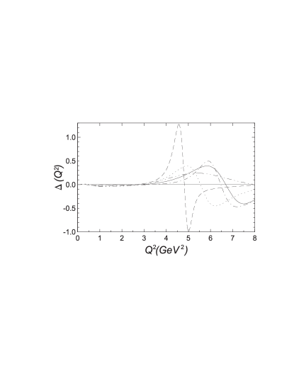
Figure 1: $\Delta(Q^{2})$ calculated following Eq.(1) with nucleon form factors GaK71 and different wave functions. Solid line - N-II StK94 , dashed – MuT81 , dotted – LaL81 , dot-dashed – N-I GiG02 , dashed double–dotted line – Mac01 .

The calculation was made using nucleon form factors GaK71 and different model wave functions. One can see from Fig. 1 that the relativistic effects are small for $Q^{2}\;\simeq$ 3 GeV² for all of wave functions. So, in the region available for the to-day experiment for $T_{20}(Q^{2})$ the relativistic corrections calculated in our approach are small and almost independent of model wave functions. At $Q^{2}\;\geq$ 3.5 GeV² the corrections become larger and depending upon the model.

Let us discuss the role of the nucleon structure. To estimate this role we have calculated $T_{20}(Q^{2})$ for different fits for nucleon form factors. Let us note that one of the fits is that given in GiG02 and taking into account recent data for the ratio of the charge to magnetic form factors for proton $G^{p}_{E}/G^{p}_{M}$, obtained in JLab experiment (see, e.g., Jon00 ).

Relativistic $T_{20}(Q^{2})$ calculated with the use of different nucleon form factors and with MT wave functions obtained through the potentialless approach to inverse scattering problem in MuT81 (see also Tro94 ) is shown in Fig. 2.

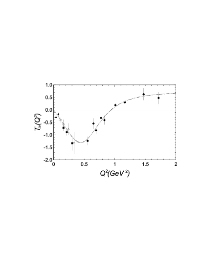
Figure 2: $T_{20}(Q^{2})$ calculated with MT wave functions MuT81 and different nucleon form factors. Solid line - GaK85 , dashed – GaK71 , dotted – MeM96 , dot–dashed – GiG02 , dashed double–dotted – Lom01 . The lines are almost indistinguishible. Experimental data: open circles – ScB84 , open squares – FeB96 , open triangles – GiH90 , filled circles – ThA91 , filled squares – BoA99 , filled diamonds – AbA00 , filled triangles – Dmi85 .

From Fig.2, one can see, as one would expect (see, e.g., the discussion in Ref. GiG02 ), that the dependence on the fit for nucleon form factors is weak. Note, that this result does not depend on the form of wave functions used in the calculation. So, $T_{20}(Q^{2})$ depends weakly on the nucleon structure.

Let us discuss possible contributions to $T_{20}(Q^{2})$ of two–particle MEC.

It is accepted generally that one has to take MEC into account in a way compatible with the basic principles of the chosen approach. So, the value of MEC corrections is different for different approaches. We hope that we can neglect MEC in our approach when the relativistic corrections are small. The base for this is given by the following theorem (Siegert, Sie37 ; see especially the case of deuteron in Bai79 ). If the electromagnetic current satisfies the conservation law in the differential form and if the dynamics of the two–particle system is of nonrelativistic type then the charge density of the exchange current (the null component) is zero independently of the kind of the potential. So, in the range of the energy where the nonrelativistic dynamics is valid (the continuity equation is valid everywhere) the exchange current contributions to the charge and quadrupole form factors are zero. We suppose that when the nonrelativistic dynamics is valid approximately then the MEC contributions to $T_{20}(Q^{2})$ are small.

In the experimental range of $Q^{2}$ the approximate equation (15) is valid for $T_{20}(Q^{2})$, so that this quantity is a function of charge and quadrupole form factors only. This means that MEC contribution to $T_{20}(Q^{2})$ is small.

So, in our approach, the quantity $T_{20}(Q^{2})$ depends weakly on relativistic effects, on meson exchange currents and on nucleon internal structure. This quantity is defined mainly by the choice of the deuteron wave function, so that polarization experiments really could be the test experiments for these wave functions. One can use the experimental data for $T_{20}(Q^{2})$ to choose the most adequate deuteron wave functions. In fact, we have made calculations using different model wave functions to compare the predictions with the experiment. Fig.3 presents the results of our calculation of $T_{20}(Q^{2})$ with the use of the different wave functions LaL81 ; StK94 ; Mac01 ; MuT81 and nucleon form factors from GiG02 as well as the experimental points from the papers ScB84 ; Dmi85 ; GiH90 ; ThA91 ; FeB96 ; BoA99 ; AbA00 .

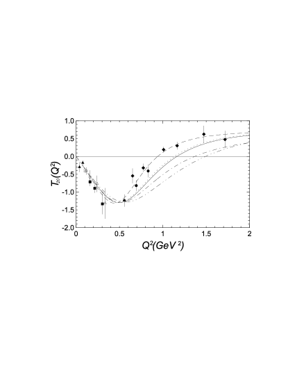
Figure 3: Experimental data (legend as in Fig.1) and $T_{20}(Q^{2})$ calculated with nucleon form factor GaK71 and different wave functions (legend as in Fig. 2).

The calculation was made with the use of nucleon form factors obtained in the paper GaK71 . One can see that the results are strongly model dependent and the best description of experimental data is obtained with the wave functions obtained by the potentialless approach to inverse scattering problem MuT81 . The results for different models coincide only at $Q^{2}\;\leq$ 0.5 GeV². The recent experimental data AbA00 unambiguously choose the MT wave functions MuT81 in comparison with the model wave functions LaL81 ; StK94 ; Mac01 , which are the most largely used now in nuclear calculations.

The important feature of MT-wave functions is the fact that they are “almost model independent”: no form of $NN$–interaction Hamiltonian is used. However, the MT wave functions are given by the dispersion type integral directly in terms of the experimental scattering phases and the mixing parameter for $NN$–scattering in the ${}^{3}S_{1}-^{3}D_{1}$ channel. Regge–analysis of experimental data on $NN$–scattering was used to describe the phase shifts at large energy.

It is worth to notice that the MT wave functions were obtained using quite general assumptions about analytical properties of quantum amplitudes such as the validity of Mandelstam representation for deuteron electrodisintegration amplitude. These wave functions have no fitting parameters and can be altered only with the improvement of the $NN$–scattering phase analysis. The MT wave functions were used in nonrelativistic calculation of deuteron form factors BeM83 and for the relativistic deuteron structure in Arn87 .

Let us notice that the construction of these wave functions is closely related to the equations obtained in the framework of the dispersion approach based on the analytic properties of the scattering amplitudes TrS69 ; KiT75 ; AnK92 ; AnM95 (see also KrT02 and especially the detailed version KrT01h ). In fact, this approach is a kind of dispersion technique using integrals over composite–system masses. Let us note that the MT wave functions have been obtained long in advance for the polarization experiments and contain no parameters to be fitted from deuteron properties.

So, in our approach the problem of determination of the behavior of deuteron wave functions at small distances from polarization experiments is solved. Let us note, that in other approaches with different dynamics the good description of $T_{20}(Q^{2})$ also can be achieved. However, in those approaches it seems to be impossible to separate the contributions to $T_{20}(Q^{2})$ of the dynamics itself, of relativistic effects generated by the current operator construction, and effects of nuclear structure. This concerns, for example, the light–front RHD calculations CaK99 . In the approach  CaK99 quite different dynamics is used which gives 16–component deuteron wave function and good description of $T_{20}(Q^{2})$ is achieved because of relativistic corrections.

VI Conclusion

In this paper the deuteron tensor polarization ${T_{20}(Q^{2})}$ is calculated through relativistic Hamiltonian dynamics approach. It is shown that the experimental data for $T_{20}(Q^{2})$ component of deuteron polarization tensor in elastic electron–deuteron scattering up to $Q^{2}\approx 2(GeV/c)^{2}$ can be described in terms of nonrelativistic theory with no account of relativistic effects and meson exchange currents. These data for $T_{20}(Q^{2})$ could be a touchstone for nonrelativistic deuteron wave functions, the results of calculations depending crucially on the choice of wave functions. It is also shown that the wave functions obtained by the dispersion method of potentialless inverse scattering problem give the best results for $T_{20}(Q^{2})$.

Appendix A Relativistic free two–nucleon form factors in ${}^{3}S_{1}-^{3}D_{1}$ - channel

Relativistic two–particle form factors of free (without interaction) $np$- system in the ${}^{3}S_{1}-^{3}D_{1}$–channel are $2\times 2$ matrices. The elements of three corresponding matrices are given below.

Free two-particle charge form–factor (see below for the notations):

$$g^{ll^{\prime}}_{0C}(s,Q^{2},s^{\prime})=R(s,Q^{2},s^{\prime})\,Q^{2}\left[\,(s+s^{\prime}+Q^{2})\left(G^{p}_{E}(Q^{2})+G^{n}_{E}(Q^{2})\right)g^{ll^{\prime}}_{CE}+\right.$$

$$\left.+\frac{1}{M}\xi(s,Q^{2},s^{\prime})\left(G^{p}_{M}(Q^{2})+G^{n}_{M}(Q^{2})\right)g^{ll^{\prime}}_{CM}\right]\;,$$

$$g^{00}_{CE}=\left(\frac{1}{2}\cos\omega_{1}\cos\omega_{2}+\frac{1}{6}\sin\omega_{1}\sin\omega_{2}\right)\;,\quad g^{00}_{CM}=\left(\frac{1}{2}\cos\omega_{1}\sin\omega_{2}-\frac{1}{6}\sin\omega_{1}\cos\omega_{2}\right)\;,$$

$$g^{02}_{CE}=-\frac{1}{6\sqrt{2}}\,\left(P^{\prime}_{22}+2\,P^{\prime}_{20}\right)\sin\omega_{1}\sin\omega_{2}\;,\quad g^{02}_{CM}=\frac{1}{6\sqrt{2}}\,\left(P^{\prime}_{22}+2\,P^{\prime}_{20}\right)\sin\omega_{1}\cos\omega_{2}\;,$$

$$g^{22}_{CE}=\left[\frac{1}{2}\,L_{1}\,\cos\omega_{1}\cos\omega_{2}+\frac{1}{24}\,L_{2}\,\sin(\omega_{2}-\omega_{1})+\frac{1}{12}\,L_{3}\,\sin\omega_{1}\sin\omega_{2}\right]\;,$$

$$g^{22}_{CM}=-\,\left[-\frac{1}{2}\,L_{1}\,\cos\omega_{1}\sin\omega_{2}+\frac{1}{24}\,L_{2}\,\cos(\omega_{2}-\omega_{1})+\frac{1}{12}\,L_{3}\,\sin\omega_{1}\cos\omega_{2}\right]\;.$$ (17)

Quadrupole two-particle charge form–factor:

$$g^{ll^{\prime}}_{0Q}(s,Q^{2},s^{\prime})=\frac{1}{2}R(s,Q^{2},s^{\prime})\,Q^{2}\left[\,(s+s^{\prime}+Q^{2})\left(G^{p}_{E}(Q^{2})+G^{n}_{E}(Q^{2})\right)g^{ll^{\prime}}_{QE}+\right.$$

$$\left.+\frac{1}{M}\xi(s,Q^{2},s^{\prime})\left(G^{p}_{M}(Q^{2})+G^{n}_{M}(Q^{2})\right)g^{ll^{\prime}}_{QM}\right]\;,$$

$$g^{00}_{QE}=\sin\omega_{1}\sin\omega_{2}\;,\quad g^{00}_{QM}=-\,\sin\omega_{1}\cos\omega_{2}\;,$$

$$g^{02}_{QE}=-\,\frac{3}{2\sqrt{2}}\left\{2\,P^{\prime}_{20}\cos\omega_{1}\cos\omega_{2}-P^{\prime}_{21}\sin(\omega_{1}-\omega_{2})+\frac{1}{3}\left(4\,P^{\prime}_{20}-P^{\prime}_{22}\right)\sin\omega_{1}\sin\omega_{2}\right\}\;,$$

$$g^{02}_{QM}=\frac{3}{2\sqrt{2}}\left\{-\,2\,P^{\prime}_{20}\cos\omega_{1}\sin\omega_{2}+P^{\prime}_{21}\cos(\omega_{1}-\omega_{2})+\frac{1}{3}\left(4\,P^{\prime}_{20}-P^{\prime}_{22}\right)\sin\omega_{1}\cos\omega_{2}\right\}\;,$$

$$g^{22}_{QE}=\frac{3}{2}\left\{\,L_{4}\,\cos\omega_{1}\cos\omega_{2}-\,\frac{1}{12}\,L_{5}\,\sin(\omega_{1}-\omega_{2})+\frac{1}{6}\,L_{6}\,\sin\omega_{1}\sin\omega_{2}\right\}\;,$$

$$g^{22}_{QM}=-\,\frac{3}{2}\,\left\{-\,L_{4}\,\cos\omega_{1}\sin\omega_{2}+\frac{1}{12}\,L_{5}\,\cos(\omega_{1}-\omega_{2})+\frac{1}{6}\,L_{6}\,\sin\omega_{1}\cos\omega_{2}\right\}\;,$$ (18)

Magnetic two-particle charge form–factor:

$$g^{ll^{\prime}}_{0M}(s,Q^{2},s^{\prime})=-\,R(s,Q^{2},s^{\prime})\,\left[\,\xi(s,Q^{2},s^{\prime})\left(G^{p}_{E}(Q^{2})+G^{n}_{E}(Q^{2})\right)g^{ll^{\prime}}_{ME}+\right.$$

$$\left.+\left(G^{p}_{M}(Q^{2})+G^{n}_{M}(Q^{2})\right)g^{ll^{\prime}}_{MM}\right]\;,$$

$$g^{00}_{ME}=\sin(\omega_{1}-\omega_{2})\;,$$

$$g^{00}_{MM}=\frac{1}{2\,M}\left\{\left[\gamma_{1}-\frac{1}{2}\left(\gamma_{3}(s,Q^{2},s^{\prime})+\gamma_{3}(s^{\prime},Q^{2},s)\right)\right]\cos\omega_{1}\cos\omega_{2}+\right.$$

$$\left.+\frac{1}{4}\left(\gamma_{2}(s,Q^{2},s^{\prime})+\gamma_{2}(s^{\prime},Q^{2},s)\right)\cos\omega_{1}\sin\omega_{2}+\frac{1}{2}\gamma_{1}\,\sin\omega_{1}\sin\omega_{2}\right\}\;,$$

$$g^{02}_{ME}=-\,\frac{1}{4\sqrt{2}}\left(P^{\prime}_{22}+2\,P^{\prime}_{20}\right)\sin(\omega_{1}-\omega_{2})\;,$$

$$g^{02}_{MM}=\frac{1}{8\sqrt{2}\,M}\left\{-\,\left[2\,P^{\prime}_{20}\gamma_{1}+P^{\prime}_{21}\gamma_{2}+\left(P^{\prime}_{22}-2\,P^{\prime}_{20}\right)\gamma_{3}\right]\cos\omega_{1}\cos\omega_{2}+\right.$$

$$+\left[P^{\prime}_{21}\gamma_{1}+\frac{1}{2}\left(P^{\prime}_{22}-2\,P^{\prime}_{20}\right)\gamma_{2}-2\,P^{\prime}_{21}\gamma_{3}\right]\cos\omega_{1}\sin\omega_{2}+$$

$$+\left[P^{\prime}_{21}\gamma_{1}-\frac{1}{2}\left(P^{\prime}_{22}+6\,P^{\prime}_{20}\right)\gamma_{2}-2\,P^{\prime}_{21}\gamma_{3}\right]\sin\omega_{1}\cos\omega_{2}+$$

$$\left.+\left[2\,P^{\prime}_{20}\gamma_{1}+P^{\prime}_{21}\gamma_{2}-\left(P^{\prime}_{22}+6\,P^{\prime}_{20}\right)\gamma_{3}\right]\sin\omega_{1}\sin\omega_{2}\right\}\;,$$

$$g^{22}_{ME}=-\,\frac{1}{4}\left\{\frac{1}{2}L_{2}\,\cos(\omega_{1}-\omega_{2})+L_{3}\,\sin(\omega_{1}-\omega_{2})\right\}\;,$$

$$g^{22}_{MM}=\frac{1}{8\,M}\left\{\left[-\,L_{7}\,\gamma_{1}-\frac{1}{8}L_{8}\,\left(\gamma_{2}(s,Q^{2},s^{\prime})-\gamma_{2}(s^{\prime},Q^{2},s)\right)+\right.\right.$$

$$\left.+\frac{1}{2}L_{9}\,\left(\gamma_{3}(s,Q^{2},s)+\gamma_{3}(s^{\prime},Q^{2},s)\right)\right]\cos\omega_{1}\cos\omega_{2}+$$

$$+\frac{1}{4}\left[\left(L_{10}(s,Q^{2},s^{\prime})+L_{10}(s^{\prime},Q^{2},s)\right)\gamma_{1}-\,L_{9}\,\left(\gamma_{2}(s,Q^{2},s^{\prime})+\gamma_{2}(s^{\prime},Q^{2},s)\right)-\right.$$

$$\left.-\,L_{8}\,\left(\gamma_{3}(s,Q^{2},s^{\prime})-\gamma_{3}(s^{\prime},Q^{2},s)\right)\right]\cos\omega_{1}\sin\omega_{2}+$$

$$+\frac{1}{4}\left[8\,L_{11}\,\gamma_{1}+L_{12}\,\left(\gamma_{2}(s,Q^{2},s^{\prime})-\gamma_{2}(s^{\prime},Q^{2},s)\right)+\right.$$

$$\left.+L_{13}\,\left(\gamma_{3}(s,Q^{2},s^{\prime})+\gamma_{3}(s^{\prime},Q^{2},s)\right)\right]\sin\omega_{1}\cos\omega_{2}+$$

$$+\frac{1}{2}\left[\left(L_{14}(s,Q^{2},s^{\prime})+L_{14}(s^{\prime},Q^{2},s)\right)\gamma_{1}-\,\frac{1}{4}L_{13}\,\left(\gamma_{2}(s,Q^{2},s^{\prime})+\gamma_{2}(s^{\prime},Q^{2},s)\right)+\right.$$

$$\left.\left.+L_{12}\,\left(\gamma_{3}(s,Q^{2},s^{\prime})-\gamma_{3}(s^{\prime},Q^{2},s)\right)\right]\sin\omega_{1}\sin\omega_{2}\right\}\;.$$ (19)

The following equation is valid for form factors:

$$g^{ll^{\prime}}_{0i}(s,Q^{2},s^{\prime})=g^{l^{\prime}l}_{0i}(s^{\prime},Q^{2},s)\;,\quad i=C,Q,M\;.$$

Notations:

$$R(s,Q^{2},s^{\prime})=\frac{(s+s^{\prime}+Q^{2})}{\sqrt{(s-4M^{2})(s^{\prime}-4M^{2})}}\,\frac{\vartheta(s,Q^{2},s^{\prime})}{{[\lambda(s,-Q^{2},s^{\prime})]}^{3/2}}\frac{1}{\sqrt{1+Q^{2}/4M^{2}}}\;,$$

$$\xi(s,Q^{2},s^{\prime})=\sqrt{ss^{\prime}Q^{2}-M^{2}\lambda(s,-Q^{2},s^{\prime})}\>,$$

$$L_{1}=L_{1}(s,Q^{2},s^{\prime})=P_{20}\,P^{\prime}_{20}+\frac{1}{3}P_{21}\,P^{\prime}_{21}+\frac{1}{12}P_{22}\,P^{\prime}_{22}\;,$$

$$L_{2}=L_{2}(s,Q^{2},s^{\prime})=P_{21}\left(P^{\prime}_{22}-6\,P^{\prime}_{20}\right)-P^{\prime}_{21}\left(P_{22}-6\,P_{20}\right)\;,$$

$$L_{3}=L_{3}(s,Q^{2},s^{\prime})=2\,P_{21}\,P^{\prime}_{21}+4\,P_{20}\,P^{\prime}_{20}-P_{20}\,P^{\prime}_{22}-P_{22}\,P^{\prime}_{20}\;,$$

$$L_{4}=L_{4}(s,Q^{2},s^{\prime})=P_{20}\,P^{\prime}_{20}+\frac{1}{6}\,P_{21}\,P^{\prime}_{21}-\frac{1}{12}P_{22}\,P^{\prime}_{22}\;,$$

$$L_{5}=L_{5}(s,Q^{2},s^{\prime})=P^{\prime}_{21}\left(P_{22}+6\,P_{20}\right)-P_{21}\left(P^{\prime}_{22}+6\,P^{\prime}_{20}\right)\;,$$

$$L_{6}=L_{6}(s,Q^{2},s^{\prime})=8\,P_{20}\,P^{\prime}_{20}+P_{21}\,P^{\prime}_{21}+P_{20}\,P^{\prime}_{22}+P_{22}\,P^{\prime}_{20}\;,$$

$$L_{7}=L_{7}(s,Q^{2},s^{\prime})=P_{21}\,P^{\prime}_{21}+4\,P_{20}\,P^{\prime}_{20}\;,$$

$$L_{8}=L_{8}(s,Q^{2},s^{\prime})=P_{21}\left(P^{\prime}_{22}+2\,P^{\prime}_{20}\right)+P^{\prime}_{21}\left(P_{22}+2\,P_{20}\right)\;,$$

$$L_{9}=L_{9}(s,Q^{2},s^{\prime})=P_{20}\,P^{\prime}_{22}+P_{22}\,P^{\prime}_{20}+4\,P_{20}\,P^{\prime}_{20}\;,$$

$$L_{10}=L_{10}(s,Q^{2},s^{\prime})=P_{22}\,P^{\prime}_{21}+4\,P_{21}\,P^{\prime}_{20}-2\,P_{20}\,P^{\prime}_{21}\;,$$

$$L_{11}=L_{11}(s,Q^{2},s^{\prime})=P^{\prime}_{21}\,P_{20}-P^{\prime}_{20}\,P_{21}\;,$$

$$L_{12}=L_{12}(s,Q^{2},s^{\prime})=P_{20}\,P^{\prime}_{22}-P_{22}\,P^{\prime}_{20}\;,$$

$$L_{13}=L_{13}(s,Q^{2},s^{\prime})=P_{21}\left(P^{\prime}_{22}+2\,P^{\prime}_{20}\right)-P^{\prime}_{21}\left(P_{22}+2\,P_{20}\right)\;,$$

$$L_{14}=L_{14}(s,Q^{2},s^{\prime})=P_{22}\,P^{\prime}_{20}-P_{21}\,P^{\prime}_{21}-2\,P_{20}\,P^{\prime}_{20}\;,$$

$$\gamma_{1}=\gamma_{1}(s,Q^{2},s^{\prime})=(s+Q^{2}+s^{\prime})\,Q^{2}\;,$$

$$\gamma_{2}=\gamma_{2}(s,Q^{2},s^{\prime})=\xi(s,Q^{2},s^{\prime})\frac{(s-s^{\prime}+Q^{2})(\sqrt{s^{\prime}}+2\,M)+(s^{\prime}-s+Q^{2})\sqrt{s^{\prime}}}{\sqrt{s^{\prime}}(\sqrt{s^{\prime}}+2\,M)}\;,$$

$$\gamma_{3}=\gamma_{3}(s,Q^{2},s^{\prime})=\frac{\xi^{2}(s,Q^{2},s^{\prime})}{\sqrt{s^{\prime}}(\sqrt{s^{\prime}}+2\,M)}\;.$$

$\omega_{1}$ and $\omega_{2}$ – the Wigner rotation parameters,

$$\omega_{1}=\arctan\frac{\xi(s,Q^{2},s^{\prime})}{M\left[(\sqrt{s}+\sqrt{s^{\prime}})^{2}+Q^{2}\right]+\sqrt{ss^{\prime}}(\sqrt{s}+\sqrt{s^{\prime}})}\>,$$

$$\omega_{2}=\arctan\frac{\alpha(s,s^{\prime})\xi(s,Q^{2},s^{\prime})}{M(s+s^{\prime}+Q^{2})\alpha(s,s^{\prime})+\sqrt{ss^{\prime}}(4M^{2}+Q^{2})}\>,$$ (20)

where $\alpha(s,s^{\prime})=2M+\sqrt{s}+\sqrt{s^{\prime}}$. $P_{2i}=P_{2i}(z)\;,\;P^{\prime}_{2i}=P_{2i}(z^{\prime})$ – adjoint Legendre functions:

$$P_{20}(z)=\frac{1}{2}\left(3\,z^{2}-1\right)\;,\quad P_{21}(z)=3\,z\sqrt{1-z^{2}}\;,\quad P_{22}(z)=3\left(1-z^{2}\right)\;.$$ (21)

$z\;,\;z^{\prime}$ – the arguments of Legendre functions:

$$z=z(s,Q^{2},s^{\prime})=\frac{\sqrt{s}(s^{\prime}-s-Q^{2})}{\sqrt{\lambda(s,-Q^{2},s^{\prime})(s-4\,M^{2})}}\;,\quad z^{\prime}=z^{\prime}(s,Q^{2},s^{\prime})=-\,z(s^{\prime},Q^{2},s)\;.$$

$\vartheta(s,Q^{2},s^{\prime})=\theta(s^{\prime}-s_{1})-\theta(s^{\prime}-s_{2})$, $\theta$ - step function.

$$s_{1,2}=2M^{2}+\frac{1}{2M^{2}}(2M^{2}+Q^{2})(s-2M^{2})\mp\frac{1}{2M^{2}}\sqrt{Q^{2}(Q^{2}+4M^{2})s(s-4M^{2})}\;.$$

The functions $s_{1,2}(s,Q^{2})$ give the kinematically available region in the plane $(s,s^{\prime})$. They are obtained in KrT02 . $G^{p,n}_{E,M}(Q^{2})$ are Sachs form factors of proton and neutron.

Appendix B Nonrelativistic free two–nucleon form factors in ${}^{3}S_{1}-^{3}D_{1}$ - channel

Nonrelativistic charge two–particle free form factor:

$$\tilde{g}^{ll^{\prime}}_{0C}(k,Q^{2},k^{\prime})=g(k,Q^{2},k^{\prime})\left(G^{p}_{E}(Q^{2})+G^{n}_{E}(Q^{2})\right)\tilde{g}^{ll^{\prime}}_{CE}\;,$$

$$\tilde{g}^{00}_{CE}=1\;,\quad\tilde{g}^{02}_{CE}=\tilde{g}^{20}_{CE}=0\;,$$

$$\tilde{g}^{22}_{CE}=\tilde{P}_{20}\,\tilde{P}^{\prime}_{20}+\frac{1}{3}\tilde{P}_{21}\,\tilde{P}^{\prime}_{21}+\frac{1}{12}\tilde{P}_{22}\,\tilde{P}^{\prime}_{22}\;,$$ (22)

Nonrelativistic quadrupole two–particle free form factor:

$$\tilde{g}^{ll^{\prime}}_{0Q}(k,Q^{2},k^{\prime})=\frac{3}{2}g(k,Q^{2},k^{\prime})\left(G^{p}_{E}(Q^{2})+G^{n}_{E}(Q^{2})\right)\tilde{g}^{ll^{\prime}}_{QE}\;,$$

$$\tilde{g}^{00}_{QE}=0\;,\quad\tilde{g}^{02}_{QE}=-\,\sqrt{2}\,\tilde{P}^{\prime}_{20}\;,\quad\tilde{g}^{20}_{QE}=-\,\sqrt{2}\,\tilde{P}_{20}\;,$$

$$\tilde{g}^{22}_{QE}=\tilde{P}_{20}\,\tilde{P}^{\prime}_{20}+\frac{1}{6}\tilde{P}_{21}\,\tilde{P}^{\prime}_{21}-\frac{1}{12}\tilde{P}_{22}\,\tilde{P}^{\prime}_{22}\;,$$ (23)

Nonrelativistic magnetic two–particle free form factor:

$$\tilde{g}^{ll^{\prime}}_{0M}(k,Q^{2},k^{\prime})=-\,\frac{1}{4\,\sqrt{2}\,M}g(k,Q^{2},k^{\prime})\left[\left(G^{p}_{E}(Q^{2})+G^{n}_{E}(Q^{2})\right)\tilde{g}^{ll^{\prime}}_{ME}+\right.$$

$$\left.+\left(G^{p}_{M}(Q^{2})+G^{n}_{M}(Q^{2})\right)\tilde{g}^{ll^{\prime}}_{MM}\right].$$

$$\tilde{g}^{00}_{ME}=\tilde{g}^{02}_{ME}=\tilde{g}^{20}_{ME}=0\;,$$

$$\tilde{g}^{00}_{MM}=4\,\sqrt{2}\;,\quad g^{02}_{MM}=-\,{2}\,\tilde{P}^{\prime}_{20}\;,\quad g^{20}_{MM}=-\,{2}\,\tilde{P}_{20}\;,$$

$$\tilde{g}^{22}_{ME}=\gamma\left[\tilde{P}_{21}\,\left(\tilde{P}^{\prime}_{22}-6\,\tilde{P}^{\prime}_{20}\right)-\tilde{P}^{\prime}_{21}\,\left(\tilde{P}_{22}-6\,\tilde{P}_{20}\right)\right]\,$$

$$g^{22}_{MM}=-\,\sqrt{2}\left[\tilde{P}_{21}\,\tilde{P}^{\prime}_{21}+4\,\tilde{P}^{\prime}_{20}\,\tilde{P}_{20}\right]\;.$$ (24)

Here

$$g(k,Q^{2},k^{\prime})=\frac{1}{k\,k^{\prime}\,Q}\left[\theta\left(k^{\prime}-\left|k-\frac{Q}{2}\right|\right)-\theta\left(k^{\prime}-k-\frac{Q}{2}\right)\right]\;.$$

$\tilde{P}_{2i}=P_{2i}(y)\;,\;\tilde{P}^{\prime}_{2i}=P_{2i}(y^{\prime})$ – adjoint Legendre functions (21). $y\;,\;y^{\prime}$ – the arguments of Legendre functions:

$$y=y(k,Q^{2},k^{\prime})=-\,\frac{4(k^{2}-k^{\prime}\,{}^{2})+Q^{2}}{4\,k\,Q}\;,\quad y^{\prime}=y^{\prime}(k,Q^{2},k^{\prime})=-\,y(k^{\prime},Q^{2},k)\;.$$

$$\gamma=-\,\frac{1}{2}\left(\frac{2k^{\prime}\,{}^{2}(1-y^{\prime}\,{}^{2})}{Q^{2}}\right)^{1/2}=-\,\frac{1}{2}\left(\frac{2k^{2}(1-y^{2})}{Q^{2}}\right)^{1/2}\;.$$

References

• (1) J.S.ย Levinger. Acta Phys. 33, 135 (1973); T.J.ย Brady, E.L.ย Tomusiaak, and J.S.ย Levinger, Bull. Amer Phys. Soc. 17, 438 (1972).
• (2) M.J.ย Moravcsik and P.ย Ghosh, Phys. Rev. Lett. 32 321 (1974).
• (3) M.E.ย Schulze, D.ย Beck, M.ย Farkhondeh et al., Phys. Rev. Lett. 52, 597 (1984).
• (4) V.F.ย Dmitriev et al., Phys. Lett. B 157, 143 (1985).
• (5) R.ย Gilman, R.J.ย Holt, E.R.ย Kinney et al., Phys. Rev. Lett. 65, 1733 (1990).
• (6) I.ย The, J.ย Arvieux, D.H.ย Beck et al., Phys. Rev. Lett. 67, 173 (1991).
• (7) M.ย Ferroโ€“Luzzi, M.ย Bouwhuis, E.ย Passchier et al., Phys. Rev. Lett. 77, 2630 (1996).
• (8) M.ย Bouwhuis, R.ย Alarcon, T.ย Botto et al., Phys. Rev. Lett. 82, 3755 (1999).
• (9) D.ย Abbott, A.ย Ahmidouch, H.ย Anklin et al., Phys. Rev. Lett. 84, 5053 (2000).
• (10) R.ย Gilman, Nucl.Phys.A 737, 156 (2004).
• (11) R.ย Gilman and F.ย Gross, J. Phys. G 28, R37 (2002).
• (12) E.V.ย Balandina, A.F.ย Krutov, and V.E.ย Troitsky, J. Phys. G: 22, 1585 (1996); A.F.ย Krutov and V.E.ย Troitsky, J. High Energy Phys. 10, 028 (1999); A.F.ย Krutov, O.I.ย Shro, and V.E.ย Troitsky, Phys. Lett. B 502, 140 (2001), A.F.ย Krutov and V.E.ย Troitsky, Teor. Mat. Fiz. 143, 258 (2005) [Theor. Math. Phys. 143, 704 (2005)].
• (13) A.F.ย Krutov and V.E.ย Troitsky, Phys. Rev. C 65, 045501 (2002).
• (14) A.F.ย Krutov and V.E.ย Troitsky, Phys. Rev. C 68, 018501 (2003).
• (15) A.F.ย Krutov and V.E.ย Troitsky, Eur. Phys. J. A 16, 285 (2003).
• (16) B.D.ย Keister and W.N.ย Polyzou, Phys. Rev. C 73, 014005 (2006).
• (17) A.J.F.ย Siegert, Phys. Rev. 52, 787 (1937).
• (18) H.ย Baier, Fort. Phys. 27, 209 (1979).
• (19) M.ย Lacomb, B.ย Loiseau, R.ย Vinh Mau, J.ย Cotรฉ, P.ย Pirรฉs, and R.ย deย Tourreil, Phys. Lett. B 101, 139 (1981).
• (20) V.G.J.ย Stoks, R.A.M.ย Klomp, C.P.F.ย Terheggen, and J.J.ย deย Swart, Phys. Rev. C 49, 2950 (1994).
• (21) R.ย Machleidt, Phys. Rev. C 63, 024001 (2001).
• (22) V.M.ย Muzafarov and V.E.ย Troitsky, Yad. Fiz. 33, 1461 (1981) [Soviet J. Nucl.Phys. 33, 783 (1981)].
• (23) V.E.ย Troitsky, in Proceedings of Quantum Inversion Theory and Applications, Germany, 1993, edited by H.V. von Geramb, Lecture Notes in Physics 467 (Springer, Berlin, 1994), p. 50.
• (24) J.W.ย Van Orden, N.ย Devine, and F.ย Gross, Phys. Rev. Lett. 75, 4369 (1995).
• (25) M.ย Gari and Hย Hyuga, Nucl. Phys. A 264, 409 (1976).
• (26) P.L.ย Chung, F.ย Coester, B.D.ย Keister, and W.N.ย Polyzou, Phys. Rev. C 37, 2000 (1988).
• (27) B.D.ย Keisterย andย W.ย Polyzou, Adv. Nucl. Phys. 20, 225 (1991).
• (28) W.H.ย Klink, Phys. Rev. C 58, 3587 (1998).
• (29) M.ย Garcon and J.W.ย Van Orden, Adv. Nucl. Phys. 26, 293 (2001).
• (30) V.E.ย Troitsky and Yu.M.ย Shirokov, Theor. Math. Fiz. 1, 213 (1969).
• (31) A.I.ย Kirillov , V.E.ย Troitsky , S.V.ย Trubnikov , and Yu.M.ย Shirokov, Fiz. Elem. Chastits At. Yad. 6, 3 (1975) [Sov. J. Part. Nucl. 6, 3 (1975)].
• (32) V.V.ย Anisovich, M.N.ย Kobrinsky, D.I.ย Melikhov, and A.V.Sarantsev, Nucl. Phys. A 544, 747 (1992).
• (33) V.ย Anisovich, D.ย Melikhov, and V.ย Nikonov, Phys. Rev. D 52, 5295 (1995).
• (34) P.A.M.Dirac, Rev. Mod. Phys. 21, 392 (1949).
• (35) L.L.ย Frankfurt, I.L.ย Grach, L.A.ย Kondratyuk, and M.I.ย Strikman, Phys. Rev. Lett. 62, 387 (1989).
• (36) L.M.ย Lev, E.ย Pace, and G.ย Salmรฉ, Phys. Rev. C. 62, 064004 (2000).
• (37) T.W.ย Allen, W.H.ย Klink, and W.N.ย Polyzou, Phys. Rev. C. 63, 034002 (2001).
• (38) A.V.ย Afanasev, V.D.ย Afanasโ€™ev, and S.V.ย Trubnikov, Preprint TJNAF. JLABโ€“THYโ€“98โ€“01. (Newport News, 1998).
• (39) G.E.ย Brown and A.D.ย Jackson, The Nucleonโ€“Nucleon Interaction (Northโ€“Holland, Amsterdam, 1976).
• (40) L.ย Mathelitsch and H.F.K.ย Zingl, Nuovo Cim. 44, 81 (1978).
• (41) S.ย Galster, H.ย Klein, J.ย Moritz, K.H.ย Schmidt, and D.ย Wegener, Nucl. Phys. B 32, 221 (1971).
• (42) M.ย Jones et al. Phys. Rev. Lett. 84, 1398 (2000).
• (43) M.ย Gari and W.ย Krรผmpelman, Z. Phys. A 322, 689 (1985).
• (44) P.ย Mergell, Ulfโ€“G.ย Meissner, and D.ย Drechsel, Nucl. Phys. A 596, 367 (1996).
• (45) E.L.ย Lomon, Phys. Rev. C 64, 035204 (2001).
• (46) I.I.ย Belyantsev, V.K.ย Mitryushkin, P.K.ย Rashidov, and S.V.ย Trubnikov, J. Phys. G 9, 871 (1983).
• (47) R.G.ย Arnold et al., Phys. Rev. Lett. 58, 1723 (1987).
• (48) A.F.Krutov and V.E.Troitsky, hep-ph/0101327.
• (49) J.Carbonell and V.A.ย Karmanov, Eur. Phys. J. A 6, 9 (1999).