Solving the Nosé-Hoover thermostat for Nuclear Pasta

Abstract

In this work we present a calculation of the hamiltonian variables solving the molecular dynamics equations of motion for a system of nuclear matter kept at fixed temperature by using the Nosé-Hoover Thermostat and interacting via a semiclassical potential depending on both positions and momenta.

1 Introduction

At densities just below nuclear saturation density, there may be spatial structures different from the uniformly distributed matter. In events like a supernova core collapse large quantities of neutrinos are produced. As they stream out of the star, coherent scattering out of spatial density fluctuations of neutron rich matter, known as pasta phases, can happen. These structures arise due to the competition among intermediate-range attractive and long-range repulsive forces [1]. Possible shapes include round nuclei, flat plates, rods, and spherical voids [2].

In this work we are interested in solving the dynamical equations for a nuclear system interacting via a realistic potential model depending not only on positions, as usual, but on both positions and momenta and keeping the temperature fixed using the Nosé-Hoover thermostat[3]. We mimic the Pauli principle in a fermionic nucler system by adding a momentum dependent term to the potential [4]. In this way the characteristic phase space repulsion for fermionic nucleons (protons and neutrons) can be included, restricting some of the available dynamical states for the individual particles. Solving this system allows for realistic configurations of neutron rich plasmas in the NVT ensemble.

2 Model Hamiltonian and Method

We model a charge-neutral system with a fixed number of nucleons, $A$, and electrons. The electrons provide a neutralizing background and are described as an almost degenerate free Fermi gas, see below. The Hamiltonian under the Nosé-Hoover method for the extended system in this case can be written as [3]

$${H}_{\rm NH} = \sum_{i=1}^{A}\frac{{\bf P}_{i}^{2}}{2m_{i}}+{V}({R}_{ij},{P}_{ij})+\frac{s^{2}p_{s}^{2}}{2Q}+g\frac{\ln s}{\beta}\,$$ (1)

where ${V}({R}_{ij},{P}_{ij})$ is the potential which depends on both positions and momenta, described below, $s$ is the extended position variable, $p_{s}$ is the momentum conjugate to $s$, $Q$ is the thermal inertial parameter corresponding to a coupling constant between the system and the thermostat taking a value $Q\sim 10^{6}$-$10^{8}$ MeV $(fm/c)^{2}$, we use $g=3A$ as a condition for generating the canonical ensemble in the classical molecular dynamics simulations, $\xi$ is the thermodynamic friction coefficient and $\beta$ is defined as $\beta=1/k_{\rm B}T$.

The total potential energy of the system, $V$, consists of a sum of two-body interactions

$$V=V_{had}+V_{Coulomb}+V_{Pauli}\$$ (2)

where

$$V_{had}=\sum_{i<j}ae^{-R_{ij}^{2}/\Lambda}+\Big{[}b+c\tau_{i}\tau_{j}\Big{]}e^{-R_{ij}^{2}/2\Lambda}\$$ (3)

$$V_{Coulomb}=\sum_{i<j}\frac{e^{2}}{R_{ij}}e^{-R_{ij}/\lambda}\frac{(1+\tau_{i})}{2}\frac{(1+\tau_{j})}{2}\;,$$ (4)

$$V_{Pauli}=d\left(\frac{\hbar}{q_{0}p_{0}}\right)^{3}\sum_{i,j(\neq i)}\exp{\left[-\frac{({R}_{ij})^{2}}{2q_{0}^{2}}-\frac{({P}_{ij})^{2}}{2p_{0}^{2}}\right]}\ \delta_{\tau_{i}\tau_{j}}\delta_{\sigma_{i}\sigma_{j}}\ ,$$ (5)

Here the distance between the particles in phase space is denoted by $R_{ij}=|{\bf R}_{i}\!-\!{\bf R}_{j}|$, $P_{ij}=|{\bf P}_{i}\!-\!{\bf P}_{j}|$ and $\tau_{i}$ represents the ith-nucleon isospin projection on z-axis ($\tau=\!+\!1$ for protons and $\tau=\!-\!1$ for neutrons). $V_{Coulomb}$ corresponds to the screened Coulomb interaction. The screening length, $\lambda$, that results from the slight polarization of the electron gas is arbitrarily set to $\lambda\!=\!10~{}fm$ as in previous works [5][6] [7]. $V_{Pauli}$ is the Pauli potential that incorporates phase space repulsion for fermions by means of the Kronecker deltas in spin and isospin [8]. This interaction model contains the characteristic intermediate-range attraction and short-range repulsion of the nucleon-nucleon force through $V_{had}$ and allows to include the fermionic nature of nucleons.

The parameter set employed is displayed in table 1, adjusted to reproduce the saturation density and binding energy per nucleon of symmetric nuclear matter and neutron matter, and the binding energy of finite nuclei at $T=1$ MeV.

Table 1: Model parameters.

$a$ (MeV)	$b$ (MeV)	$c$(MeV)	$d$(MeV)	$q_{0}$(fm)	$p_{0}$(MeV/c)	$\Lambda$ (fm2)
133	-47	11	29	3	120	1.5

According to the hamiltonian eq.(1) the equations of motion for each nucleon yield

$$\frac{d{\bf R}_{i}}{dt} = \frac{\partial{H}_{\rm NH}}{\partial{\bf P}_{i}}=\frac{{\bf P}_{i}}{m_{i}}+\frac{\partial{V}}{\partial{\bf P}_{i}}\ ,$$ (6)

$$\frac{d{\bf P}_{i}}{dt} = -\frac{\partial{H}_{\rm NH}}{\partial{\bf R}_{i}}=-\frac{\partial{V}}{\partial{\bf R}_{i}}-\xi{\bf P}_{i}\ ,$$ (7)

$$\frac{1}{s}\frac{ds}{dt} = \frac{1}{s}\frac{\partial{H}_{\rm NH}}{\partial p_{s}}=\frac{1}{Q}\frac{\partial{H}_{\rm NH}}{\partial\xi}=\xi\ ,$$ (8)

$$\frac{d\xi}{dt} = \frac{1}{Q}\left\{\sum_{i=1}^{A}\left(\frac{{\bf P}_{i}^{2}}{m_{i}}+{\bf P}_{i}\cdot\frac{\partial{V}}{\partial{\bf P}_{i}}\right)-\frac{g}{\beta}\right\},$$ (9)

with $\xi\equiv\frac{sp_{s}}{Q}\$

We then study the solution of the equations of motion using different methods, like the exponential fitting [9], exponentially fitted symplectic method [10], but we choose the Numerov type integrator algorithm [11] [12] because it allows the best accuracy, giving order 8 or 12 for this kind of hamiltonians.

The energy of the thermostat system is a conserved quantity

$$E_{NH}=\sum_{i=1}^{A}\frac{P_{i}^{2}}{2m}+V+\frac{1}{2}Q{\xi}^{2}+gkTlns=K+V+E_{\xi}+E_{T}$$ (10)

An effective temperature, that fluctuates around the desired initially set temperature $T$, can be defined as

$$T_{\rm eff}=\frac{2}{3Ak_{\rm B}}\sum_{i=1}^{A}\frac{1}{2}{\bf P}_{i}\cdot\frac{d{\bf R}_{i}}{dt}\$$ (11)

Figure 1: Energy per nucleon versus simulation time at $T=1~{}MeV$, $n_{b}=0.016fm^{-3}$ and $Y_{e}=0.2$. From top to bottom we plot $E_{T},E_{NH},K,E_{\xi},V$ per nucleon.

3 Simulation Results

The simulations presented in this work were carried out with fixed baryonic number density, $n_{b}$, lepton fraction, $Y_{e}=\frac{n_{e}}{n_{b}}$ and a fixed number of nucleons, $A$, initially placed in a cubic box of side $L=(A/n_{b})^{1/3}$ at random. To minimize finite size effects we use periodic boundary conditions. Up to 1,000 particles are taken in this work with typical thermalization times of order $10^{5}fm/c$.

As an example of typical low density conditions we consider $n_{b}=0.016fm^{-3}$, which is about a tenth of normal nuclear density, a temperature $T=1~{}MeV$ and a typical electron fraction for neutron rich matter $Y_{e}=0.2$.

The energy of the system is conserved, according to eq. (10), as can be seen in the plot of energy per particle versus time in Fig. 1. The system exhibits characteristic oscillations in the thermostat variables due to the value of $Q$, that it is associated with the heat capacity of the system.

Figure 2: Effective temperature for a configuration of 200 particles at $T_{eff}=1~{}MeV$, baryon density $n_{b}=0.016fm^{-3}$ and $Y_{e}=0.2$ for $Q=10^{6}~{}MeV(fm/c)^{2}$ and $Q=10^{8}~{}MeV(fm/c)^{2}$. See text for details.

In Fig. 2 we plot the effective temperature for a system of $A=200$ particles at $n_{b}=0.016fm^{-3}$, $Y_{e}=0.2$ and two values of Q. The upper curve (dashed line) corresponds to $Q=10^{6}$ MeV $(fm/c)^{2}$ and the lower curve (solid line) to $Q=10^{8}$ MeV $(fm/c)^{2}$. The temperature is set to T=1 MeV for both curves. The upper curve has been biased by adding an offset of $0.5$ MeV for the sake of clarity. By decreasing Q the temperature control is better but leads to rapid oscillations in the energy, which must be carefully considered when studying the dynamical response in energy modes of the system [13].

In the same way in Fig. 3 we plot the thermostat variable ln s for the same cases as in Fig. 2 and again the dashed line corresponds to $Q=10^{6}$ MeV $(fm/c)^{2}$ and the solid line to $Q=10^{8}$ MeV $(fm/c)^{2}$. This illustrates the slow time variation of $E_{T}$ for systems where Q is set bigger.

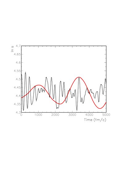
Figure 3: Thermostat variable $lns$ versus simulation time at $T_{eff}=1~{}MeV$, baryon density $n_{b}=0.016fm^{-3}$ and $Y_{e}=0.2$ for $Q=10^{6}~{}MeV(fm/c)^{2}$ and $Q=10^{8}~{}MeV(fm/c)^{2}$. See text for details.

In the numerical simulation the energy of the system may suffer a small drift with time due to the accuracy of the algorithm used. We have checked that the maximum relative extended energy error at time t, defined as

$$\frac{\Delta E}{E}=\left|\frac{E(t)-E(0)}{E(0)}\right|$$ (12)

is $\frac{\Delta E}{E}=10^{-4}$ for time length $\Delta t=5.10^{3}~{}fm/c$ using timesteps $dt=0.025~{}fm/c$ and $Q=10^{6}~{}MeV(fm/c)^{2}$. This error increases somewhat with timestep size. We use timesteps in the range $dt=0.01-0.1~{}fm/c$ for our simulations in this work.

4 Conclusions

In this work we have employed molecular dynamics techniques to solve a hamiltonian model with an interaction potential depending on both positions and momenta. We have simulated neutron rich matter at a given density and kept fixed the temperature by using the Nosé-Hoover thermostat and solved the equations of motion using different integration methods. We find that a Numerov type algorithm allows the best accuracy for this kind of hamiltonians giving order 8 or 12.

We find that at the density of a tenth of nuclear saturation density, $Y_{e}=0.2$ and T=1 MeV a clustered phase is formed. By changing the heat capacity of the system in the range $Q=10^{6}-10^{8}~{}MeV(fm/c)^{2}$ thermalization of the system is achieved in times of order $10^{5}~{}fm/c$. The lower the heat capacity, Q, the better the temperature control is. Induced oscillations in the thermostat variables must be considered with further detail as they could jeopardize low energy excitation modes.

References

- [1] D. G. Ravenhall, C. J. Pethick, and J. R. Wilson, Phys. Rev. Lett. 50, 2066 (1983). M. Hashimoto, H. Seki, and M. Yamada, Prog. Theor. Phys. 71, 320 (1984).
- [2] Gentaro Watanabe, Katsuhiko Sato, Kenji Yasuoka, and Toshikazu Ebisuzaki, Phys. Rev. C 69 055805 (2004)
- [3] S. Bond, B. Leimkulher, B. Laird, Journal of Computational Physics 151 114 (1999) and references therein.
- [4] C. Dorso, S. Duarte, J. Randrup, Phys Lett B 215(1988) 611
- [5] C. J. Horowitz, M. A. Perez-Garcia, and J. Piekarewicz, Phys. Rev. C 69, 045804 (2004).
- [6] C. J. Horowitz, M. A. Perez-Garcia, J. Carriere, D. K. Berry, and J. Piekarewicz, Phys. Rev. C 70 065806 (2004).
- [7] C. J. Horowitz, M. A. Perez-Garcia, D. K. Berry, and J. Piekarewicz, Phys. Rev. C 72 035801 (2005).
- [8] G. Peilert, J. Randrup, H. Stocker, W. Greiner Phys. Let. B 260, 271 (1991).
- [9] J. Vigo-Aguiar, J. Ferrandiz, SIAM J Numer Anal 35 (4), 1684 (1998)
- [10] Simos T.E., J. Vigo-Aguiar, J Phys Rev E 67 (1) 016701 (2003 )
- [11] J. Vigo-Aguiar, H. Ramos, Math. and Computer Modelling, Vol42, 7, 837, (2005)
- [12] J. Vigo-Aguiar, H. Ramos, Journal of Math. Chemistry, 37, 3, 252, (2005)
- [13] C. J. Horowitz, M. A. Perez-Garcia, preprint.