Isoscalar short-range current in the deuteron
induced by an intermediate dibaryon

Abstract

A new model for short-range isoscalar currents in the deuteron and in the $NN$ system is developed; it is based on the generation of an intermediate dibaryon which is the basic ingredient for the medium- and short-range $NN$ interaction which was proposed recently by the present authors. The new current model has only one parameter, which moreover has a clear physical meaning. Our calculations have demonstrated that this new current model can very well describe the experimental data for the three basic deuteron observables of isoscalar magnetic type, viz. the magnetic moment, the circular polarization of the photon in the $\vec{n}p\to d\vec{\gamma}$ process at thermal neutron energies and the structure function $B(Q^{2})$ up to $Q^{2}\simeq$ 60 fm^-2.

I Introduction.

The problem of electromagnetic currents in deuteron, especially of isoscalar nature, still cannot be considered as fully resolved despite of very numerous and longstanding efforts of many groups. As a good example we name here three topics from the field where the present approaches all relying on the conventional nucleon-nucleon ($NN$) force models, failed to explain quantitatively the experimental deuteron data. These are:

• the circular polarization $P_{\gamma}$ of $\gamma$-quanta in radiative capture of spin-polarized neutrons in hydrogen at thermal energies lob ; mul , viz. $\vec{n}+p\to d+\vec{\gamma}$ reaction;

• the deuteron magnetic form factor $B(Q^{2})$ around the diffraction minimum at $Q_{min}\sim$ 50 $fm^{-2}$ sac ; slac ; jlab ; phil ; tjon ;

• the photon-induced polarization of the neutron from the $d(\gamma,\vec{n})p$ reaction at low energysci .

When going to few-nucleon electromagnetic observables the disagreements of modern models for two-body currents with existing experimental data becomes even far more numerous blun . The main part of the above discrepancies is related to the isoscalar magnetic currents which are now still strongly model dependent phil ; tjon ; sci ; blun ; arenh ; carl , and thus cannot be established uniquely. Moreover, the existing theoretical approaches seems to employ all the important types of currents, viz. one-nucleon, two- and three-nucleon ones with many types of meson-exchange currents ($\rho\pi\gamma$, $\omega\pi\gamma$, etc.) to remove the discrepancies. So, the various discrepancies which still remained could imply likely that some important contributions to the electromagnetic currents are still absent. These current components ignored until now are able to remove at least some of the disagreements observed to date in the deuteron- and few-nucleon electromagnetic observables.

In the present paper we propose a model for new currents of isoscalar nature, which still have not been discussed up to date. It is demonstrated below that the new current removes the discrepancies enumerated above in ($i$) - ($ii$) that they make the theoretical framework for electromagnetic properties of the deuteron and the few-nucleon systems more consistent and thus more powerful.

Hence, we shall discuss in Sect. II briefly the status of isoscalar magnetic currents in the deuteron and in the $NN$ system at low energies (see more extended reviews in arenh ; carl ; ris ; marcu ; rho4 ; che ). The dibaryon model for the $NN$ interaction is elaborated in Sect. III where we also include both EFT- and microscopic quark shell-model approaches to substantiate our model. In Sect. IV the properties of deuteron as emerging from the new force model are discussed in detail. We describe the short-range currents induced by the intermediate dibaryon component and the microscopic quark model formalism for the deuteron electromagnetic currents. Sect. V is devoted to a general consideration of the isoscalar $M1$- and $E2$-transition amplitudes and we present in detail the formalism for the isoscalar currents. In particular the formalism for the calculation of the $\vec{n}p{\to}d\gamma$ reaction, the form factor $B(Q^{2})$ and the magnetic moment $\mu_{d}$ is discussed. The numerical results and their comparison to the respective experimental data are presented in Sect. VI. The summary of the results obtained is given in Sect. VII. In the Appendices some useful formulas and some details of the derivation have been collected.

II The status of isoscalar currents in the deuteron

A consistent and correct description of isoscalar currents in the deuteron and in the $NN$-system at very low energy seems to open a door toward quantitative studies of the short-range $NN$-force at low energies. Through this also toward to the non-perturbative QCD at low energies where there are no extra difficulties encountered compared to investigations at high energies, such as a necessity for relativistic treatment, incorporation of many inelastic processes etc. The problem has been first posed by Breit and Rustgi breit many years ago. Main part of the modern efforts to understand the problem quantitatively comes from effective field theory (EFT) treatment in high-orders (N³LO, N⁴LO etc.) and also from the model treatment of short-range $NN$-interaction within phenomenological $NN$-potentials. The point is that the main contribution to the amplitude of processes like $n\!+\!p\to d\!+\!\gamma$ comes from the isovector M1 current. This two-body current is dominated by a long-range $\pi$-meson exchange. This phenomenon has been named in literature as a chiral filter hypothesis rho1 . So, the isovector M1-transitions are “protected by the chiral filter” and does not manifest any sensitivity to short-range interactions.

In the sharp contrast to this, two-body isoscalar current is not protected by the chiral filter and thus depends sensitively on the short-range interactions and short-range current contributions. This renders such currents to be highly model dependent. As a result, within the framework of EFT-approach the treatment of isoscalar currents requires some high orders of ChPT-expansion (N³LO and N⁴LO), which, in turn, introduces some extra parameters rho4 ; che ; rho2 ; rho3 . On the other hand, in a more conventional MEC-treatment (see e.g. blun ; carl ; ris ) the quantitative description of isoscalar currents includes, in addition to the usual $\rho\pi\gamma$-contribution, also the relativistic corrections dependent on the $NN$ interaction model. All these contributions depend crucially upon the meson-nucleon form factor cutoffs $\Lambda_{\pi NN}$, $\Lambda_{\pi N\Delta}$, $\Lambda_{\rho NN}$, $\Lambda_{\omega NN}$ etc. and also upon the electromagnetic form factors of the intermediate mesonsarenh . It is important to emphasize that the above cutoff values chosen for the two-body current models are generally not the same as in the input of $NN$ and 3$N$ potential models sasa and rather often are simply fitted to the electromagnetic observables measured in experiments. The clear evidence to the strongly enhanced values for the cutoffs $\Lambda_{\pi NN}$, $\Lambda_{\pi N\Delta}$, $\Lambda_{\omega NN}$ etc. chosen in traditional $NN$-models like the Bonn potential model can be seen in the results of relativistic calculations for the deuteron structure functions $A(q^{2})$ and $B(q^{2})$, and the deuteron magnetic moment arenh . It is very likely that a serious overestimation of the relativistic contributions found in Ref. arenh indicates to the too high momentum cutoffs in the meson-nucleon vertices.

Thus, one can summarize that the quantitative treatment of isoscalar currents in all existing approaches is related to the rather strong model dependence, in contrast to the isovector M1 current. For example, the experimental value for the circular polarization $P_{\gamma}$ of $\gamma$-quanta emitted in the $np\to d\gamma$ process measured some times ago lob is $P_{\gamma}^{\,exp}\simeq(-1.5\pm 0.3)\times 10^{-3}$ and is underestimated by all existing $NN$- and two-body current models khrip . However, despite of some inner inconsistencies in the two-body current models mentioned above it occurred to be feasible to describe many deuteron electromagnetic observables like static characteristics, charge and quadrupole form factors, the $np\to d\gamma$ cross sections at low energies etc., rather accurately. But the description of other electromagnetic observables, in particularly those given above in the items ($i$) - ($iii$), meets quite serious difficulties.

In particular, there is a long standing puzzle tightly interrelated to the deuteron isoscalar current is a behavior of the deuteron magnetic form factor $B(Q^{2})$ in the area around the diffraction minimum, $Q^{2}\sim$ 45 - 55 $fm^{-2}$. There is a huge literature devoted to calculations of the deuteron form factors. However, the most recent fully relativistic treatment of the $B(Q^{2})$-behavior phil has clearly demonstrated that the existing two-body current models have missed some important contributions. Missing the same contributions very likely is the reason for the visible disagreement of vector and tensor analyzing powers in $p$-$d$ and $n$-$d$ radiative capture at very low energies. Thus, it is evident, there is a number of mutually interconnected effects in the deuteron and the few-nucleon systems where one needs a new isoscalar current. However, the conventional two-body current models still have no appropriate candidates for this.

In this paper we propose an alternative mechanism for isoscalar current generation in the two-nucleon system based on the dibaryon model for $NN$ interactions at intermediate and short ranges developed recently by our group kuk1 ; kuk2 ; kuk6 ; kuk7 . Generally speaking, employment of the dibaryon degree of freedom to describe quantitatively the electromagnetic deuteron properties at low energies is not new. As an example, we shall refer to numerous studies having appeared in 80-ies where authors tried to incorporate various types of six-quark bags to the deuteron wave function to explain some puzzles observed in electromagnetic observables (see, e.g. Refs. yama ; oka ; kissl ; buch ; kobu ). These early attempts have revealed the important role which the quark degrees of freedom plays in the short-range $NN$ interaction and in the electromagnetic structure of deuteron (see, e.g., kobu and references therein). The very important role played by a “hidden color” and the quark pair currents in the deuteron electromagnetic form factors has been established in these works, in particular. However, these early attempts have resulted neither in a deeper understanding of the deuteron electromagnetic observables nor in significant improvement of the description of experimental data.

Very recently, however, in tight interrelation to a renaissance of the dibaryon physics (which is related partially to a recent boom in pentaquark physics), many new studies, both theoretical wang ; pang ; goldm ; pang1 ; ardo ; beane ; flem and experimental khry ; khry1 ; zoln , have appeared in literature. An EFT-approach which included intermediate dibaryons ardo ; beane ; flem focused just on description of electromagnetic properties of the deuteron at low energies and momentum transfer. However, the dibaryons in that approach have been introduced more on formal basis than as a real physical degree of freedom (or an intermediate broad resonance), to improve the convergence of chiral perturbation series and to simplify the EFT scheme in that case. In our dibaryon approach, in contrast to the formal scheme wang ; pang ; goldm ; pang1 , the dibaryons are considered as an important new degree of freedom in the description of $NN$- and 3$N$ interactions in nuclei at intermediate and short ranges kuk1 ; kuk2 ; kuk7 .

The dibaryon concept of the nuclear force at intermediate and short ranges turned out very fruitful in a quantitative or qualitative description of numerous phenomena in hadron and nuclear physics. In particular, this model made it possible to explain without any free parameters the Coulomb displacement energy for $A=$ 3 nuclei (${}^{3}H$ and ${}^{3}He$) and all ground-state characteristics of these nuclei kuk5 ; with exception of the ³H and ³He magnetic moments where we included only single-nucleon currents. However, according to general principle of quantum mechanics, any new degree of freedom must lead to new currents of diagonal and transitional type. On the other hand, in our approach the weight of the dibaryon component in deuteron does not exceed 2.5 - 3.5%. Therefore, just the transitional current from the $NN$ to the dibaryon component can be more important than the diagonal dibaryon current. Nevertheless, we have considered in the present study the diagonal dibaryon current as well.

III The dressed bag model for the medium- and short-range $NN$ interaction

A few key points have been taken as the physical justification of this dibaryon model.

• Failure of the $\sigma$-meson exchange to describe the strong intermediate-range attraction in the $NN$ channel kais ; oset ; kasku . Instead of a strong attraction required by the $NN$-phase shifts, the exchange of two correlated pions with the $S$-wave broad $\sigma$-meson resonance in $\pi$-$\pi$ scattering included to the mechanism, when treated consistently and with a rigor, leads to a strong medium-range repulsion and a weak long-range attraction. Thus, the crucial problem arises, how to explain the basic strong attraction between two nucleons at intermediate range.

• The heavy-meson exchange with the mass $m_{\rho,\omega}\sim$ 800 MeV corresponds in general to the inter-nucleon distances $r_{NN}\sim$ 0.3 fm, i.e. it occurs deeply inside the overlap region between two nucleons. And thus, these exchanges should be consistently treated only with invoking a six-quark dynamics. The ignorance of this dynamics in conventional $NN$-potential approaches (of the OBE type) leads to several serious inconsistencies in OBE-description of short-range $NN$ force (see the discussion in Refs. kuk1 ; kuk2 ; krebl ) and is also a reason for some problems with description of the short-range $NN$ correlation in nuclei.

• One more serious difficulty is related to the choice of different cutoff parameter values $\Lambda_{\pi NN}$, $\Lambda_{\pi N\Delta}$ etc., when one set is used to describe the elastic $NN$ scattering, another set to fit the pion production cross section in $NN$ scattering and the meson exchange contribution to the two-body current, and a third set to describe the three-body force carl ; kuk1 ; kuk2 . Using these different values for the identical vertices in the description of tightly interrelated quantities points toward an inadequate framework employed in the underlying model.

The dibaryon model kuk2 ; kuk7 seemingly overcomes the above difficulties with a consistent description of the short-range $NN$ force. Firstly, it employs a rather soft cutoff parameter $\Lambda_{\pi NN}$ (moreover, there is likely no serious sensitivity to these cutoffs in our model). Secondly, the short-range $NN$ interaction is described through a dressed dibaryon dynamics, so that the conventional heavy-meson exchange in $t$-channel plays no serious role in the short-range $NN$-dynamics. And thirdly, the short-range $NN$-correlations in nuclei tested by high-energy probes can consistently be described as an interaction of the probes with the dibaryon as a whole, which may be associated with its inner excitations or de-excitations.

In our approach the virtual dibaryon in the $NN$ system are modeled through generation of a symmetric six-quark configuration $s^{6}[6]_{\scriptscriptstyle X}$ dressed with a strengthened scalar (e.g. $\sigma$-meson) and other (e.g., $\pi$, $\rho$, $\omega$ etc.) fields. It can be schematically illustrated by Fig. 1.

Figure 1: Driving mechanism for the dressed dibaryon generation used as an intermediate state in the short-range $NN$-interaction.

The enhancement of the scalar field in the symmetric six-quark configuration $s^{6}[6]_{\scriptscriptstyle X}$ implies some rearrangement of quark-gluon fields in the region, where two nucleons are totally overlapping. The emergence of a strong scalar-isoscalar field in the six-quark bag induces automatically an isoscalar exchange current in the multi-quark system.

The $\sigma$-meson loops originate mainly from “non-diagonal” transitions from the mixed-symmetry 2$\hbar\omega$-excited configurations $|s^{4}p^{2}[f_{X}][f_{CS}]\rangle$ to the unexcited fully symmetric configuration $|s^{6}[6_{X}]\rangle$ in the six-quark system with emission of a (virtual or real) $\sigma$-meson. In turn, the strongly attractive interaction between the scalar-isoscalar $\sigma$-field and the multi-quark bag results in an enhancement of the attractive very short-range diquark correlations in the multi-quark system. Thus, as a net result of all these highly non-linear effects the mass of the intermediate dibaryon surrounded by the $\sigma$-field gets much lower as compared to the respective bare dibaryon (see the discussion below).

Completely similar to the behavior of nucleonic system in a scalar field, where the scalar exchange may be viewed as a renormalization of the nucleon mass Serot

$$m\to m^{*}=m+v_{s}(0)\rho,$$

where $v_{s}(0)$ is a volume integral of the scalar exchange potential and $\rho$ is the nucleon density, the constituent quark mass in multi-quark system is also reduced due to interaction with the scalar field:

$$v_{s}(0)\sim-g^{2}_{\sigma q}/m_{\sigma}^{2},$$

where $g_{\sigma q}$ is the $\sigma$-quark coupling constant; note $v_{s}(0)<$ 0 . Thus, the dibaryon mass should be renormalized noticeably due to this scalar field mechanism.

The effect of the strong attraction of the $\sigma$-field to the quark core and the resulting mass shift of the multi-quark system is illustrated easily by the anomalously low mass of the Roper resonance $N^{*}$(1440) with positive parity, which lies even lower than the lowest negative parity resonance $N^{*}$(1535). It is widely accepted krebl that the Roper resonance has mainly the structure $|N+\sigma\rangle$. However, in the language of the simple quark shell model, the second positive parity level in the nucleon spectrum corresponds to 2$\hbar\omega$ excited three-quark configurations $|sp^{2}[21]_{X}\rangle$ or $|s^{2}d-(s^{2}2s)[21]_{X}\rangle$. Thus, exactly the same mechanism as in our dibaryon model, i.e. the $\sigma$-meson emission from the 2$\hbar\omega$-excited state of the nucleon $|sp^{2}[21]_{X}\rangle\to|s^{3}[3]_{X}+\sigma\rangle$, leads to a generation of a strong $\sigma$-field and to a significant shift downward of the Roper resonance mass. Without this strong non-linear effect, the mass of the $N^{*}$(1440) would be $\sim$ 500 MeV higher than that found experimentally. This very large shift gives some estimate for the magnitude of the attractive effects which appear in the interaction of the scalar field with fully symmetric multi-quark bag, or in other words, the effect of dressing by the $\sigma$-meson field. At very short $NN$ distances the $qq$ correlations become repulsive due to one-gluon exchange, and jointly with a strongly enhanced quark kinetic energy, this results in effective short-range repulsion in the $NN$-channel. In our approach this repulsive part of non-local $NN$ interaction is modeled by a separable term $\lambda_{0}\varphi_{0S}({\bf r})\varphi_{0S}({\bf r}^{\prime})$ with a large positive coupling constant $\lambda_{0}$ kuk1 ; kuk2 while the form factor $\varphi_{0S}({\bf r})$ is the projection of the six-quark $|s^{6}[6]_{X}\rangle$ state onto the $NN$-channel: $\varphi_{0S}({\bf r})=\langle N\,N|s^{6}[6]_{X}\rangle$.

Such combined mechanism lies fully beyond the perturbative QCD, and we suggest it can be described phenomenologically by dressing the six-quark propagator $G_{6q}(E)$ with $\sigma$-meson loops kuk6 ; kuk7 . The resulting dressed-bag (DB) propagator $G_{DB}(E)$ and the transition vortexes $NN\to DB$ and $DB\to NN$ treated within a microscopic $6q$ model kuk2 lead automatically to a non-local (separable) energy-dependent short-range $NN$ potential $V_{NqN}(r,r^{\prime};E)$

$$V_{NqN} \equiv \langle NN|V_{Nq}|DB(s^{6})\rangle G_{DB}(E)\,\langle DB(s^{6})|V_{qN}|NN\rangle$$ (1)

$$= \varphi(r)\lambda(E)\varphi(r^{\prime}),$$

where the form factors $\varphi(r)$ are deduced from the microscopic $6q$ model while the coupling constant $\lambda(E)$ is determined by a loop integral with the $\sigma$-loop as shown schematically in Fig. 1 kuk2 . This loop integral can be conventionally parametrized in the following Pade form

$$\lambda(E)=\lambda(0)\frac{E_{0}+aE}{E_{0}-E}.$$ (2)

Here the parameters $\lambda(0)$, $E_{0}$ and $a$ can be either calculated from the microscopic $6q$ model or obtained from fits to the phase shifts of $NN$ scattering in the low partial waves. This approach resulted in the Moscow-Tuebingen (MT) potential model of $NN$ interaction kuk1 ; kuk2 .

In a more general treatment recently developed in Refs. kuk6 ; kuk7 the one-pole approximation for $V_{NqN}$ was obtained on the basis of a fully covariant EFT approach. In a more simple version of the model kuk1 ; kuk2 the transition operator $V_{Nq}$ which couples the nucleon-nucleon and dibaryon channels was calculated within a microscopic quark model with employment of the quark-cluster decomposition of the short-range $N$-$N$ wave function. We consider here the $NN\to DB$ transition in terms of this simple model, shown schematically in Fig. 2, where we assume that the coupling between the $NN$ and $DB$ channels is realised on the quark level via a scalar exchange. This scalar interaction can be presented not only through the $\sigma$-meson exchange but also through a quark confinement or another force including even the four-quark instanton-induced interaction of t’Hooft’s type crist .

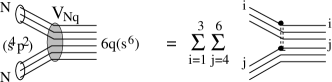
Figure 2: Graphical illustration for $NN\to DB$ transition in terms of quark microscopic model. The double-dashed line denotes some scalar exchange which can induce the $NN\to DB$ transition kuk6 ; kuk7 .

The transition operator $V_{Nq}$ can be written in the form

$$V_{Nq}=\sum_{i\!=\!1}^{3}\sum_{j\!=\!4}^{6}g_{s}^{2}v_{s}(r_{ij}),$$ (3)

where $v_{s}(r_{ij})$ is a scalar $qq$ interaction. This operator should be substituted into the transition matrix element in Eq. (1). The particular form of the scalar operator (3) and its origin are not significant here. The specific mechanism of dressing can also be disregarded at this step since the dressing has already been taken into account in the propagator $G_{DB}$. The most important point is that the S-wave two-cluster state $3q+3q$, which represents the $N$-$N$ system in the overlap region, should be very close in its symmetry to a superposition of the excited six-quark configurations $s^{4}p^{2}$ (see Refs. harv ; obu1 for detail) having non-trivial permutation symmetries with the following Young tableaux in the coordinate- and color-spin spaces $\{f\}\equiv\{[f_{\scriptscriptstyle X}],[f_{\scriptscriptstyle CS}]\}$ ($[f_{\scriptscriptstyle X}]=[6],\,[42],[f_{\scriptscriptstyle CS}]=[42],[321],[2^{3}],[31^{3}],[21^{4}]$). For this reason, we can rewrite the effective $NN$ interaction Eq. (1) generated by the transition operator Eq. (3) in the following constrained form:

$$V_{NqN}(r,r^{\prime};E)\simeq\sum_{ff^{\prime}}\{\langle N(123)|\langle N(456)|\}|s^{4}p^{2}\{f\}\rangle\,\langle s^{4}p^{2}\{f\}|V_{Nq}|s^{6}[6]_{\scriptscriptstyle X}\rangle\\ \times G_{DB}(E)\,\langle s^{6}[6]_{\scriptscriptstyle X}|V_{Nq}|s^{4}p^{2}\{f^{\prime}\}\rangle\,\langle s^{4}p^{2}\{f^{\prime}\}|\,\{|N(123)\rangle|N(456)\rangle\},$$ (4)

where we leave the mixed-symmetry 2$\hbar\omega$-excited six-quark configuration $s^{4}p^{2}$ only (but with all the possible Young tableaux $\{f\}$), instead of the total sum over all the excited six-quark configurations $s^{4}p^{2}$, $s^{2}p^{4}$, …, etc. Then, one can deduce from Eq. (4) that the matrix element of the $NN\to DB$ transition is proportional to the wavefunction of an excited nucleon-nucleon $2S$-state:

$$\{\langle N(123)|\langle N(456)|\}\,|\,s^{4}p^{2}\{f\}\rangle\,=C_{f}\,\varphi_{2S}(r).$$ (5)

Here $C_{f}$’s are purely algebraic coefficients and ${\bf r}=({\bf r}_{1}+{\bf r}_{2}+{\bf r}_{3}-{\bf r}_{4}-{\bf r}_{5}-{\bf r}_{6})/3$ is the relative-motion coordinate of the two $3q$-clusters. For simplicity, we use here the harmonic oscillator (h.o.) $2S$-state function $\varphi_{2S}(r)=2r_{0}^{-3/2}\pi^{-1/4}\sqrt{3/2}\left(2r^{2}/3r_{0}^{2}-1\right)exp(-r^{2}/2r_{0}^{2})$ for the projection of the mixed-symmetry six-quark state onto the $NN$-channel, which is characteristic of the quark shell model. The nucleon wave function N(ijk) in such an approach is described by the pure $s^{3}$ configuration of the CQM

$$|N(123)\rangle\,=|s^{3}[3]_{\scriptscriptstyle X}\{f_{\scriptscriptstyle ST}\}\rangle\\ =\psi_{N}(\rho_{1},\rho_{2})|[2^{3}]_{\scriptscriptstyle C}[3]_{\scriptscriptstyle ST}\rangle,$$ (6)

where $\psi_{N}(\rho_{1},\rho_{2})={\cal N}exp\left[-\frac{1}{2b^{2}}(\rho_{1}^{2}/2+2\rho_{2}^{2}/3)\right]$, the parameter $b$ is the scale parameter of the CQM, with $b\simeq$ 0.5 - 0.6 fm; the relative coordinates are ${\hbox{$\rho$}\hbox to0.0pt{\hss\hbox{$\rho$}\hskip 0.39993pt}\hbox to0.0pt{\hss\lower 0.17218pt\hbox{\hbox{$\rho$}\hbox to0.0pt{\hss\hbox{$\rho$}\hskip 0.39993pt}}}}_{1}={\bf r}_{1}-{\bf r}_{2}$ and ${\hbox{$\rho$}\hbox to0.0pt{\hss\hbox{$\rho$}\hskip 0.39993pt}\hbox to0.0pt{\hss\lower 0.17218pt\hbox{\hbox{$\rho$}\hbox to0.0pt{\hss\hbox{$\rho$}\hskip 0.39993pt}}}}_{2}=({\bf r}_{1}+{\bf r}_{2})/2-{\bf r}_{3}$.

Then, using the 2S function for the transition $NN\to DB$ vertex in Eq. (1), i.e. substituting $\varphi(r)=\varphi_{2S}(r)$, we obtain in our simple ansatz Eq. (3) for the $qq$ pair interaction $v_{s}(r_{ij})$

$$\langle NN(s^{4}p^{2})|V_{Nq}|DB(s^{6})\rangle\,=g_{s}^{2}\,\langle v\rangle\,\varphi_{2S}(r),\\ \mbox{and}\quad\lambda(E)=g_{s}^{4}\,\langle v\rangle^{2}G_{DB}(E),$$ (7)

where $\langle v\rangle$ is a superposition (with the algebraic coefficients $C_{f}$) of the quark shell-model transition matrix elements $\,\langle s^{4}p^{2}|\sum_{i\!=\!1}^{3}\sum_{j\!=\!4}^{6}v_{s}(ij)|s^{6}\!\rangle$.

Note that we did not include the projector $|s^{6}[6]_{\scriptscriptstyle X}\rangle\langle s^{6}[6]_{\scriptscriptstyle X}|$ onto the lowest six-quark configuration $s^{6}[6]_{X}$ in the sum within Eq. (4), because this configuration, according to the most recent $6q$ calculations stan lies well above 2.5 GeV and it is not touched by a strong renormalization, as does the mixed-symmetry state due to strong coupling to the $\sigma$-meson field. Thus, the strong repulsive contribution from the bare intermediate $s^{6}$ bag to the effective short-range $NN$ interaction in the Moscow-Tuebingen (MT) model kuk1 ; kuk2 is modeled by an orthogonality condition to the nodeless 0S state:

$$\int\psi_{NN}(r)\varphi_{0S}(r)d^{3}r=0,$$ (8)

where $\varphi_{0S}$ is a projection of the $6q$-bag state onto the product of nucleon wavefunctions:

$$\varphi_{0S}(r)={\cal N}_{0}^{-1}<\!N(123)|\langle\!N(456)|\}|s^{6}[6]_{\scriptscriptstyle X}\rangle.$$ (9)

Through the orthogonality constraint (8) - (9) the symmetric six-quark bag configuration is excluded from the $NN$ Hilbert space, which prevents a possible double counting of the $s^{6}$ configuration. As a result, the total wavefunction of the two-nucleon system $\Psi_{tot}$ is defined in the direct sum of two Hilbert spaces ${\cal H}_{NN}\oplus{\cal H}_{DB}$. This direct sum can be conventionally represented by the two-line Fock column. For example, the deuteron state in the MT-model reads

$$|d\rangle\,=\left(\begin{array}[]{c}cos\,\theta_{Nq}|d(NN)\rangle\\ \sin\theta_{Nq}|DB\rangle\end{array}\right),$$ (12)

where the mixing angle $\theta_{Nq}$ is calculated on the basis of coupled channel equations with the transition operator $V_{Nq}$ taken as a coupling potential kuk5 . Here the deuteron wavefunction in the $NN$-channel (or the $NN$-component of the deuteron) takes the conventional form

$$|d(NN)\rangle\,=\frac{u(r)}{r}{\cal Y}^{01}_{1M}(\hat{r})+\frac{w(r)}{r}{\cal Y}^{21}_{1M}(\hat{r}),$$ (13)

where the S-wave component $u(r)$ satisfies to the constraint:

$$\int_{0}^{\infty}u(r)\varphi_{0S}(r)dr=0,$$ (14)

The deuteron $NN$-component $|d(NN)\rangle$ and the dibaryon component $|DB\rangle$ are normalized individually to 1. This implies a standard normalization of the total wavefunction

$$\langle d|d\rangle\,=\\ cos^{2}\theta_{Nq}\langle d(NN)|d(NN)\rangle+sin^{2}\theta_{Nq}\langle DB|DB\rangle\ =1$$ (15)

The dressed dibaryon propagator $G_{DB}(E)$ can be represented through the Dyson equation:

$$G_{DB}=G^{(0)}_{DB}+G^{(0)}_{DB}\Sigma\,G_{DB},$$ (16)

where $G^{(0)}_{DB}$ is the bare dibaryon propagator and the $\Sigma$ is an eigenenergy which includes irreducible diagrams, i.e. those which do not include the intermediate free nucleon lines (but still can include $N\Delta$ or $\Delta\Delta$ channels). Our $DB$-model calculations kept only the leading $\sigma$-loop kuk6 ; kuk7 in the series for the $\Sigma$-kernel, because all other graphs (calculated within the six-quark shell model for the quark bag) corresponds to much higher masses (for the details see Refs. kuk6 ; kuk7 ). Moreover, the propagator for the bare six-quark bag $G^{(0)}_{DB}$ corresponds to the pure six-quark bag states with 0$\hbar\omega$ and 2$\hbar\omega$ quanta for even partial waves and 1$\hbar\omega$ for odd partial waves.

When including the $\sigma$-meson loops only into the dressing mechanism, the dressed bag propagator in the one-pole approximation takes the form kuk2 ; kuk5

$$[G_{DB}]^{J}_{LL^{\prime}}=\int d{\bf k}\frac{B_{L}^{J}({\bf k})B_{L^{\prime}}^{J}({\bf k})}{E-E_{\alpha}({\bf k})},$$ (17)

where $B_{L}^{J}({\bf k})$ is the $\sigma DD$ form factor and $E_{\alpha}({\bf k})$ is the total energy of the dressed bag (in the non-relativistic case $E_{\alpha}({\bf k})\simeq m_{\alpha}+\varepsilon_{\sigma}({\bf k})$, with $\varepsilon_{\sigma}({\bf k})=k^{2}/2m_{\alpha}+\omega_{\sigma}({\bf k})\simeq m_{\sigma\alpha}+k^{2}/2m_{\sigma}$, and $m_{\sigma\alpha}=m_{\sigma}m_{\alpha}/(m_{\sigma}+m_{\alpha})$ while $\omega_{\sigma}=\sqrt{m_{\sigma}^{2}+k^{2}}$ is the relativistic energy of $\sigma$-meson). Thus the effective interaction in the $NN$-channel induced by the intermediate dressed dibaryon production takes the form in partial wave representation

$$V_{NqN}=\sum_{JLL^{\prime}}W^{J}_{LL^{\prime}}({\bf r},{\bf r}^{\prime};E)$$ (18)

with

$$W^{J}_{LL^{\prime}}({\bf r},{\bf r}^{\prime};E)=\sum_{M}\varphi^{JM}_{L}({\bf r})\lambda^{J}_{LL^{\prime}}(E)\varphi^{JM}_{L^{\prime}}({\bf r}^{\prime}),\\ \lambda^{J}_{LL^{\prime}}(E)=\gamma^{2}[G_{DB}]^{J}_{LL^{\prime}},$$ (19)

where $\gamma^{2}=g_{s}^{4}\langle v\rangle^{2}$ (see Eqs. (4) - (7) for comparison).

It is easy to show kuk2 ; kuk5 that the weight of the $DB$ in the total $NN$ wavefunction in the $LL^{\prime}SJ$-channel is proportional to the energy derivative

$$\beta^{2}_{LL^{\prime}J}=-\,\frac{\partial\lambda^{J}_{LL^{\prime}}(E)}{\partial E}.$$ (20)

This derivation is in close analogy to a similar procedure for the weight of dressed particle state using the energy derivative of the respective polarization operator $\Pi(P^{2})$ in the field-theory formalism. In particular, recently we developed the fully covariant EFT-derivation kuk6 ; kuk7 for the relativistic $NN$-potential at intermediate and short ranges, similar to Eqs. (17)-(20); we also derived in the simplest one-state approximation a separable form for the relativistic $NN$-interaction in channels ${}^{1}S_{0}$ and ${}^{3}S_{1}$-${}^{3}D_{1}$, which fits almost perfectly the respective $NN$ phase shifts for the large energy interval 0 - 1000 MeV. In contrast to other potentials, e.g. the purely phenomenological Graz separable $NN$ potential which includes a few dozens adjustable parameters for a lesser energy interval this high-quality fit has been performed using only four parameters in the singlet ${}^{1}S_{0}$-channel and a few more for the coupled-channel case ${}^{3}S_{1}-^{3}D_{1}$

Figure 3: Different ways for parameterizing the short-range $NN$ interaction: in low-energy (pionless) EFT through the four-nucleon contact term (left) and in the dibaryon model (right) via $s$-channel intermediate dibaryon.

The separable form of the short-range $NN$ interaction given in Eqs. (18) - (19) can be clearly compared to the contact terms in the effective field theory (EFT) approach (pionless) where all the high-energy physics is parametrized via some contact terms (see Fig. 3, the left graph) which cannot be calculated within that low-energy approach and must be either parametrized somehow phenomenologically or fitted to the data kuk6 ; kuk7 . On the other hand, our short-range mechanism (shown schematically in Fig. 3, right) gives just the energy dependence for such contact terms.

IV Deuteron structure and dibaryon-induced short-range currents

Similar to the general description of the $NN$-system given in Sect. III the total deuteron wavefunction in the DB-model has the form of the Fock column Eq. (12) with at least two components, the $NN$ and the dibaryon dressed with $\sigma$-field — a dressed bag (DB) kuk1 ; kuk2 . The DB-component $|DB>$ in the second line of Eq. (12) can be presented in the graphic form as a superposition of a bare dibaryon (six-quark configuration $s^{6}[6_{X}]$) and an infinite series of $\sigma$-meson loops coupled to the $s^{6}$-quark core propagator. Thus, this component includes both the bare and dressed parts.

Taking further the simple Pade-form (2) of the energy dependent factor $\lambda^{J}_{LL^{\prime}}(E)$ in Eq. (19) and by calculating the energy derivative (20) one gets easily the weight of the dressed dibaryon component in the deuteron, which turns out to be $\beta^{2}\simeq$ 0.025 - 0.035 for different versions of the model. It is very interesting that this weight of the dibaryon component derived from the energy dependence of the $\sigma$-loop diagram is rather close to the weight of non-nucleonic components (e.g. $\Delta\Delta$ etc.) in the deuteron deduced within many phenomenological models. Table 1 gives the summary of the static characteristics of the deuteron found with this dibaryon model kuk2 ; kask .

Table 1: Deuteron properties in different models.

	$E_{d}$	$P_{D}$	$r_{m}$	$Q_{d}$	$\mu_{d}$	$A_{S}$	$D/S$
Model	(MeV)	(%)	(fm)	(fm2)	($\mu_{N}$)	(fm-1/2)
RSC	2.22461	6.47	1.957	0.280	0.8429	0.8776	0.0262
AV18	2.2245	5.76	1.967	0.270	0.8521	0.8850	0.0256
Bonn 2001	2.22458	4.85	1.966	0.270	0.8521	0.8846	0.0256
DB ($NN$ only)	2.22454	5.42	2.004	0.286	0.8489	0.9031	0.0259
DB ($NN$+6q)	2.22454	5.22	1.972	0.275	0.8548	0.8864	0.0264
Experiment	2.22454(9)a		1.971(2)b	0.2859(3)c	0.857406(1)d	0.8846(4)e	0.0264f
	aRef. a ,		bRef. b ,	cRef. c and c1 ,	dRef. d ,	eRef. e ,	fRef. f .

The parameters of the model obtained from fit to the phase shifts of elastic $NN$ scattering in the ${}^{3}S_{1}$ - ${}^{3}D_{1}$ channel have the following values

$$\lambda(0)=-385.89\,\,MeV,\quad E_{0}=855.29\,\,MeV,\\ \quad a=-0.025,\quad r_{0}=0.38113\,\,fm,\quad(b=\sqrt{\frac{3}{2}}r_{0}).$$ (21)

We emphasize here again, that after fitting the phase shifts our approach does not have any free or adjustable parameters left for the description of the deuteron properties. From Table 1 one can see that the predictions for the basic deuteron observables found in the above dibaryon model is generally even in better agreement with respective experimental data than those for the modern $NN$-potentials calculated conventionally.

The modeling of the $NN\to DB$ transition by scalar exchanges between quarks makes it possible to consider the “contact” $\gamma NN\to DB$ vertices (Fig. 4) in terms of CQM with the minimal electromagnetic interaction of the constituent quarks, i.e. with the quark current

$$j^{\mu}_{q}(q) = \sum_{i=1}^{6}\hat{e}_{i}F_{q}(q^{2})\bar{u}(p_{i}^{\prime})\gamma^{\mu}_{i}u(p_{i}),$$ (22)

where $q=p^{\prime}-p$, $\hat{e}_{i}=\frac{1}{6}\!+\!\frac{1}{2}\tau^{(i)}_{z}$ and $F_{q}(q^{2})$ is a form factor of the constituent quark

Figure 4: Schematic representation of the new electromagnetic currents induced by intermediate dibaryon generation.

which can only show itself at intermediate momentum transfer $Q^{2}\gtrsim$ 1 GeV²/c². It implies that the constituent quark is an extended object and has obtained its own electromagnetic form factor, e.g. a monopole one $F_{q}(Q^{2})=1/(1+Q^{2}/\Lambda_{q}^{2})$, where the parameter $\Lambda_{q}$ is expected to be set by the chiral symmetry scale $\Lambda_{\chi}\simeq 4\pi f_{\pi}\simeq$ 1 GeV.

For definiteness, we consider the diagrams (a) and (c) depicted in Fig. 4. In our model with the scalar exchanges and the CQM current (22) these contact terms are equivalent to the sum of Feynman diagrams depicted in Fig. 5. These diagrams describe the two-particle currents in the six-quark system. The diagram ($e$) in Fig. 5 gives rise to an additional (i.e. the $\gamma$-induced) contribution to the transition $s^{4}p^{2}\to s^{6}$ as compared to the mechanism shown in Fig. 2. Here we demonstrate that within the above model for the short-range $NN$ interaction the minimal quark-photon coupling $j^{\mu}_{q}(q)A_{\mu}(q)$ leads to a non-additive two-nucleon current which does not vanish in the low-energy limit $q_{0},|{\bf q}|\to$ 0. In this limit, only the contribution of the diagram Fig. 5(e) vanishes because of orthogonality of the $s^{6}$ configuration to the quark-cluster states in the $N$-$N$ channel (i.e. to the configurations $s^{4}p^{2}$ and the other ones). By contrast, the total contribution of the diagrams ($a$)-($d$) and ($f$) in Fig. 5 does not vanish at $q_{0}\to 0$. In each pair of diagrams, ($a$) and ($b$), depicted in Fig. 6, the singular terms $\sim 1/q_{0}$ are mutually canceled, but the remainder, proportional to the momentum k between the $i$-th and $j$-th quarks and also to the scalar $qq$-interaction potential $v_{s}({\bf k}^{2})$, does not vanish in the limit $q_{0}\to 0$ because of non-vanishing the matrix element $\langle s^{4}p^{2}|v_{s}|s^{6}\rangle$ (see below).

Now we pass to the actual calculations of such diagram contributions. It should be stressed here that the current diagrams in Fig. 5 corresponds just to the ‘non-diagonal’ (transition) electromagnetic current which couples two different channels, i.e. the proper $NN$- and $DB$-channels. These channel wavefunctions enter the transition matrix elements with a proper own normalization because any current associated to the $DB$-state is “normalized” to the weight of the $DB$-component. Among other things this makes it possible to avoid any double counting (symmetry properties of quark configurations are discussed in Appendix A which argue strongly against the repeated contribution in detail). When the spin part of the $i$-th quark current (Eq. 22) is taken into account only and a low energetic $M1$-photon is generated, one can write the following Feynman amplitudes $M^{\lambda}_{ij}$ for the diagrams depicted in Fig. 6($a$) and ($b$)

$$M^{\lambda}_{ij(a)}=\frac{ieg_{s}^{2}v_{s}(k_{j}^{2})}{2m_{q}}\bar{u}(p_{i}^{\prime})\left\{\hat{e}_{i}\sigma_{i}^{\mu\nu}q_{\nu}\varepsilon_{\mu}^{(\lambda)*}\frac{2m_{q}-\!\not k_{i}+\!\not q}{2p_{i}^{\prime}\cdot q}\right.\\ \left.+\frac{2m_{q}+\!\not k_{i}-\!\not q}{-2p_{i}\cdot q}\hat{e}_{i}\sigma_{i}^{\mu\nu}q_{\nu}\varepsilon_{\mu}^{(\lambda)*}\right\}u(p_{i}),\\ M^{\lambda}_{ij(b)}=\frac{ieg_{s}^{2}v_{s}(k_{i}^{2})}{2m_{q}}\bar{u}(p_{j}^{\prime})\left\{\hat{e}_{j}\sigma_{j}^{\mu\nu}q_{\nu}\varepsilon_{\mu}^{(\lambda)*}\frac{2m_{q}-\!\not k_{j}+\!\not q}{2p_{j}^{\prime}\cdot q}\right.\\ \left.+\frac{2m_{q}+\!\not k_{j}-\!\not q}{-2p_{j}\cdot q}\hat{e}_{j}\sigma_{j}^{\mu\nu}q_{\nu}\varepsilon_{\mu}^{(\lambda)*}\right\}u(p_{j}),$$ (23)

where $\varepsilon_{\mu}^{(\lambda)*}$ is a space-like photon polarization vector $\varepsilon^{\mu(\lambda)*}=\{0,{\hbox{$\epsilon$}\hbox to0.0pt{\hss\hbox{$\epsilon$}\hskip 0.39993pt}\hbox to0.0pt{\hss\lower 0.17218pt\hbox{\hbox{$\epsilon$}\hbox to0.0pt{\hss\hbox{$\epsilon$}\hskip 0.39993pt}}}}^{(\lambda)*}\}$ satisfying the transversality condition $\hat{\bf q}\cdot{\hbox{$\epsilon$}\hbox to0.0pt{\hss\hbox{$\epsilon$}\hskip 0.39993pt}\hbox to0.0pt{\hss\lower 0.17218pt\hbox{\hbox{$\epsilon$}\hbox to0.0pt{\hss\hbox{$\epsilon$}\hskip 0.39993pt}}}}^{(\lambda)*}=$ 0 at $\lambda=\pm$ 1.

It is easy to verify that the singular terms $\sigma_{i}^{\mu\nu}q_{\nu}\varepsilon_{\mu}^{(\lambda)*}m_{q}/(p_{i}^{\prime}\cdot q)$ and $\sigma_{i}^{\mu\nu}q_{\nu}\varepsilon_{\mu}^{(\lambda)*}m_{q}/(\!-\!p_{i}\cdot q)$ cancel each other in sum $M^{\lambda}_{ij(a)}+M^{\lambda}_{ij(b)}$ in the limit $q_{0}\to 0$. As a result, we obtain from Eq. (23) in the non-relativistic approximation $q_{0}/m_{q}\ll$ 1 the three-dimensional operator

$$V_{Nq\gamma}=\frac{ieg_{s}^{2}}{2m_{q}}\sum_{i\!=\!1}^{3}\sum_{j\!=\!4}^{6}{\hbox{$\epsilon$}\hbox to0.0pt{\hss\hbox{$\epsilon$}\hskip 0.39993pt}\hbox to0.0pt{\hss\lower 0.17218pt\hbox{\hbox{$\epsilon$}\hbox to0.0pt{\hss\hbox{$\epsilon$}\hskip 0.39993pt}}}}^{(\lambda)*}\cdot\left\{v_{s}({\bf k}^{2}_{j})\left(\frac{\hat{\bf q}\cdot{\bf k}_{i}}{m_{q}}[{\hbox{$\sigma$}\hbox to0.0pt{\hss\hbox{$\sigma$}\hskip 0.39993pt}\hbox to0.0pt{\hss\lower 0.17218pt\hbox{\hbox{$\sigma$}\hbox to0.0pt{\hss\hbox{$\sigma$}\hskip 0.39993pt}}}}_{i}\times\hat{\bf q}]-\frac{[{\hbox{$\sigma$}\hbox to0.0pt{\hss\hbox{$\sigma$}\hskip 0.39993pt}\hbox to0.0pt{\hss\lower 0.17218pt\hbox{\hbox{$\sigma$}\hbox to0.0pt{\hss\hbox{$\sigma$}\hskip 0.39993pt}}}}_{i}\times{\bf k}_{i}]}{m_{q}}\right)+v_{s}({\bf k}^{2}_{i})\left(-\,\frac{\hat{\bf q}\cdot{\bf k}_{j}}{m_{q}}[{\hbox{$\sigma$}\hbox to0.0pt{\hss\hbox{$\sigma$}\hskip 0.39993pt}\hbox to0.0pt{\hss\lower 0.17218pt\hbox{\hbox{$\sigma$}\hbox to0.0pt{\hss\hbox{$\sigma$}\hskip 0.39993pt}}}}_{j}\times\hat{\bf q}]-\frac{[{\hbox{$\sigma$}\hbox to0.0pt{\hss\hbox{$\sigma$}\hskip 0.39993pt}\hbox to0.0pt{\hss\lower 0.17218pt\hbox{\hbox{$\sigma$}\hbox to0.0pt{\hss\hbox{$\sigma$}\hskip 0.39993pt}}}}_{j}\times{\bf k}_{j}]}{m_{q}}\right)\right\}\\ \times(2\pi)^{3}\delta^{3}({\bf p}_{i}+{\bf p}_{j}-{\bf p}^{\prime}_{i}-{\bf p}^{\prime}_{j}-{\bf q})$$ (24)

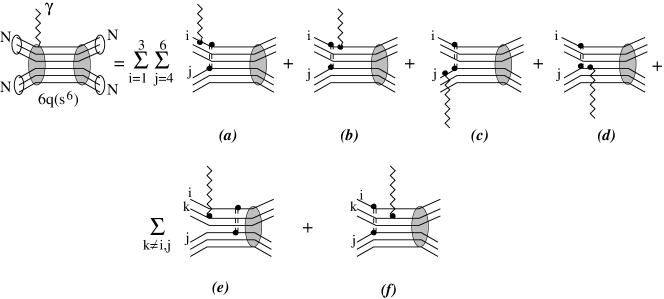
Figure 5: The diagram series illustrating the contact $V_{Nq\gamma}$ terms contributing to the “non-diagonal” current.

defined on non-relativistic quark wavefunctions of the CQM. This operator describes the transition from the $NN$ channel to the $6q$-bag with emission of a $M1$ $\gamma$-quantum, i.e. a “contact” $NN\to DB+\gamma$ interaction, schematically shown in Fig. 4(a).

Now we can calculate the effective contact vertex $NN\Leftrightarrow NN\gamma$ (see Fig. 4a) on the basis of the quark operator $V_{Nq\gamma}$ in terms of the quark-microscopic version of the $DB$ model. Recall that in our model the diagrams in Fig. 6 taken without electromagnetic insertions are simply the pairwise $q$-$q$ interaction:

$$V_{Nq}=g_{s}^{2}\sum_{i\!=\!1}^{3}\sum_{i\!=\!4}^{6}[v_{s}({\bf k}^{2}_{i})+v_{s}({\bf k}^{2}_{j})]\\ \times(2\pi)^{3}\delta^{3}({\bf p}_{i}+{\bf p}_{j}-{\bf p}^{\prime}_{i}-{\bf p}^{\prime}_{j}-{\bf q}),$$ (25)

which describes the transition from the $NN$- to the $6q$-bag channel (see Fig. 2). This observation points toward the proper solution of the problem of contact $NN\Leftrightarrow NN\gamma$ (further on we use the notation “$NqN\gamma$” for brevity) interaction in our approach. Namely, we calculate the non-local $NqN\gamma$-interaction operator in the $NN$ Hilbert space $V_{NqN\gamma}(r,r^{\prime})$ by the same way as the non-local $NqN$-interaction operator $V_{NqN}(r,r^{\prime})$ in Eqs. (4) -(7).

Figure 6: The part of diagrams shown in Fig. 5 contributing to the non-diagonal dibaryon current with explicit notations of the kinematic variables. The double-dashed line denotes the scalar exchange.

We obtain finally (see Appendix B for detail) the $NqN\gamma$ (contact) term searched for (as the sum of two graphs, ($a$) and ($b$), in Fig. 4)

$$V_{NqN\gamma}^{(\lambda)}({\bf q};r,r^{\prime})=\frac{eZ}{2M_{N}}\left\{i\left[\frac{{\hbox{$\sigma$}\hbox to0.0pt{\hss\hbox{$\sigma$}\hskip 0.39993pt}\hbox to0.0pt{\hss\lower 0.17218pt\hbox{\hbox{$\sigma$}\hbox to0.0pt{\hss\hbox{$\sigma$}\hskip 0.39993pt}}}}_{p}+{\hbox{$\sigma$}\hbox to0.0pt{\hss\hbox{$\sigma$}\hskip 0.39993pt}\hbox to0.0pt{\hss\lower 0.17218pt\hbox{\hbox{$\sigma$}\hbox to0.0pt{\hss\hbox{$\sigma$}\hskip 0.39993pt}}}}_{n}}{2}\times{\bf q}\right]\cdot{\hbox{$\epsilon$}\hbox to0.0pt{\hss\hbox{$\epsilon$}\hskip 0.39993pt}\hbox to0.0pt{\hss\lower 0.17218pt\hbox{\hbox{$\epsilon$}\hbox to0.0pt{\hss\hbox{$\epsilon$}\hskip 0.39993pt}}}}^{(\lambda)*}G^{S}_{M}(q^{2})+i\left[\frac{{\hbox{$\sigma$}\hbox to0.0pt{\hss\hbox{$\sigma$}\hskip 0.39993pt}\hbox to0.0pt{\hss\lower 0.17218pt\hbox{\hbox{$\sigma$}\hbox to0.0pt{\hss\hbox{$\sigma$}\hskip 0.39993pt}}}}_{p}-{\hbox{$\sigma$}\hbox to0.0pt{\hss\hbox{$\sigma$}\hskip 0.39993pt}\hbox to0.0pt{\hss\lower 0.17218pt\hbox{\hbox{$\sigma$}\hbox to0.0pt{\hss\hbox{$\sigma$}\hskip 0.39993pt}}}}_{n}}{2}\times{\bf q}\right]\cdot{\hbox{$\epsilon$}\hbox to0.0pt{\hss\hbox{$\epsilon$}\hskip 0.39993pt}\hbox to0.0pt{\hss\lower 0.17218pt\hbox{\hbox{$\epsilon$}\hbox to0.0pt{\hss\hbox{$\epsilon$}\hskip 0.39993pt}}}}^{(\lambda)*}G^{V}_{M}(q^{2})\right\}\\ \times\left\{\frac{1}{q}j_{1}(qr/2)\frac{d\varphi_{2S}(r)}{dr}\frac{\lambda(E^{\prime})}{2M_{N}}\varphi_{2S}(r^{\prime})+\varphi_{2S}(r)\frac{\lambda(E)}{2M_{N}}\frac{1}{q}j_{1}(qr^{\prime}/2)\frac{d\varphi_{2S}(r^{\prime})}{dr^{\prime}}\right\},$$ (26)

where $G^{S}_{M}(0)=\mu_{p}+\mu_{n}$ and $G^{V}_{M}(0)=\mu_{p}-\mu_{n}$ (the origin of the nucleon form factors $G^{S}_{M}$ and $G^{V}$ in the quark model results of Eq. (26) type is discussed in Appendix C). Our basic expression for the transition dibaryon current still does not take into account possible effects which must affect the predictions of our model (viz. the relativistic effects and quark boost contributions which should be essential at $Q^{2}\sim$ 1 GeV²/c² phil , and other contact terms with inclusion of pseudo-scalar and vector-meson exchanges phil ; ris etc.). So, to account of all these effects we renormalize our contact $NN\Leftrightarrow NN\gamma$ vertex using some renormalization factor $Z$ in Eq. (26). It is felt that the value $Z\approx$ 1 $\pm$ 0.3 is reasonable since a precision of 10 - 30% is typical for standard quark model evaluations of the hadron magnetic moments. We show below that when choosing a reasonable value for a single free constant $Z=$ 0.7 the contact term given in Eq. (26) leads to a considerable improvement in description of isoscalar magnetic properties of the deuteron.

One can get a general expression for the electromagnetic current in the $NN$ system, and also in the deuteron, starting with the quark current (22) which has already been used for finding the contact $NqN\gamma$ vertex (26). When the total deuteron wavefunction in the Fock-column form Eq. (12) is considered, the diagonal matrix element of the quark current (22) can be represented as

$$\langle d|\sum_{i\!=\!1}^{6}j^{\mu}_{i}(q)\varepsilon_{\mu}^{(\lambda)}(q)|d\rangle\,=cos^{2}\theta_{{\scriptscriptstyle N}q}\langle d(NN)|J_{\scriptscriptstyle N}^{\mu}\varepsilon_{\mu}^{(\lambda)}+V_{NqN\gamma}^{(\lambda)}|d(NN)\rangle\\ +sin^{2}\theta_{{\scriptscriptstyle N}q}\langle DB|\sum_{i\!=\!1}^{6}j^{\mu}_{i}\varepsilon_{\mu}^{(\lambda)}|DB\rangle+2cos\,\theta_{{\scriptscriptstyle N}q}sin\,\theta_{{\scriptscriptstyle N}q}\langle d(NN)|\sum_{i\!=\!1}^{6}j^{\mu}_{i}\varepsilon_{\mu}^{(\lambda)}|DB\rangle.$$ (27)

The last two terms in Eq. (27) are nothing else but contributions of the graphs shown in Figs. 5(f) and (e) respectively.

It is worth to summarize here our main findings. Within our two-component $NN$ interaction model, the minimal substitution leads basically to two different two-particle currents (in addition to the single-nucleon current $J_{{\scriptscriptstyle N}}^{\mu}$ written in the first term of Eq. (27)), viz. the transition ($NN\to DB$) contact term as given by Eq. (26) and the standard six-quark bag current given by the second and third terms in Eq. (27).

In the nucleon sector we further replace the quark-model current of the nucleon $J_{{\scriptscriptstyle N}QM}^{\mu}$ with the standard representation of $J_{{\scriptscriptstyle N}}^{\mu}$ in terms of the phenomenological form factors given in Appendix C by Eqs. (67) and (70). However, the two-body current in the last two terms of Eq. (27) (which gives only a small correction to the single-nucleon current $J_{{\scriptscriptstyle N}}^{\mu}$) is calculated here on the basis of the constituent quark model (see Appendix C for details).

V Isoscalar M1 and E2 transition amplitudes

The effective electromagnetic operator of the isoscalar current $V_{NqN\gamma}^{(\lambda)}$ derived in the previous section is defined, by construction, in a Hilbert space of the $NN$ component of the whole two-component system. Thus, it should be bracketed between the initial and final states just in the $NN$-channel. So, we look here at the application of this new current operator to the three observables: ($i$) radiative capture $\vec{n}+p\to d+\vec{\gamma}$ of spin-polarized neutrons by hydrogen; ($ii$) the deuteron magnetic form factor $B(Q^{2})$ in the region of its diffraction minimum; and ($iii$) the very tiny correction to the magnetic moment of deuteron.

In the radiative capture process, our main interest lies in the calculation of the circular polarization of $\gamma$-quanta emitted after capture at thermal energies. It includes both M1 and E2 isoscalar transitions. We can contrast for this process the “contact” isovector and isoscalar transitions, where the corresponding $\pi$-exchange term has a long range and corresponds to the isovector transition while the scalar-exchange term relates to the short-range $\sigma$-, 2$\pi$- or glueball-exchange between quarks in both nucleons (or to the instanton-induced interaction as well) and corresponds to the isoscalar transition. The above $\pi$-meson isovector current contributes to the total isovector amplitude for the ${}^{1}S_{0}\to^{3}S_{1}$ transition, which is generally large, and thus this term does not affect strongly the $P_{\gamma}$-value which is governed just by an interference between isovector M1 and isoscalar M1+E2 amplitudes. The main point here is that the single-nucleon isoscalar transition is strongly suppressed due to orthogonality of the initial and final radial wavefunctions. In this case, the small isoscalar contribution to the $P_{\gamma}$ and to an angular asymmetry of the photons can be of crucial importance due to their interference with the large isovector amplitude rho4 ; che ; park2 . The isoscalar M1 current can be also very important for the deuteron magnetic form factor $B(Q^{2})$ in the area where the contribution of single-nucleon current almost vanishes. So, this new isoscalar current can affect essentially the behavior of $B(Q^{2})$ near its minimum.

To fix uniquely the relative signs of partial transition amplitudes (and for a meaningful comparison between predictions of different models) we use in all our calculations a common expansion of the photon plane wave into vector spherical harmonics (see, e.g. Refs. akh ; gra ) and a standard choice ed for the phase factors of Clebsch-Gordon coefficients and spherical functions. This choice fixes the sign of the $E2$ amplitude uniquely. The problem with the relative sign of $E2$ amplitude would arise if one calculates the $E2$ and $M1$ amplitudes separately (see, e.g., the detailed discussion of the $E2$-sign problem in Refs. khrip ; shma ).

This general formalism, common for two different electromagnetic processes, has been used in the present work jointly with our new $NN$-force model to estimate a non-additive two-body current contribution.

V.1 General consideration

Let us start here with the single-nucleon current. The expansion of the circularly polarized $\gamma$-quanta emission (with $\lambda=\pm$ 1) operator into electric and magnetic multipoles takes the form akh ; gra

$$-\vec{J}_{N}\cdot\vec{\epsilon}^{\,(\lambda)*}(\hat{q})\,e^{-i\vec{q}\cdot\vec{r}/2}=\frac{\lambda}{\sqrt{2}}\sum_{l=1}^{\infty}\sqrt{4\pi(2l+1)}(-i)^{l}\,\vec{J}_{N}\cdot\left\{j_{l}(qr/2)\vec{Y}^{*}_{l,l,\lambda}(\hat{r})\right.\\ \left.-i\lambda\left[\sqrt{\frac{l\!+\!1}{2l\!+\!1}}j_{l\!-\!1}(qr/2)\vec{Y}^{*}_{l,l\!-\!1,\lambda}(\hat{r})-\sqrt{\frac{l}{2l\!+\!1}}j_{l\!+\!1}(qr/2)\vec{Y}^{*}_{l,l\!+\!1,\lambda}(\hat{r})\right]\right\}$$ (28)

in which we employ for vector spherical harmonics

$$\vec{Y}_{j,l,\lambda}(\hat{r})=\sum_{\varkappa}(l(\lambda\!-\!\varkappa)1\varkappa|j\lambda)Y_{l,\lambda\!-\!\varkappa}(\hat{r})\,\vec{\epsilon}^{\,(\varkappa)}(\hat{q})).$$ (29)

with the spherical polarizations

$$\vec{\epsilon}^{\,(\pm 1)}(\hat{q})=\mp\frac{\hat{x}\pm\hat{y}}{\sqrt{2}},\qquad\vec{\epsilon}^{\,(0)}(\hat{q})=\hat{q},$$ (30)

which are determined in the reference frame related to the photon with the quantization axis $Z_{0}$ directed along the photon momentum ${\bf q}$, $\hat{\bf z}_{0}=\hat{\bf q}$.

At thermal energies of neutrons, which corresponds to the velocity $v=$ 2200 m/s, one can neglect the electric dipole transition as the initial $P$-wave is strongly depressed. In Eq. (28) only two lowest multipoles, M1 and E2, remain, because the initial ${}^{3}D_{1}$-wave is admixtured to the basic ${}^{3}S_{1}$-wave by the strong tensor force; we emphasize here that our model includes also a significant short-range tensor force originated from the intermediate dibaryon in addition to the conventional OPE tensor force. The operator of single-nucleon transverse current

$$e\vec{J}^{\,T}_{N}=\frac{1}{2m_{N}}\left\{\frac{e_{p}+e_{n}}{2}(-2i\vec{\nabla}^{\,T})\right.\\ \left.+e[(\mu_{p}\vec{\sigma}_{p}+\mu_{n}\vec{\sigma}_{n})\times 2\vec{\nabla}_{r}]\right\}$$ (31)

contains the $\vec{\nabla}^{\,T}$, a transverse component of a gradient which operates on the initial $np$ wavefunction and a gradient $\vec{\nabla}_{r}=\frac{1}{2}\vec{\nabla}_{r/2}$ operating only on the plane wave $e^{-i\vec{q}\cdot\vec{r}/2}$, associated with the momentum of emitted photon $\vec{q}$. Inserting $e\vec{J}^{\,T}_{N}$ into Eq. (28) one gets, after some algebra, the following representation for the transition amplitude $np\to d\gamma$ in an arbitrary coordinate frame XYZ

$$T_{MM^{\prime}}^{(\lambda^{\prime})}(\varphi,\theta)=\sum_{\lambda=\pm 1}\left[M1_{MM^{\prime}}^{(\lambda)}{\cal D}^{(1)}_{\lambda\lambda^{\prime}}(\varphi,\theta,0)\right.\\ \left.+E2_{MM^{\prime}}^{(\lambda)}{\cal D}^{(2)}_{\lambda\lambda^{\prime}}(\varphi,\theta,0)\right].$$ (32)

Here the photon emission angles are given in the reference frame XYZ where the axis Z is chosen conveniently along the polarization vector of incident neutron. Then the quantum numbers $MM^{\prime}\lambda^{\prime}$ are projections onto the quantization axis Z of the initial and final spin of the $np$ system and of the photon total angular momentum $l$ respectively, while the photon helicity $\lambda=\pm$1 is defined, as above, in its own reference frame X₀Y₀Z₀. In correspondence with this definition of the reference frame in Eqs. (28) and (32) the matrix elements for the M1- and E2-transitions are calculated for the fixed values $\lambda=\pm$1 of the photon helicity, but in an arbitrary reference frame XYZ in which the initial-state wavefunctions of $np$ scattering are given

$$\Psi^{np}_{M}(\vec{r},\vec{p}_{n})=\frac{1}{r}{{}^{\,1\!}S}_{0}(r,p_{n})Y_{00}(\hat{r})\sum_{\lambda_{p},\lambda_{n}}({\scriptstyle\frac{1}{2}}\lambda_{p}{\scriptstyle\frac{1}{2}}\lambda_{n}|00)\chi_{{\scriptscriptstyle\lambda}_{p}}\chi_{{\scriptscriptstyle\lambda}_{n}}\delta_{\scriptscriptstyle M,0}+\frac{1}{r}{{}^{\,3\!}S}_{1}(r,p_{n}){\cal Y}^{01}_{1M}(\hat{r})+\frac{1}{r}{{}^{\,3\!}D}_{1}(r,p_{n}){\cal Y}^{21}_{1M}(\hat{r})$$ (33)

and the final-state wavefunction reads

$$\Psi^{d}_{M^{\prime}}(\vec{r})=\frac{u(r)}{r}{\cal Y}^{01}_{1M}(\hat{r})+\frac{w(r)}{r}{\cal Y}^{21}_{1M}(\hat{r}),$$ (34)

where ${\cal Y}^{LS}_{JM}(\hat{r})=\sum\limits_{\scriptscriptstyle M_{L},\,M_{S}}(LM_{L}SM_{S}|JM)Y_{LM_{L}}(\hat{r})\chi_{\scriptscriptstyle SM_{S}}$. The states ${{}^{1}S}_{0}(r,p_{n})$, ${{}^{3}S}_{1}(r,p_{n})$ and ${{}^{3}D}_{1}(r,p_{n})$ are fixed by the dynamics of the $np$-interaction, i.e. the continuum $S$-waves are normalized by the respective scattering lengths

$${{}^{1}S}_{0}(r,p_{n})\to r-a_{t},\qquad{{}^{3}S}_{1}(r,p_{n})\to r-a_{s},\\ p_{n}\to 0,$$ (35)

while the ${{}^{3}D}_{1}(r,p_{n})$-wave normalization is fixed by the ${}^{3}S_{1}-^{3}D_{1}$ tensor mixing in the initial state.

After elementary but lengthy calculations, one gets the following formulas for the matrix elements at the right hand side of Eq. (32)

$$M1^{(\lambda)}_{MM^{\prime}}=\int d^{3}r\Psi^{d*}_{M^{\prime}}(\vec{r})\frac{ieq}{2m_{N}}\,\lambda\left\{(\mu_{n}\!-\!\mu_{p})j_{0}(qr/2)\,\vec{\epsilon}^{\,(\lambda)*}\cdot\frac{\vec{\sigma}_{p}\!-\!\vec{\sigma}_{n}}{2}\right.\\ \left.+(\mu_{n}\!+\!\mu_{p})\left[j_{0}(qr/2)\,\vec{\epsilon}^{\,(\lambda)*}\cdot\frac{\vec{\sigma}_{p}+\vec{\sigma}_{n}}{2}-\sqrt{\frac{1}{2}}j_{2}(qr/2)\sqrt{4\pi}\,\vec{Y}^{*}_{1,2,\lambda}(\hat{r})\cdot\frac{\vec{\sigma}_{p}+\vec{\sigma}_{n}}{2}\right]\right.\\ \left.+\frac{1}{2}(j_{0}(qr/2)+j_{2}(qr/2))\,\vec{\epsilon}^{\,(\lambda)*}\cdot\frac{1}{2}\vec{L}\right\}\Psi^{np}_{M}(\vec{r},\vec{p}_{n}).$$ (36)

The first term in the curly brackets corresponds to the isovector M1 transition ${}^{1}S_{0}(NN)\to d(^{3}S_{1})$ while the remaining two terms describe the isoscalar transitions in the coupled ${}^{3}S_{1}$ - ${}^{3}D_{1}$ channels generated by the spin-dependent and convection currents respectively. In contrast to this, the E2-transition amplitude is purely isoscalar, although it consists of two terms, convection (first) and spin-dependent (second) ones, similarly to the M1 transition,

$$E2^{(\lambda)}_{MM^{\prime}}=\int d^{3}r\Psi^{d*}_{M^{\prime}}(\vec{r})\frac{ieq}{2m_{N}}\,\left\{\frac{\lambda}{2}[j_{0}(qr/2)+j_{2}(qr/2)]\,\vec{\epsilon}^{\,(\lambda)*}\cdot\frac{1}{2}\vec{L}\right.\\ \left.-\sqrt{\frac{5}{2}}(\mu_{n}\!+\!\mu_{p})j_{2}(qr/2)\sqrt{4\pi}\,\vec{Y}^{*}_{2,2,\lambda}(\hat{r})\cdot\frac{\vec{\sigma}_{p}+\vec{\sigma}_{n}}{2}\right\}\Psi^{np}_{M}(\vec{r},\vec{p}_{n}).$$ (37)

The total $np\to d\gamma$ reaction cross section for unpolarized neutrons can be expressed through the respective amplitudes (36) - (37) in the following way

$$\sigma^{tot}_{unpol}=\frac{m_{n}}{p_{n}}\alpha|\vec{q}|\frac{\vec{q}^{\,2}}{4m_{N}^{2}}\frac{1}{3}\sum_{MM^{\prime}}\sum_{\lambda=\pm 1}4\pi\left[|M1^{(\lambda)}_{MM^{\prime},I=1}|^{2}\right.\\ \left.+|M1^{(\lambda)}_{MM^{\prime},I=0}|^{2}+|E2^{(\lambda)}_{MM^{\prime}}|^{2}\right]$$ (38)

For the further calculations one can use the well-known properties of the Wigner ${\cal D}$-functions, which gives actually the angular behavior of the interference term between M1 and E2 amplitudes. For example, in radiative capture of spin-polarized neutrons by spin-polarized protons, $\vec{n}+\vec{p}\to d+\gamma$, the angular anisotropy for emission of $\gamma$-quanta in respect to the spin polarization axis of the initial nucleons can be described.

Let us consider now the asymmetry in circular polarization of $\gamma$-quanta on the basis of Eqs. (32) and (36) - (38), as measured in the experiment lob . The differential cross section for circularly-polarized $\gamma$-quanta emission in forward direction (i.e. along the spin polarization $\lambda_{n}$ of incident neutron) can be written in terms of the helicity amplitudes (36) - (37)

$$\sigma_{\lambda}(\lambda_{n})=\frac{m_{n}}{p_{n}}\alpha|\vec{q}|\frac{\vec{q}^{\,2}}{4m_{N}^{2}}\frac{1}{2}\sum_{\lambda_{p}}\sum_{M^{\prime}}\left|\sum_{M}({\scriptstyle\frac{1}{2}}\lambda_{p}{\scriptstyle\frac{1}{2}}\lambda_{n}|00)M1^{(\lambda)}_{MM^{\prime},I=1}+({\scriptstyle\frac{1}{2}}\lambda_{p}{\scriptstyle\frac{1}{2}}\lambda_{n}|1M)\left[M1^{(\lambda)}_{MM^{\prime},I=0}+E2^{(\lambda)}_{MM^{\prime}}\right]\right|^{2}.$$ (39)

For sake of brevity, the differential cross section $d\sigma(\lambda_{n},\theta\!=\!0)/d\Omega$ for $\gamma$-quanta emission at zero angle in respect to the neutron polarization vector in case when the neutron spin projection onto the quantization axis equals to $\lambda_{n}$ is denoted as $\sigma_{\lambda}(\lambda_{n})$. In Eq. (39) we have omitted the Wigner ${\cal D}$-functions depicted in Eq. (32) because the respective sums over $\lambda^{\prime}$ are reduced, at $\theta=$ 0, to a trivial factor 1.

The differential cross section $d\sigma(\lambda_{n},\lambda_{p};\theta)/d\Omega$ for the photon emission into an arbitrary angle $\theta$ can be found using the simple transformation of Eq. (39) by replacing the sum $\frac{1}{2}\sum_{\lambda_{p}}$ by $\sum_{\lambda\!=\!\pm 1}$ and by replacing the Wigner ${\cal D}$-functions on the r.h.s. of Eq. (39).

V.2 The $\vec{n}+p\to d+\vec{\gamma}$ reaction

Using the general formulas (38) and (39) for the helicity dependent cross sections one can find the circular polarization $P_{\gamma}(\lambda_{n})$ and angular anisotropy $\eta$ for the fixed initial values of $\lambda_{n}$ (or $\lambda_{n}$,$\lambda_{p}$)

$$P_{\gamma}(\lambda_{n})=\frac{\sigma_{\lambda=1}(\lambda_{n})-\sigma_{\lambda=-1}(\lambda_{n})}{\sigma_{unpol}}\\ =\frac{\sum\limits_{\lambda=\pm 1}\lambda\sigma_{\lambda}(\lambda_{n})}{\frac{1}{2}\sum\limits_{\lambda_{n}}\sum\limits_{\lambda=\pm 1}\sigma_{\lambda}(\lambda_{n})}$$ (40)

$$\eta(\lambda_{n},\lambda_{p})=\\ \frac{d\sigma(\lambda_{n},\lambda_{p},\theta\!=\!\frac{\pi}{2})/d\Omega-d\sigma(\lambda_{n},\lambda_{p},\theta\!=\!0)/d\Omega}{d\sigma(\lambda_{n},\lambda_{p},\theta\!=\!\frac{\pi}{2})/d\Omega+d\sigma(\lambda_{n},\lambda_{p},\theta\!=\!0)/d\Omega}$$ (41)

The $M$1 and $E$2 amplitudes which contribute to the cross sections (38) and (39) are given in Appendix D in their exact form. It is important to stress, that the dependence of the M1- and E2-transition matrix elements upon the momentum transfer $q$ in Eqs. (73) - (78) is rather weak at low energies and becomes quite significant only for $e$-$d$ scattering in the region of moderate and high momenta transfer (see below). This means that when applying formulas (73) - (78) to the $np\to d\gamma$ cross section at the thermal energies the integrals $I_{2}$ can be neglected while $j_{0}(qr/2)$ in the integrand of $I_{0}$ can be replaced by unity.

As a result, eventually the expression for $P_{\gamma}$ can be presented via more simple “reduced” matrix elements

$$M1_{I\!=\!1}=(\mu_{p}-\mu_{n})I_{0}(u,{}^{1}S_{0}),\\ M1_{I\!=\!0}=(\mu_{p}+\mu_{n})\left[I_{0}(u,{}^{3}S_{1})-\frac{1}{2}I_{0}(w,{}^{3}D_{1})\right]\\ +\frac{3}{8}I_{0}(w,{}^{3}D_{1}),\\ E2_{I\!=\!0}=\frac{3}{8}I_{0}(w,{}^{3}D_{1}).$$ (42)

with $I_{0}(f,Z)=\int_{0}^{\infty}f(r)Z(r,p_{n})dr$, where $Z(r,p_{n})$ can be any of the scattering wavefunctions in ${}^{1}S_{0}$, ${}^{3}S_{1}$ or ${}^{3}D_{1}$ channels. Thus we get eventually

$$P_{\gamma}(\lambda_{n})=(-1)^{1/2+\lambda_{n}}P_{\gamma},\\ P_{\gamma}=2Re\left\{\frac{M1_{0}}{M1_{1}}+\frac{E2_{0}}{M1_{1}}\right\},$$ (43)

in which the factor $(-1)^{1/2\!+\!\lambda_{n}}$ in front of $P_{\gamma}$ reflects only that dependence on $\lambda_{n}$, which is deduced from the Clebsch-Gordon coefficient $({\scriptscriptstyle\frac{1}{2}}\lambda_{p}{\scriptscriptstyle\frac{1}{2}}\lambda_{n}|00)=(-1)^{1/2\!+\!\lambda_{n}}{\scriptscriptstyle\sqrt{\frac{1}{2}}}$ in the first term of Eq. (39). Moreover, since in the limit $p_{n}\to$ 0 all ratios of the matrix elements in Eqs. (73) and (42) become real, the symbol $Re$ can be omitted here.

Quite similar considerations of the angular anisotropy $\eta$ yield a formula quadratic with respect to the matrix elements in Eqs. (42) and bilinear on spin-polarizations of neutron and proton rho4 ; che .

In the literature there are calculations for $P_{\gamma}$ with the RSC potential, but published results khrip do not include any details and any patterns due to the interference of various $M1$- and $E2$-terms. Therefore, we make also a parallel calculation for the value of $P_{\gamma}$ with the well-known Reid $NN$ potential (version Reid 93 e ). Thus, the detailed comparison for all partial contributions between our and the conventional RSC-potential model sheds light on the delicate balance of different isoscalar current components to the total value of $P_{\gamma}$.

V.3 Deuteron magnetic form factor

Usually the deuteron magnetic form factor includes a contribution of the transverse current (Eq.31) as a whole without explicit separation into $M1$ and $E2$ multipoles. However, in calculations of the deuteron magnetic form factor we still can employ the helicity amplitudes (36) and (37) derived above by summing and substituting the deuteron wavefunctions $u$ and $w$ instead of the wavefunctions ${}^{3}S_{1}$ and ${}^{3}D_{1}$ in the continuum. In this substitution the isovector part (the first term of Eq. (36)) automatically vanishes while in the isoscalar part the electric charge $e$ (in the convection current term) and the magnetic moment ($\mu_{p}+\mu_{n}$) in the spin-dependent term are replaced with their respective isoscalar counterparts, viz. the isoscalar electric and magnetic form factors of nucleon

$$G^{s}_{E}(q^{2})=G^{p}_{E}(q^{2})+G^{n}_{E}(q^{2}),\\ G^{s}_{M}(q^{2})=G^{p}_{M}(q^{2})+G^{n}_{M}(q^{2}),\quad q^{2}=q^{2}_{0}-\vec{q}^{\,2}.$$ (44)

As a result, the sum of M1- and E2 contributions (see Eqs. (74) - (77) in Appendix D) is transformed into the well known formula for the deuteron magnetic form factor

$$G^{d}_{M}(q^{2})=\sqrt{\frac{2}{3}}\frac{\sqrt{-q^{2}}}{2m_{N}}\left\{\frac{3}{4}G^{s}_{E}(q^{2})\int_{0}^{\infty}w^{2}(r)[j_{0}(qr/2)+j_{2}(qr/2)]dr\right.\\ \left.+G^{s}_{M}(q^{2})\int_{0}^{\infty}\left[\left(u^{2}(r)-\frac{1}{2}w^{2}(r)\right)j_{0}(qr/2)+\frac{w(r)}{\sqrt{2}}\left(u(r)+\frac{w(r)}{\sqrt{2}}\right)j_{2}(qr/2)\right]dr\right\},$$ (45)

where the factor $\sqrt{\frac{2}{3}}$ accounts for the averaging of the amplitude squared over the spin projections. This gives the standard normalization of the deuteron magnetic form factor which leads to the conventional expression for the deuteron structure functions $A$ and $B$

$$A(q^{2})=\left[G^{d}_{C0}(q^{2})\right]^{2}+\left[G^{d}_{C2}(q^{2})\right]^{2}+\left[G^{d}_{M}(q^{2})\right]^{2},\\ B(q^{2})=2(1+\eta_{d})\left[G^{d}_{M}(q^{2})\right]^{2},\quad\eta_{d}=\frac{-q^{2}}{4m_{d}^{2}},$$ (46)

The cross section for elastic $ed$ scattering is written as

$$\frac{d\sigma_{ed}}{d\Omega}=\frac{\sigma_{Mott}}{1+\frac{2E}{m_{d}}sin^{2}\frac{\theta}{2}}\left\{A(q^{2})+B(q^{2})\,tan^{2}\frac{\theta}{2}\right\},$$ (47)

The expression in the curly brackets of Eq. (45) evolves in the limit $Q^{2}\to$ 0 and it goes to the well known formula for the deuteron magnetic moment

$$\mu_{d}(NN)=\mu_{p}+\mu_{n}-\frac{3}{2}(\mu_{p}+\mu_{n}-\frac{1}{2})P_{D},\\ P_{D}=\int_{0}^{\infty}w^{2}(r)dr.$$ (48)

VI The comparison with experimental data

When calculating the dibaryon- and quark contributions to both physical processes one begins from general formula (36) for the M1-amplitude and modifies its spin-dependent part. The contribution of the contact dibaryon-induced interaction can be found if to replacing the isoscalar nucleon spin-current operator in Eq. (36)

$$\frac{ieq}{2m_{N}}\,\lambda(\mu_{n}\!+\!\mu_{p})j_{0}(qr/2)\,\vec{\epsilon}^{\,(\lambda)*}\cdot\frac{\vec{\sigma}_{p}+\vec{\sigma}_{n}}{2}$$ (49)

with the respective spin-dependent operator for the dibaryon contact term (26). Consequently, in the left bra-vector of the matrix element (36) one needs to use the deuteron wavefunction $\Psi^{d}$ instead of $\Psi^{np}$. Moreover, one can ignore in this case the energy dependence of the non-local potential $V_{NqN}(r^{\prime},r;E)$ in Eq. (1) and substitute $E=$ 0 there instead of the real energy $\varepsilon_{T}$ of thermal neutrons or the bound-state energy of deuteron $E_{d}$ since the scale of the $\lambda(E)$ factor in Eqs. (1) - (2) is of much larger and of the order $E_{0}\sim$ 1 GeV. With these reasonable approximations one calculates first of all the isoscalar current contribution to the deuteron magnetic moment.

VI.1 The deuteron magnetic moment and the deuteron form factor

In our model the deuteron magnetic form factor takes the form:

$$G_{M}^{d}(q^{2})=\sqrt{\frac{2}{3}}\frac{\sqrt{-q^{2}}}{2M_{\scriptscriptstyle N}}\left\{cos^{2}\theta_{{\scriptscriptstyle N}q}G_{M(NN)}^{d}(q^{2})+cos^{2}\theta_{{\scriptscriptstyle N}q}\,\mu_{{\scriptscriptstyle N}q{\scriptscriptstyle N}}F_{{\scriptscriptstyle N}q{\scriptscriptstyle N}}(q^{2})+sin^{2}\theta_{{\scriptscriptstyle N}q}\,\mu_{s^{6}}F_{s^{6}}(q^{2})\right.\\ \left.+2cos\,\theta_{{\scriptscriptstyle N}q}sin\,\theta_{{\scriptscriptstyle N}q}\,\mu_{s^{6}-s^{4}p^{2}}F_{s^{6}-s^{4}p^{2}}(q^{2})\right\},$$ (50)

where the first term in the brackets represents the nucleonic current contribution while the second one corresponds to the isoscalar component of contact $NN\Leftrightarrow NN\gamma$ vertex (26)

$$\mu_{{\scriptscriptstyle N}q{\scriptscriptstyle N}}F_{{\scriptscriptstyle N}q{\scriptscriptstyle N}}(q^{2})=G^{S}_{M}(q^{2})\,2Z\!\int_{0}^{\infty}\!\int_{0}^{\infty}drdr^{\prime}u(r)u(r^{\prime})\\ \times\varphi_{2S}(r)\frac{\lambda(0)}{2M_{N}}\frac{1}{q}j_{1}(qr^{\prime}/2)\frac{d\varphi_{2S}(r^{\prime})}{dr^{\prime}}.$$ (51)

Here, $F_{{\scriptscriptstyle N}q{\scriptscriptstyle N}}(0)=$ 1 by definition and thus the value $\mu_{{\scriptscriptstyle N}q{\scriptscriptstyle N}}$ is equal to that of right-hand side integral at $q=$ 0. The third and fourth terms in Eq.(50) represent the diagonal and non-diagonal contributions of the 6q-core of the dibaryon, i.e. the bare dibaryon contribution. As is evident from Eq. (72) of Appendix C the last term in Eq. (27) vanishes at $q=$ 0 and thus does not contribute to the deuteron magnetic moment, while the account of the second term in Eq. (27) results only in a minor renormalization of the deuteron magnetic moment (48). As a result, the dressed bag gives a real contribution to the deuteron magnetic moment only due to contact $NN\Leftrightarrow NN\gamma$-vertex (26), and this contribution is equal to

$$\Delta\mu^{DB}_{d}=cos^{2}\theta_{{\scriptscriptstyle N}q}\,\mu_{{\scriptscriptstyle N}q{\scriptscriptstyle N}}.$$ (52)

In all the present calculations for the deuteron magnetic moment and the structure function $B(Q^{2})$ the published parameters (21) of the Moscow-Tuebingen $NN$-model have been employed. These parameters allow to fit the $NN$ phase shifts in the very large energy interval 0 - 1000 MeV. The mixing parameter $\theta_{{\scriptscriptstyle N}q}$ can also be calculated with the MT model amounting to

$$sin\theta_{{\scriptscriptstyle N}q}=-0.13886.$$ (53)

The first term in Eq. (50) is calculated with Eq. (48), while the third and fourth terms are calculated via Eqs. (71) - (72) of Appendix C. The sum of these three terms to the deuteron magnetic moment amounts to

$$\mu_{d}=cos^{2}\theta_{{\scriptscriptstyle N}q}\,\mu_{d}(NN)+sin^{2}\theta_{{\scriptscriptstyle N}q}\,\mu_{d}(6q)\\ =0.8489n.m.,$$ (54)

as shown in Table 1. From the difference of this theoretical prediction to the respective experimental value $\mu_{d}^{exp}=$ 0.8574 n.m. one can find an admissible value for the contact-term contribution Eq. (52), which in our case amounts $\Delta\mu^{DB}_{d}\sim$ 0.01 n.m. The second term in Eq. (50) is calculated with Eqs. (51) - (52) and we employ the fixed values (21) and (53) and $Z=$ 1 in Eq. (26). Thus, in this calculation for $\Delta\mu^{DB}_{d}$ we do not use any free parameters and reach a value

$$\Delta\mu^{DB}_{d}\,=\,0.0159,$$ (55)

which is in a very reasonable agreement with the above limitation. The resulting value for the deuteron magnetic moment $\mu^{theor}_{d}=$ 0.8648 n.m. overshoots the respective experimental value a little bit, but the remaining disagreement $\Delta\mu=$ 0.0074 n.m. has decreased strongly.

Now, in order to reproduce exactly the deuteron magnetic moment, we fix the value of $Z$ as follows: $Z=$ 0.7. We consider the accurate experimental value for the deuteron magnetic moment to give a stringent test for any new isoscalar current contribution. With the fixed renormalization constant $Z=$ 0.7 we calculate the deuteron magnetic form factor and the circular polarization $P_{\gamma}$. We follow this strategy in order to obtain a parameter-free estimate for the latter observables.

Another restriction of the new isoscalar current is related to the description of $B(Q^{2})$ near its minimum at $Q^{2}\simeq$ 2 GeV²/c² corresponding to $Q\simeq$ 7 fm^-1. The position of the minimum depends crucially upon non-additive two-body contributions. In Fig. 7 we display the results of our calculation for $B(Q^{2})$ based on Eq. (50) and we compare them to the experimental data sac ; slac ; jlab . The dashed curve in Fig. 7 represents the single-nucleon current contribution which is described by the term proportional to $G_{M(NN)}^{d}(q^{2})$. The position of the minimum for this single-nucleon term appears noticeably shifted toward lower $Q^{2}$ values as compared to the experimental data sac ; slac ; jlab . Adding the conventional quark contribution (dotted line in Fig. 7) reduces this discrepancy due to the positive sign of the $s^{6}$-bag contribution which is approximately compensated by the negative-sign interference term between the nucleon and the bag contributions. It is evident however from this consideration that one needs some positive contribution to reproduce the correct position of the minimum.

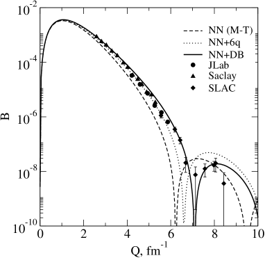
Figure 7: The structure function $B(Q)$ of elastic e-d scattering. The impulse approximation (IA) result for the Moscow-Tuebingen potential model kuk1 is shown by the dashed line. The sum of IA and the diagonal ($s^{6}\to s^{6}$) and non-diagonal ($s^{6}\to s^{4}p^{2}$) bare 6q-contributions is shown by the dotted line. The total contribution of the IA+ bare dibaryon + DB (contact term) contribution is represented by the solid line. The data are taken from sac (Saclay), slac (SLAC) and jlab (JLab).

In the model developed here, the contact term which is tightly related to the intermediate dibaryon production has just the necessary properties. Adding the contribution of the DB contact term (51) in line with Eq. (50) results immediately in very good description for the deuteron magnetic form factor $B(Q^{2})$ as shown by the solid line in Fig. 7. Thus, a rather minor renormalization of the $DB$ contact term by a factor of 0.7 makes it possible to describe quantitatively both the deuteron magnetic moment $\mu$ and the behavior of $B(Q^{2})$ in the large momentum transfer region $Q^{2}\lesssim$ 2,5 GeV²/c². Finally, by fixing this minor renormalization of the contact term the calculation the circular polarization $P_{\gamma}$ will be parameter-free.

VI.2 The circular polarization of photons in reaction $\vec{n}+p\to d+\vec{\gamma}$

The contribution of the dibaryon current to the isoscalar $M1$ transition ${}^{3}S_{1}(NN)\to^{3}S_{1}(d)$ is calculated now in the same way. When the spin-dependent operator (49) in the matrix element (36) is replaced by the contact term (26) the $M1$-transition amplitude for the circularly polarized $\gamma$-quanta emission is obtained as

$$\Delta M1^{(\lambda)}_{MM^{\prime}}=Z\int d^{3}r^{\prime}\int d^{3}r\,\Psi^{d}_{M^{\prime}}(\vec{r}^{\,\prime})\frac{e}{2M_{N}}i\left[\frac{{\hbox{$\sigma$}\hbox to0.0pt{\hss\hbox{$\sigma$}\hskip 0.39993pt}\hbox to0.0pt{\hss\lower 0.17218pt\hbox{\hbox{$\sigma$}\hbox to0.0pt{\hss\hbox{$\sigma$}\hskip 0.39993pt}}}}_{p}+{\hbox{$\sigma$}\hbox to0.0pt{\hss\hbox{$\sigma$}\hskip 0.39993pt}\hbox to0.0pt{\hss\lower 0.17218pt\hbox{\hbox{$\sigma$}\hbox to0.0pt{\hss\hbox{$\sigma$}\hskip 0.39993pt}}}}_{n}}{2}\times{\bf q}\right]\cdot{\hbox{$\epsilon$}\hbox to0.0pt{\hss\hbox{$\epsilon$}\hskip 0.39993pt}\hbox to0.0pt{\hss\lower 0.17218pt\hbox{\hbox{$\epsilon$}\hbox to0.0pt{\hss\hbox{$\epsilon$}\hskip 0.39993pt}}}}^{(\lambda)*}G^{S}_{M}(q^{2})\\ \times\left\{\frac{1}{q}j_{1}(\frac{qr}{2})\frac{d\varphi_{2S}(r)}{dr}\frac{\lambda(E_{d})}{2M_{N}}\varphi_{2S}(r^{\prime})+\varphi_{2S}(r)\frac{\lambda(\varepsilon_{\scriptscriptstyle T})}{2M_{N}}\frac{1}{q}j_{1}(\frac{qr^{\prime}}{2})\frac{d\varphi_{2S}(r^{\prime})}{dr^{\prime}}\right\}\Psi^{np}_{M}(\vec{r},\vec{p}_{n}),$$ (56)

When calculating $P_{\gamma}$ this amplitude must be added to the single-nucleon current terms (42) using the same renormalization constant $Z=$ 0.7. Similarly to the single-nucleon current, the integral (56) is calculated straight-forward by replacement of $j_{1}(qr/2)/q\to r/6$ by $q=E_{d}$. Also we substitute $E=$ 0 instead of $E=\varepsilon_{T}$ and $E=E_{d}$ in the $\lambda(E)$ function in Eq. (2). After this we get for the dibaryon induced current contribution an expression analogous to Eq. (74) with the respective “reduced” dibaryon matrix elements. The amplitude (56) found by this way together with the single-nucleon matrix elements (42) should be included to the final expression for $P_{\gamma}$

$$P^{tot}_{\gamma}=2Re\left\{\frac{M1_{0}}{M1_{1}}+\frac{\Delta M1}{M1_{1}}+\frac{E2_{0}}{M1_{1}}\right\},$$ (57)

where the dibaryon induced current contribution is

$$P_{\gamma}(DB)=2Re\left\{\frac{\Delta M1}{M1_{1}}\right\}.$$ (58)

The results of the numerical calculations within our model are presented in Table 2 together with a parallel calculation for $P_{\gamma}$ with the conventional RSC $NN$-potential model in its modern version RSC93 e . Evidently the fully parameter free prediction of our dibaryon model for $P_{\gamma}$ is in a first time in very good agreement with the respective experimental result.

Table 2: Circular polarization of $\gamma$ quanta in the $\vec{n}+p\to d+\vec{\gamma}$ reaction

	$P_{\gamma}(M1)$	$P_{\gamma}(E2)$	$P_{\gamma}(NN)$	$P_{\gamma}(DB)$	$P^{tot}_{\gamma}$
Model	$\cdot 10^{-3}$	$\cdot 10^{-3}$	$\cdot 10^{-3}$	$\cdot 10^{-3}$	$\cdot 10^{-3}$
Reid 93	-1.761	0.699	-1.062	0.	-1.062
Moscow-Tuebingen	-1.791	0.657	-1.134	-0.261	-1.395
Experiment lob					-1.5$\pm$0.3

VII Short discussion and conclusion

In this paper we developed a model for the new electromagnetic current in the deuteron and in the $NN$ system in general. The new currents are based on the picture of short-range $NN$ interaction via an intermediate dibaryon generation. The dibaryon represents a new degree of freedom and according to a general principle of quantum theory this must inevitably lead to the respective new current(s). By applying the general recipe of minimal substitution to the Hamiltonian of the dibaryon model to derive the new current one gets automatically two different contributions: diagonal and transitional ones. The diagonal current is associated mainly with the quark degrees of freedom, and thus is proportional to the (small) weight of the dibaryon component in the deuteron. While the transitional current leads to a larger contribution to the deuteron electromagnetic properties, and likely also $NN$ electromagnetic observables, especially of isoscalar nature. We studied three such electromagnetic characteristics:

• the magnetic moment $\mu_{d}$ of the deuteron;

• the magnetic form factor $B(Q^{2})$ in the region of its diffraction minimum;

• the circular polarization $P_{\gamma}$ of $\gamma$ quanta in radiative capture of spin-polarized neutrons by hydrogen.

As for the prediction of the deuteron magnetic moment, the new isoscalar dibaryon current just fills perfectly the small gap which was found earlier ($\Delta\mu\simeq$ 0.010 n.m.) between prediction of the dibaryon $NN$-force model and experimental data (see Table 1). With this tiny correction the theoretical deuteron magnetic moment $\mu_{d}$ agrees excellently with its respective experimental value.

In the present study we found that the minimal (gauge) substitution to the dibaryon Hamiltonian gives a strong positive contribution to the $B(Q^{2})$ behavior near the minimum region. Moreover, the parameter-free calculation of the $B(Q^{2})$ in the new model gave already a very reasonable description for the deuteron magnetic form factor $B(Q^{2})$. A minor reduction of the dibaryon-$\gamma$ vertex by a factor 0.7 results in an excellent agreement with the data both for $\mu_{d}$ and $B(Q^{2})$.

After fixing all parameters of the new model, we calculated the magnitude of the circular polarization of photons in $\vec{n}+p\to d+\gamma$ capture at thermal energy. This fully parameter-free calculation gave a result which is in a very close agreement with the existing experimental data lob . It is important to remind the reader that many attempts were undertaken in the past; see e.g. the review of M. Rho rho4 where one can find the references to earlier works and a good discussion of all difficulties encountered in theoretical predictions of $P_{\gamma}$. Thus, this longstanding $P_{\gamma}$-puzzle seems now to be solved.

Here it is useful to discuss briefly the comparison between the present model predictions and some other current models, both microscopic and phenomenological ones. Very detailed six-quark microscopic calculations in Ref. buch have revealed that the quark exchange currents cannot give any quantitative agreement with deuteron data neither for the magnetic nor for the charge form factors, $B(Q^{2})$ and $A(Q^{2})$, respectively. Moreover, when calculating the quark-exchange current corrections to the magnetic and quadrupole deuteron moments the authors buch have found some (although small) underestimation for $\mu_{d}$ but strong overestimation for $Q_{d}$. These disagreements with the respective experimental results have demonstrated that the incorporation of a bare six-quark contribution only cannot fill the gap between the impulse approximation (plus the traditional MEC) results and the experiment, at least for the $M1$- and $E2$-isoscalar transitions. On the other hand, the dressing procedure for six-quark bag has been shown in the present work to lead inevitably to new short-range currents. These dibaryon induced currents should replace the conventional two-body meson-exchange currents at short $NN$-distances when two interacting nucleons are overlapping strongly in which case their meson clouds will fuse into one common cloud of a dibaryon.

The new dibaryon currents proposed and studied in this paper must contribute also to many other electromagnetic properties which could not be explained with the conventional $NN$-models before, e.g. the $\gamma$-induced polarization of nucleons at photo-disintegration of deuteron at low energies, $d(\gamma,\vec{n})p$, and also the electro-disintegration of deuteron, $d(e,e^{\prime}p)n$ at high momentum transfer strok . The particular interest for the new isoscalar current rests in numerous studies of ($e,e^{\prime}pp$) and $(\gamma,pp)$ processes at intermediate energies. It is worth to remember here that the theoretical interpretation of such processes, measured experimentally at various kinematic conditions, failed to explain the accurate experimental findings (see e.g. Ref. groep ). Very likely these processes include some contribution of two-body isoscalar currents as well.

Simultaneously, any success in such consistent interpretation of the data will support strongly the underlying dibaryon model for the short range $NN$ interaction.

Acknowledgments

The authors appreciate very much the discussions with Profs. S.V. Gerasimov and V.E. Lyubovitskij. We are very thankful to Drs. V.N. Pomerantsev, M.A. Shikhalev and M. Kaskulov for very fruitful discussions and help.

Appendix A Avoiding double-counting

It is worth to add here some important comments about a large difference between “diagonal” and “non-diagonal” (transition) currents in the $NN$ system. It is important that the similar consideration of the $t$-channel two-body currents in the $NN$ system (with replacement quarks by nucleons in Fig. 6) within the framework of a traditional $NN$ model does not lead to new currents because the scalar exchange in the $t$-channel is already included somehow into the $NN$ wavefunction $\Psi_{NN}$, and thus the one-nucleon current matrix element $\langle\Psi_{NN}|J^{\mu}_{N}|\Psi_{NN}\rangle$ also includes among the others the diagrams shown in Fig. 6.

In contrast to this (one-channel) problem, we are dealing here with a two- (or more) channel problem and our non-diagonal current operator $V_{Nq\gamma}$ given in Eq. (24) describes electromagnetic induced transition between two different channels, i.e. between the proper $NN$- and dressed bag components. In such transitions there happens a strong rearrangement of the spin-isospin structure of the total six-quark wavefunction, and thus this transition between two components is associated with the real current of magnetic type, which corresponds to the quark spin (isospin) flip. It can be illustrated clearly by considering a transition $|s^{4}p^{2}[42]_{X}\rangle\rightarrow|s^{6}[6]_{X}\rangle$ even with the same value of the total spin S (and isospin T) in the left (bra) and right (ket) vectors in the current matrix element: $\langle{s^{6}}[6]_{X},ST|V_{Nq\gamma}|s^{4}p^{2}[42]_{X},ST\rangle$. Recall also that the configuration $s^{6}$ in our model is fully absent in the initial and final $NN$ states because of the orthogonality condition (14) and the projector appearing in the $NN$ channel.

Let us assume that the spin and isospin in the initial (and final) $NN$-channel and in the intermediate dibaryon state have the values $S=$ 1 and $T=$ 0, which are associated with the spin and isospin Young tableaux for the six-quark system $[42]_{S}$ and $[3^{2}]_{T}$ respectively. As a result, we get the following transition matrix element

$$\langle s^{6}[6]_{X}[42]_{S}[3^{2}]_{T}([f^{\prime}_{ST}]),[2^{3}]_{C}|\\ \times V_{Nq\gamma}\,|s^{4}p^{2}[42]_{X}[42]_{S}[3^{2}]_{T}([f_{ST}]),[2^{3}]_{C}\rangle$$ (59)

It is important to stress here that $[f^{\prime}_{ST}]\neq[f_{ST}]$, i.e. the spin-isospin structure in bra- and ket states are different, because the Pauli principle severely restricts the form of the spin-isospin tableau $[f^{\prime}_{ST}]$ on the left hand side state reducing it to a single allowable state $[42]_{S}\cdot[3^{2}]_{T}\to[f^{\prime}_{ST}]=[3^{2}]_{ST}$. In contrast to it, on the right hand side state any spin-isospin Young tableau $[42]_{S}\cdot[3^{2}]_{T}\to[f_{ST}]=[51]_{ST}\!+\![41^{2}]_{ST\!}+\![3^{2}]_{ST}\!+\![321]_{ST}\!+\![2^{2}1^{2}]_{ST}$ is permissible (see e.g. Refs. obu0 ).

Therefore even the static magnetic moments for left and right functions must be different. It is worth to remember here that just the spin-isospin Young tableau $[f]_{ST}$ determines fully the nucleon magnetic moment $\mu_{N}$ at $S=$ 1/2 and $T=$ 1/2, and the correct value $\mu_{N}$ both for proton and neutron can be obtained only for the symmetric ST-state $[3]_{ST}$ satisfying the Pauli exclusion principle. Hence, in the transitions (59) we have real currents describing the spin-isospin flip in the $NN\to DB$ transition, and thus, the current operator $V_{Nq\gamma}$ makes a non-trivial (two-body) contribution to the total current in the two-channel system $NN+DB$.

Appendix B Derivation of the contact $NN\Leftrightarrow NN\gamma$ term

In deriving of Eq. (26) we start from Eq. (4) and substitute the vertex $Nq\gamma$ (24) in one of two matrix elements of the $s^{4}p^{2}\to s^{6}$ transition $<s^{4}p^{2}\{f\}|V_{Nq}|s^{6}[6]_{\scriptscriptstyle X}>$ in the r.h.s. of Eq. (4). It gives

$$V_{NqN\gamma}\simeq\sum_{ff^{\prime}}\left[\langle\!NN|s^{4}p^{2}\{f\}\rangle\,\langle s^{4}p^{2}\{f\}|V_{Nq\gamma}|s^{6}\rangle\,G_{DB}\,\langle s^{6}|V_{Nq}|s^{4}p^{2}\{f^{\prime}\}\rangle\,\langle s^{4}p^{2}\{f^{\prime}\}|NN\rangle\right.\\ \left.+\langle NN|s^{4}p^{2}\{f\}\langle\,\rangle s^{4}p^{2}\{f\}|V_{Nq}|s^{6}\rangle\,G_{DB}\,\langle s^{6}|V_{Nq\gamma}|s^{4}p^{2}\{f^{\prime}\}\langle\,\rangle s^{4}p^{2}\{f^{\prime}\}|NN\rangle\right]$$ (60)

(non-significant details are omitted here). The calculation of this operator is performed with the fractional parentage coefficient technique (see Refs. obu1 ; obu0 ; obu2 for details) by factorizing the fixed pair $ij$ of quarks with numbers $i=$ 3 and $j=$ 6. The space coordinates of this pair depend on proton and neutron center-of-mass coordinates, ${\bf r}_{p}$ and ${\bf r}_{n}$ respectively, and on the relative motion Jacobi coordinates ${\hbox{$\rho$}\hbox to0.0pt{\hss\hbox{$\rho$}\hskip 0.39993pt}\hbox to0.0pt{\hss\lower 0.17218pt\hbox{\hbox{$\rho$}\hbox to0.0pt{\hss\hbox{$\rho$}\hskip 0.39993pt}}}}_{p1}$, ${\hbox{$\rho$}\hbox to0.0pt{\hss\hbox{$\rho$}\hskip 0.39993pt}\hbox to0.0pt{\hss\lower 0.17218pt\hbox{\hbox{$\rho$}\hbox to0.0pt{\hss\hbox{$\rho$}\hskip 0.39993pt}}}}_{p2}$, $\hbox{$\rho$}\hbox to0.0pt{\hss\hbox{$\rho$}\hskip 0.39993pt}\hbox to0.0pt{\hss\lower 0.17218pt\hbox{\hbox{$\rho$}\hbox to0.0pt{\hss\hbox{$\rho$}\hskip 0.39993pt}}}_{n1}$ and ${\hbox{$\rho$}\hbox to0.0pt{\hss\hbox{$\rho$}\hskip 0.39993pt}\hbox to0.0pt{\hss\lower 0.17218pt\hbox{\hbox{$\rho$}\hbox to0.0pt{\hss\hbox{$\rho$}\hskip 0.39993pt}}}}_{n2}$, as defined in Eq. (6) and below

$${\bf r}_{3}={\bf R}+{\bf r}_{p}-2{\hbox{$\rho$}\hbox to0.0pt{\hss\hbox{$\rho$}\hskip 0.39993pt}\hbox to0.0pt{\hss\lower 0.17218pt\hbox{\hbox{$\rho$}\hbox to0.0pt{\hss\hbox{$\rho$}\hskip 0.39993pt}}}}_{p2}/3,\quad{\bf r}_{6}={\bf R}+{\bf r}_{n}-2{\hbox{$\rho$}\hbox to0.0pt{\hss\hbox{$\rho$}\hskip 0.39993pt}\hbox to0.0pt{\hss\lower 0.17218pt\hbox{\hbox{$\rho$}\hbox to0.0pt{\hss\hbox{$\rho$}\hskip 0.39993pt}}}}_{n2}/3,\\ {\bf R}=\frac{1}{6}\sum_{i\!=\!1}^{6}{\bf r}_{i}.$$ (61)

In the c.m. frame ${\bf R}=$ 0 and ${\bf r}_{p}=-{\bf r}_{n}={\bf r}/2$. The conjugated momenta ${\bf p}_{3}$ and ${\bf p}_{6}$ reads

$${\bf p}_{3}={\bf P}+2({\bf p}_{p}-{\bf p}_{n})/3-{\hbox{$\pi$}\hbox to0.0pt{\hss\hbox{$\pi$}\hskip 0.39993pt}\hbox to0.0pt{\hss\lower 0.17218pt\hbox{\hbox{$\pi$}\hbox to0.0pt{\hss\hbox{$\pi$}\hskip 0.39993pt}}}}_{p2},\\ {\bf p}_{6}={\bf P}-2({\bf p}_{p}-{\bf p}_{n})/3-{\hbox{$\pi$}\hbox to0.0pt{\hss\hbox{$\pi$}\hskip 0.39993pt}\hbox to0.0pt{\hss\lower 0.17218pt\hbox{\hbox{$\pi$}\hbox to0.0pt{\hss\hbox{$\pi$}\hskip 0.39993pt}}}}_{n2},$$ (62)

where ${\hbox{$\pi$}\hbox to0.0pt{\hss\hbox{$\pi$}\hskip 0.39993pt}\hbox to0.0pt{\hss\lower 0.17218pt\hbox{\hbox{$\pi$}\hbox to0.0pt{\hss\hbox{$\pi$}\hskip 0.39993pt}}}}_{p2}$ and ${\hbox{$\pi$}\hbox to0.0pt{\hss\hbox{$\pi$}\hskip 0.39993pt}\hbox to0.0pt{\hss\lower 0.17218pt\hbox{\hbox{$\pi$}\hbox to0.0pt{\hss\hbox{$\pi$}\hskip 0.39993pt}}}}_{n2}$ are the relative momenta conjugated to ${\hbox{$\rho$}\hbox to0.0pt{\hss\hbox{$\rho$}\hskip 0.39993pt}\hbox to0.0pt{\hss\lower 0.17218pt\hbox{\hbox{$\rho$}\hbox to0.0pt{\hss\hbox{$\rho$}\hskip 0.39993pt}}}}_{p2}$ and ${\hbox{$\rho$}\hbox to0.0pt{\hss\hbox{$\rho$}\hskip 0.39993pt}\hbox to0.0pt{\hss\lower 0.17218pt\hbox{\hbox{$\rho$}\hbox to0.0pt{\hss\hbox{$\rho$}\hskip 0.39993pt}}}}_{n2}$ respectively, ${\bf P}=\sum_{i\!=\!1}^{6}{\bf p}_{i}$.

The calculation of the Fourier transform $\int\frac{d^{3}p_{1}}{(2\pi)^{3}}\dots\int\frac{d^{3}p_{6}}{(2\pi)^{3}}exp(i{\bf p}_{1}\cdot{\bf r}_{1}+\dots+i{\bf p}_{6}\cdot{\bf r}_{6})$ for the matrix elements of operators $V_{Nq\gamma}$ and $V_{Nq}$ on the r.h.s. of Eq. (60) and substitution of the integral $\int exp\{-i({\bf p}_{3}+{\bf p}_{6}-{\bf p}^{\prime}_{3}-{\bf p}^{\prime}_{6}-{\bf q})\cdot{\bf x}\}d{\bf x}$ for the $\delta$-function $(2\pi)^{3}\delta^{3}({\bf p}_{3}+{\bf p}_{6}-{\bf p}^{\prime}_{3}-{\bf p}^{\prime}_{6}-{\bf q})$ lead, after the simple but tedious mathematics, to the following expression for the $r$-dependent part of the $NN\to DB+\gamma$ vertex in Eq. (60)

$$\tilde{V}_{Nq\gamma}(q,r)=\frac{e}{2M_{\scriptscriptstyle N}}F_{\scriptscriptstyle N}({\bf q}^{2})\,g_{s}^{2}\,\langle v\rangle\,\left\{e^{-i{\bf q}\cdot{\bf r}/2}\mu_{p}\frac{1}{M_{\scriptscriptstyle N}}{\hbox{$\nabla$}\hbox to0.0pt{\hss\hbox{$\nabla$}\hskip 0.39993pt}\hbox to0.0pt{\hss\lower 0.17218pt\hbox{\hbox{$\nabla$}\hbox to0.0pt{\hss\hbox{$\nabla$}\hskip 0.39993pt}}}}_{r}\cdot[{\hbox{$\epsilon$}\hbox to0.0pt{\hss\hbox{$\epsilon$}\hskip 0.39993pt}\hbox to0.0pt{\hss\lower 0.17218pt\hbox{\hbox{$\epsilon$}\hbox to0.0pt{\hss\hbox{$\epsilon$}\hskip 0.39993pt}}}}^{(\lambda)}\times{\hbox{$\sigma$}\hbox to0.0pt{\hss\hbox{$\sigma$}\hskip 0.39993pt}\hbox to0.0pt{\hss\lower 0.17218pt\hbox{\hbox{$\sigma$}\hbox to0.0pt{\hss\hbox{$\sigma$}\hskip 0.39993pt}}}}_{p}]-e^{i{\bf q}\cdot{\bf r}/2}\mu_{n}\frac{1}{M_{\scriptscriptstyle N}}{\hbox{$\nabla$}\hbox to0.0pt{\hss\hbox{$\nabla$}\hskip 0.39993pt}\hbox to0.0pt{\hss\lower 0.17218pt\hbox{\hbox{$\nabla$}\hbox to0.0pt{\hss\hbox{$\nabla$}\hskip 0.39993pt}}}}_{r}\cdot[{\hbox{$\epsilon$}\hbox to0.0pt{\hss\hbox{$\epsilon$}\hskip 0.39993pt}\hbox to0.0pt{\hss\lower 0.17218pt\hbox{\hbox{$\epsilon$}\hbox to0.0pt{\hss\hbox{$\epsilon$}\hskip 0.39993pt}}}}^{(\lambda)}\times{\hbox{$\sigma$}\hbox to0.0pt{\hss\hbox{$\sigma$}\hskip 0.39993pt}\hbox to0.0pt{\hss\lower 0.17218pt\hbox{\hbox{$\sigma$}\hbox to0.0pt{\hss\hbox{$\sigma$}\hskip 0.39993pt}}}}_{n}]\right\}\varphi_{2S}(r).$$ (63)

The terms with factors $\frac{\hat{\bf q}\cdot{\bf k}_{i}}{m_{q}}[{\hbox{$\sigma$}\hbox to0.0pt{\hss\hbox{$\sigma$}\hskip 0.39993pt}\hbox to0.0pt{\hss\lower 0.17218pt\hbox{\hbox{$\sigma$}\hbox to0.0pt{\hss\hbox{$\sigma$}\hskip 0.39993pt}}}}_{i}\times\hat{\bf q}]$ on the r.h.s. of Eq. (24) are canceled after the summation in the Eq. (60). Now the expression (63) should replace the function $\varphi(r)\varphi_{2S}(r)$ in the separable potential (1) in line with the interpretation of the vertex matrix element in Eq. (7).

In Eq. (63) we use the standard formulas of CQM for the nucleon form factor

$$F_{\scriptscriptstyle N}({\bf q}^{2})=F_{q}(q^{2})\int|\psi_{N}(\rho_{1},\rho_{2}))|^{2}e^{i2{\hbox{$\rho$}\hbox to0.0pt{\hss\hbox{$\rho$}\hskip 0.27995pt}\hbox to0.0pt{\hss\lower 0.12053pt\hbox{\hbox{$\rho$}\hbox to0.0pt{\hss\hbox{$\rho$}\hskip 0.27995pt}}}}_{2}\cdot{\bf q}/3}d^{3}\rho_{1}d^{3}\rho_{2}$$ (64)

and for the magnetic momentum of nucleon

$$\langle N(3q),[21]_{\scriptscriptstyle S}[21]_{\scriptscriptstyle T}:[3]_{\scriptscriptstyle ST}|\\ \times\sum_{i\!=\!1}^{3}\frac{\hat{e}_{i}{\hbox{$\sigma$}\hbox to0.0pt{\hss\hbox{$\sigma$}\hskip 0.39993pt}\hbox to0.0pt{\hss\lower 0.17218pt\hbox{\hbox{$\sigma$}\hbox to0.0pt{\hss\hbox{$\sigma$}\hskip 0.39993pt}}}}_{i}}{2m_{q}}|N(3q),[21]_{\scriptscriptstyle S}[21]_{\scriptscriptstyle T}:[3]_{\scriptscriptstyle ST}\rangle\,=\,\frac{\mu_{\scriptscriptstyle N}{\hbox{$\sigma$}\hbox to0.0pt{\hss\hbox{$\sigma$}\hskip 0.39993pt}\hbox to0.0pt{\hss\lower 0.17218pt\hbox{\hbox{$\sigma$}\hbox to0.0pt{\hss\hbox{$\sigma$}\hskip 0.39993pt}}}}_{\scriptscriptstyle N}}{2M_{\scriptscriptstyle N}},$$ (65)

$N\!=\!n,p$, with $\mu_{p}=$ 3, $\mu_{n}=$ -2. The gradients in Eq. (63) originate from the proton and neutron momenta ${\bf k}_{p}$ and ${\bf k}_{n}$ which appear in the momentum representation of the vertex (63) as a result of substitution of Eqs. (62) for the quark momenta ${\bf p}_{3}$ and ${\bf p}_{6}$. In the coordinate representation, these momenta transform into gradients $-i{\hbox{$\nabla$}\hbox to0.0pt{\hss\hbox{$\nabla$}\hskip 0.39993pt}\hbox to0.0pt{\hss\lower 0.17218pt\hbox{\hbox{$\nabla$}\hbox to0.0pt{\hss\hbox{$\nabla$}\hskip 0.39993pt}}}}_{r_{p}}=-i{\hbox{$\nabla$}\hbox to0.0pt{\hss\hbox{$\nabla$}\hskip 0.39993pt}\hbox to0.0pt{\hss\lower 0.17218pt\hbox{\hbox{$\nabla$}\hbox to0.0pt{\hss\hbox{$\nabla$}\hskip 0.39993pt}}}}_{r/2}$ and $-i{\hbox{$\nabla$}\hbox to0.0pt{\hss\hbox{$\nabla$}\hskip 0.39993pt}\hbox to0.0pt{\hss\lower 0.17218pt\hbox{\hbox{$\nabla$}\hbox to0.0pt{\hss\hbox{$\nabla$}\hskip 0.39993pt}}}}_{r_{n}}=i{\hbox{$\nabla$}\hbox to0.0pt{\hss\hbox{$\nabla$}\hskip 0.39993pt}\hbox to0.0pt{\hss\lower 0.17218pt\hbox{\hbox{$\nabla$}\hbox to0.0pt{\hss\hbox{$\nabla$}\hskip 0.39993pt}}}}_{r/2}$ respectively. The nucleon mass $M_{\scriptscriptstyle N}$ in Eq. (65) is a result of the substitution of $M_{\scriptscriptstyle N}$ for the value 3$m_{q}$ which appears in the r.h.s. of Eq. (60) resulting from CQM algebra.

Making use of the expressions

$${\hbox{$\nabla$}\hbox to0.0pt{\hss\hbox{$\nabla$}\hskip 0.39993pt}\hbox to0.0pt{\hss\lower 0.17218pt\hbox{\hbox{$\nabla$}\hbox to0.0pt{\hss\hbox{$\nabla$}\hskip 0.39993pt}}}}_{r}\varphi_{2S}(r)=\hat{\bf r}\frac{d}{dr}\varphi_{2S}(r),\qquad e^{\pm i{\bf q}\cdot{\bf r}/2}=\\ j_{0}(qr/2)\pm i\sqrt{4\pi}j_{1}(qr/2)\sum_{m}Y_{1m}(\hat{q})Y_{1m}^{*}(\hat{r})+\dots,$$ (66)

and adding the contributions of two graphs ($a$) and ($b$) depicted in Fig. 4 we obtain finally Eq. (26) for the $NqN\gamma$ (contact) term.

Appendix C Nucleon and dibaryon electromagnetic matrix elements

The general formula for the nucleon electromagnetic current

$$eJ_{\scriptscriptstyle N}^{\mu}=e_{\scriptscriptstyle N}\gamma^{\mu}F_{1}^{\scriptscriptstyle N}(q^{2})+i\frac{e\mu_{\scriptscriptstyle N}-e_{\scriptscriptstyle N}}{2M_{\scriptscriptstyle N}}\sigma^{\mu\nu}q^{\nu}F_{2}^{\scriptscriptstyle N}(q^{2}),\\ e_{\scriptscriptstyle N}=e(\frac{1}{2}+\frac{\tau_{z}}{2})$$ (67)

can easily be derived after averaging the quark current (22) over the nucleon wavefunction:

$$eJ_{{\scriptscriptstyle N}QM}^{\mu}=\langle N(123)|\sum_{i\!=\!1}^{3}j^{\mu}_{i}(q)|N(123)\rangle\\ =\left[e_{\scriptscriptstyle N}\gamma^{\mu}+i\frac{e\mu_{\scriptscriptstyle NQM}-e_{\scriptscriptstyle N}}{2M_{\scriptscriptstyle N}}\sigma^{\mu\nu}q^{\nu}\right]F_{QM}(q^{2}),$$ (68)

in which the quark-model predictions

$$\mu_{p{\scriptscriptstyle QM}}=3,\quad\mu_{n{\scriptscriptstyle QM}}=-2,\\ F_{QM}(Q^{2})=F_{q}(Q^{2})e^{-Q^{2}b^{2}/6}$$ (69)

are not distinguished seriously from their experimentally measured counterparts used in Eq. (67):

$$\mu_{p}=2.79,\quad\mu_{n}=-1.91,\\ F_{2}(Q^{2})\approx F_{dip}(Q^{2})=\left(\frac{1}{1+\frac{Q^{2}}{\Lambda_{N}^{2}}}\right)^{2}.$$ (70)

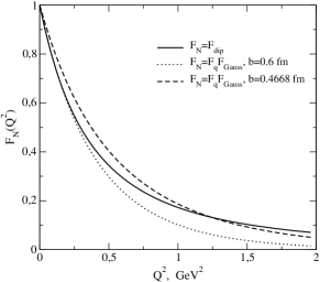
Figure 8: Comparison of the simple quark model description for the nucleon magnetic form factor (with different scale values $b$) with those parametrized through the standard dipole fit.

It is important to stress here that the quark-model magnetic form factor, as can be seen in Fig. 8, resembles quite precisely the respective nucleon form factor found with the standard dipole fit, in the region $Q^{2}\simeq$ 1 - 2 GeV²/c², i.e. near the region of minimum for the deuteron magnetic form factor $B(Q^{2})$ — see the respective curve in Fig. 8 for the choice of $b=\sqrt{\frac{3}{2}}r_{0}\simeq$ 0.47 fm.

Thus, in the nucleon sector, we replace the quark-model current $J_{{\scriptscriptstyle N}QM}^{\mu}$ with the standard representation of the nucleon current $J_{{\scriptscriptstyle N}}^{\mu}$ given by Eqs. (67) and (70), and the non-additive two-body current (which gives only a small correction to the single-nucleon current $J_{{\scriptscriptstyle N}}^{\mu}$) only is calculated on the basis of the constituent quark model (CQM).

In particular, the CQM technique is used for calculation of the last two terms in Eq. (27). These terms are contributions of the graphs shown in Figs. 5(f) and (e) respectively.

• For the graph in Fig. 5(f), the diagonal matrix element $\langle DB|\sum_{i\!=\!1}^{6}j^{\mu}_{i}\varepsilon_{\mu}^{(\lambda)}|DB\rangle$ is reduced here to the matrix element with the $s^{6}$ bag-like wavefunctions. This term is found by the same technique as for the nucleon matrix element calculation in Eqs. (68) and (69). As a result, for the transverse current component ($\lambda=\pm$ 1, $\varepsilon_{\mu}^{(\lambda)}=\{0,{\hbox{$\epsilon$}\hbox to0.0pt{\hss\hbox{$\epsilon$}\hskip 0.39993pt}\hbox to0.0pt{\hss\lower 0.17218pt\hbox{\hbox{$\epsilon$}\hbox to0.0pt{\hss\hbox{$\epsilon$}\hskip 0.39993pt}}}}^{(\lambda)}\}$) one gets

  $$\langle DB|\sum_{i\!=\!1}^{6}j^{\mu}_{i}\varepsilon_{\mu}^{(\lambda)}|DB\rangle=\\ \langle s^{6},S\!=\!1,\,T\!=\!0\,|\sum_{i\!=\!1}^{6}j^{\mu}_{i}\varepsilon_{\mu}^{(\lambda)}\,|\,s^{6},S\!=\!1,\,T\!=\!0\rangle\\ =\,-\,\frac{({\hbox{$\sigma$}\hbox to0.0pt{\hss\hbox{$\sigma$}\hskip 0.39993pt}\hbox to0.0pt{\hss\lower 0.17218pt\hbox{\hbox{$\sigma$}\hbox to0.0pt{\hss\hbox{$\sigma$}\hskip 0.39993pt}}}}_{p}\!+\!{\hbox{$\sigma$}\hbox to0.0pt{\hss\hbox{$\sigma$}\hskip 0.39993pt}\hbox to0.0pt{\hss\lower 0.17218pt\hbox{\hbox{$\sigma$}\hbox to0.0pt{\hss\hbox{$\sigma$}\hskip 0.39993pt}}}}_{n})\cdot{\hbox{$\epsilon$}\hbox to0.0pt{\hss\hbox{$\epsilon$}\hskip 0.39993pt}\hbox to0.0pt{\hss\lower 0.17218pt\hbox{\hbox{$\epsilon$}\hbox to0.0pt{\hss\hbox{$\epsilon$}\hskip 0.39993pt}}}}^{(\lambda)}}{2}\mu_{\scriptscriptstyle N}^{s}F_{s^{6}}(Q^{2}),$$ (71)

  with $F_{s^{6}}(Q^{2})=F_{q}(Q^{2})e^{-5Q^{2}b^{2}/24},\quad\mu_{\scriptscriptstyle N}^{s}=\mu_{p}+\mu_{n}$.

• With the graph in Fig. 5(e), the transition matrix element $NN\to DB$ can be found similarly to Eq. (4), i.e. by using the expansion over the six-quark shell-model states with restriction by the most important low-lying states

$$\langle d(NN)|\sum_{i\!=\!1}^{6}j^{\mu}_{i}\varepsilon_{\mu}^{(\lambda)}|DB\rangle\,=\sum_{f}\int u(r)\langle N(123)|\langle N(456)|\,s^{4}p^{2}\{f\}\rangle dr\,\langle s^{4}p^{2}\{f\}\,|\sum_{i\!=\!1}^{6}j^{\mu}_{i}\varepsilon_{\mu}^{(\lambda)}|\,s^{6}\rangle\\ =\,-\,\frac{({\hbox{$\sigma$}\hbox to0.0pt{\hss\hbox{$\sigma$}\hskip 0.39993pt}\hbox to0.0pt{\hss\lower 0.17218pt\hbox{\hbox{$\sigma$}\hbox to0.0pt{\hss\hbox{$\sigma$}\hskip 0.39993pt}}}}_{p}\!+\!{\hbox{$\sigma$}\hbox to0.0pt{\hss\hbox{$\sigma$}\hskip 0.39993pt}\hbox to0.0pt{\hss\lower 0.17218pt\hbox{\hbox{$\sigma$}\hbox to0.0pt{\hss\hbox{$\sigma$}\hskip 0.39993pt}}}}_{n})\cdot{\hbox{$\epsilon$}\hbox to0.0pt{\hss\hbox{$\epsilon$}\hskip 0.39993pt}\hbox to0.0pt{\hss\lower 0.17218pt\hbox{\hbox{$\epsilon$}\hbox to0.0pt{\hss\hbox{$\epsilon$}\hskip 0.39993pt}}}}^{(\lambda)}}{2}\langle u|2S(NN)\rangle\sum_{f}C_{f}F_{s^{6}-s^{4}p^{2}}(Q^{2}).$$ (72)

Here $F_{s^{6}-s^{4}p^{2}}(Q^{2})=\frac{5Q^{2}b^{2}}{24}e^{-5Q^{2}b^{2}/24}$ and $<u|2S(NN)>=\int_{0}^{\infty}u(r)\varphi_{2S}(r)dr$.

Appendix D Deuteron $M$1- and $E$2- transition amplitudes

The M1- and E2-amplitudes which are used for the cross section calculation in Eqs. (38) and (39) take the following form (we present here them separately for the spin (s)- and convection (c) current components):

$$M1^{(\lambda)I\!=\!1}_{\scriptscriptstyle MM^{\prime}}(s)=\delta_{\scriptscriptstyle M^{\prime},-\lambda}\delta_{\scriptscriptstyle M,0}\,(\mu_{n}-\mu_{p})\,\lambda\left(\frac{-ieq}{2m_{N}}\right)I_{0}(u,{}^{1}S_{0}),$$ (73)

$$M1^{(\lambda)I\!=\!0}_{\scriptscriptstyle MM^{\prime}}(s)=\delta_{\scriptscriptstyle M^{\prime},M-\lambda}\,(\mu_{n}+\mu_{p})\,[\lambda\sqrt{2}(1M1-\!\lambda)|1(M\!-\!\lambda)]\left(\frac{-ieq}{2m_{N}}\right)\\ \times\left\{I_{0}(u,{}^{3}S_{1})-\frac{1}{2}I_{0}(w,{}^{3}D_{1})+\frac{1}{\sqrt{2}}I_{2}(uw,{{}^{3}S_{1}}{}^{3}D_{1})+\frac{1}{2}I_{2}(w,{}^{3}D_{1})\right\},$$ (74)

$$M1^{(\lambda)I\!=\!0}_{\scriptscriptstyle MM^{\prime}}(c) = \delta_{\scriptscriptstyle M^{\prime},M-\lambda}\,[\lambda\sqrt{2}(1M1-\!\lambda)|1(M\!-\!\lambda)]\left(\frac{-ieq}{2m_{N}}\right)\frac{3}{8}\left\{I_{0}(w,{}^{3}D_{1})+I_{2}(w,{}^{3}D_{1})\right\},$$ (75)

$$E2^{(\lambda)}_{\scriptscriptstyle MM^{\prime}}(s) = \delta_{\scriptscriptstyle M^{\prime},M-\lambda}(\mu_{n}+\mu_{p})\left[-\frac{\sqrt{10}}{\sqrt{3}}(1M2-\!\lambda)|1(M\!-\!\lambda)\right]\left(\frac{-ieq}{2m_{N}}\right)\frac{3}{\sqrt{2}}I_{2}(uw,{{}^{3}S_{1}}{}^{3}D_{1}),$$ (76)

$$E2^{(\lambda)}_{\scriptscriptstyle MM^{\prime}}(c) = \delta_{\scriptscriptstyle M^{\prime},M-\lambda}\,[\lambda\sqrt{2}(1M1-\!\lambda)|1(M\!-\!\lambda)]\left(\frac{-ieq}{2m_{N}}\right)\frac{3}{8}\left\{I_{0}(w,{}^{3}D_{1})+I_{2}(w,{}^{3}D_{1})\right\},$$ (77)

where $I_{0}$ and $I_{2}$ are the following overlap integrals

$$I_{0}(f,Z)=\int_{0}^{\infty}f(r)Z(r,p_{n})j_{0}(qr/2)dr,\qquad I_{2}(f,Z)=\int_{0}^{\infty}f(r)Z(r,p_{n})j_{2}(qr/2)dr,$$

$$I_{2}(uw,{{}^{3}S_{1}}{}^{3}D_{1})=\frac{1}{2}\int_{0}^{\infty}\left[u(r){}^{3}D_{1}(r,p_{n})+w(r){}^{3}S_{1}(r,p_{n})\right]j_{2}(qr/2)dr.$$ (78)

Here $Z(r,p_{n})$ can be any of the scattering wavefunctions in ${}^{1}S_{0}$, ${}^{3}S_{1}$ or ${}^{3}D_{1}$ channels.

For the sake of convenience, the factors which are equal to unity on modulo are separated out in square brackets:

$$\lambda\sqrt{2}(1M1-\!\lambda)|1(M\!-\!\lambda)=1,\qquad-\frac{\sqrt{10}}{\sqrt{3}}(1M2-\!\lambda)|1(M\!-\!\lambda)=(-1)^{M}.$$

When summing over the $M$ and $\lambda$ induces, these terms play a role similar to the Kroneker delta.

References

• (1) A. Bazhenov et al, Phys.Lett. B 289, 17 (1992): V.A. Vesna, E.A. Kolomensky, V.P. Kopeliovich, V.M. Lobashev, V.A. Nazarenko, A.N. Pirozhkov, and E.V. Shulgina, Nucl. Phys. A352, 181 (1981).
• (2) T.M. Müller et al, In: Proceedings of the “International Workshop on Particle Physics with Slow Neutrons”, ILL, Grenoble, France, 1998
• (3) S. Aufret et al., Phys. Rev. Lett. 54, 649 (1985).
• (4) R.G. Arnold et al., Phys. Rev. Lett. 58, 1723 (1987).
• (5) D. Abbot et al.,Phys. Rev. Lett. 82, 1379 (1999).
• (6) D.R. Phillips, S.J. Wallace, and N.K. Divin, Phys. Rev. C72, 014006 (2005).
• (7) E. Hammel and J.A. Tjon, Phys. Rev. Lett. 63, 1788 (1989); Phys. Rev. C42, 423 (1990); C49, 21 (1994).
• (8) R. Schiavilla, Phys. Rev. C72, 034001 (2005).
• (9) W.P. Sitarski, P.O Blunden and E.L. Lomon, Phys. Rev. C36, 2479 (1987).
• (10) H. Arenhövel, F. Ritz, and T. Wilbois, Phys. Rev. C61, 034002 (2000).
• (11) J. Carlson and R. Schiavilla, Rev. Mod. Phys. 70, 743 (1998).
• (12) D.O. Riska, Phys. Scr. 31, 471 (1985); Phys. Rep. 181, 207 (1989).
• (13) L.E. Marcucci et al, Phys. Rev. C72, 014001 (2005).
• (14) T-S. Park, K. Kubodera, D-P. Min, and M. Rho, arXiv:nucl-th/9904053 (1999).
• (15) J.-W. Chen, G. Rupak and M.J. Savage, Phys.Lett. B 464, 1 (1999).
• (16) G. Breit and M.L. Rustgi, Nucl. Phys. A161, 337 (1971).
• (17) K. Kubodera, J. Delorm, M. Rho, Phys.Rev.Lett. 40, 755 (1978).
• (18) T.-S. Park, D.-P. Min and M. Rho, Phys. Rep. 233, 341 (1993); Nucl. Phys. A 515, 139 (1990).
• (19) T.-S. Park, D.-P. Min and M.Rho, Phys. Rev. Lett. 74, 4153 (1995); Nucl. Phys. A 596, 515 (1996).
• (20) T. Sasakava and S. Ishikawa, Few-Body Syst. 1, 3 (1986).
• (21) A.P. Burichenko and I.B. Khriplovich, Nucl. Phys. A515, 139 (1990).
• (22) V.I. Kukulin, I.T. Obukhovsky, V.N. Pomerantsev, and A. Faessler, J.Phys. G: Nucl. Part. Phys. 27, 1851 (2001).
• (23) V.I. Kukulin, I.T. Obukhovsky, V.N. Pomerantsev, and A. Faessler, Int. J. Mod. Phys. E 11, 1 (2002).
• (24) V.I. Kukulin and M.A. Shikhalev, Phys. At. Nucl. 67, 1558 (2004).
• (25) A. Faessler, V.I. Kukulin, and M.A. Shikhalev, Ann. Phys. (NY) 320, 71 (2005).
• (26) Y. Yamauchi and M. Wakamatsu, Nucl. Phys. A457, 621 (1986).
• (27) M. Oka and K. Yazaki, Nucl. Phys. A402, 477 (1983).
• (28) E.M. Henley, L.S. Kisslinger, and G.A. Miller, Phys. Rev. C28, 1277 (1983); K. Bräuer, E. Henley, and G.A. Miller, Phys. Rev. C34, 1779 (1986)
• (29) A. Buchmann, Y. Yamauchi, and A. Faessler, Nucl. Phys. A496, 621 (1989).
• (30) A.P. Kobushkin, Yad. Fiz. 62, 1213 (1999).
• (31) F. Wang et al., Phys. Rev. C51, 3411 (1995).
• (32) H.R. Pang, J.L. Ping, F. Wang, T. Goldman, and E.G. Zhao, Phys. Rev. C69, 065207 (2004); nucl-th/0306043.
• (33) T. Goldman, Phys. Rev. C39, 1889 (1989).
• (34) H. Pang et al., Phys. Rev. C70, 035201 (2004).
• (35) S.-i. Ardo and C.H. Hyun, Phys. Rev. C72, 014008 (2005).
• (36) S.R. Beane, P.F. Bedaque, M.J. Savage, and U. van Kolk, Nucl. Phys. A700, 377 (2002).
• (37) S. Fleming, T. Mehen, and I.W. Stewart, Nucl. Phys. A677, 313 (2002).
• (38) A.S. Khrykin et al., Phys. Rev. C69, 034001 (2004).
• (39) A.S. Khrykin, Nucl. Phys. A721, 625c (2003); nucl-exp/0211034.
• (40) P.A, Zolnierczuk et al., Phys. Lett. B549, 301 (2002); Acta Physika Polonika B31, 2349 (2000).
• (41) V.I. Kukulin, V.N. Pomerantsev, M. Kaskulov, and A. Faessler, J. Phys. G30, 287 (2004); V.I. Kukulin, V.N. Pomerantsev, and A. Faessler, J. Phys. G30, 309 (2004).
• (42) N. Kaiser, R. Brockman, and W. Weise, Nucl. Phys. A625, 758 (1997); N. Kaiser, S. Gerstendorfer, and W. Weise, Nucl. Phys. A637, 395 (1998).
• (43) E. Oset et al., Progr. Theor. Phys. 103, 351 (2000).
• (44) M.M. Kaskulov and H. Clement, Phys. Rev. C70, 014002 (2004).
• (45) O. Krehl, C. Hanhart, S. Krewald, and J. Speth, Phys. Rev. C62, 025207 (2000).
• (46) B. D. Serot and J. D. Walecka, Adv. Nucl. Phys. 16, 1 (1986); B. D. Serot, Rep. Prog. Phys. 55, 1855 (1992).
• (47) M. Cristoforetti, P. Faccioli, G. Ripka, and M. Traini, Phys. Rev. D71, 114010 (2005).
• (48) M. Harvey, Nucl. Phys. A352, 301 (1981), Erratum-ibid A481, 834 (1988).
• (49) A.M. Kusainov, V.G. Neudatchin and I.T. Obukhovsky, Phys. Rev. C 44, 2343 (1991); I.T. Obukhovsky, Prog. Part. Nucl. Phys. 36, 359 (1996).
• (50) Fl. Stancu, S. Pepin, and L.Ya. Glozman, Phys. Rev. C56, 2779 (1997); D. Barz and Fl. Stancu, Phys. Rev.C63, 034001 (2001).
• (51) M.M. Kaskulov, P. Grabmayr, and V.I. Kukulin, Int. J.Mod. Phys. E, 12, 449 (2003).
• (52) C. van der Leun and C. Alderliesten, Nucl. Phys. A380, 261 (1982).
• (53) A. Huber et al., Phys. Rev. Lett. 80, 468 (1998).
• (54) T.E.O. Ericson and M. Rosa-Clot, Nucl. Phys. A405, 497 (1983).
• (55) D.M. Bishop and L.M. Cheung, Phys. Rev. A20, 381 (1979).
• (56) I. Lindgren, in Alpha-, Beta-, and Gamma-Ray Spectroscopy, Vol. 2, K. Siegbahn (ed.) (North-Holland, Amsterdam, 1965), p. 1620.
• (57) V.G.J. Stocks, R.A.M. Klomp, C.P.F. Terheggen, J.J. de Swart, Phys. Rev. C 49,2950 (1994); J.J. de Swart, C.P.F. Terheggen and V.G.J. Stocks, The Low-Energy np Scattering and the Deuteron, Univ. of Nijmegen report, nucl-th/9509032 (1995).
• (58) J. Horaček, V.M. Krasnopolsky and V.I. Kukulin, Phys. Lett. 172, 1 (1986).
• (59) T.-S. Park, K. Kubodera, D.-P. Min, and M. Rho, nucl-th/9906005.
• (60) A. Akhiezer and V.B. Berestetski, Quantum Electrodynamics. N.-Y., Willey, 1963.
• (61) J.M. Eisenberg and J.W. Greiner, Nuclear Theory, Vol. 2, Excitation Mechanisms of the Nucleus, Electromagnetic and Weak Interactions. North-Holland Publ. Co, Amsterdam-London, 1970.
• (62) A.R. Edmonds, Angular Momentum in Quantum Mechanics. Princeton, Princeton Univ. Press, 1957.
• (63) I.L. Grach and M.Zh. Shmatikov, Sov. J. Nucl. Phys. 45, 579 (1987).
• (64) E.A. Strokovsky, Yad. Fiz. 62, 1193 (1999).
• (65) D.L. Groep et al., Phys. Rev. C63, 014005 (2001); D.P. Watts et al., Phys. Rev. C62, 014661 (2000); L. Weinstein, Few-Body Syst. Suppl. 14, 316 (2003).
• (66) I.T. Obukhovsky, V.G. Neudatchin, Yu.F. Smirnov, and Yu.M. Chuvilsky, Phys. Lett. B88, 231 (1979); M. Harvey, Nucl. Phys. A352, 301 (1981).
• (67) I.T. Obukhovsky, V.I. Kukulin, M.M. Kaskulov, P. Grabmayr and A. Faessler, J. Phys. G: Nucl. Part. Phys. 29, 2207 (2003).