Progress in lattice QCD at finite temperature

Abstract

I review current status of lattice QCD calculations of the deconfining transition at finite temperature and quarkonia spectral functions.

1 Introduction

One of the most interesting properties of QCD is the existence of the deconfining transition at some temperature $T_{c}$, above which hadrons no longer exist and the strongly interacting matter is described in terms of quarks and gluons. Therefore an important task for lattice QCD is to study the nature of this transition and to determine the precise value of the transition temperature. In the next section I will discuss this problem more in detail.

Although light hadrons cannot exist above the deconfinement temperature the situation can be different for heavy quarkonia. Because of the heavy quark mass quarkonia binding can be understood in terms of the static potential. General considerations suggest that quarkonia could melt at temperatures above the deconfinement temperature as a result of modification of inter-quark forces (color screening). It has been conjectured by that melting of different quarkonia states due to color screening can signal Quark Gluon Plasma formation in heavy ion collisions [1]. Many studies of quarkonia dissolution rely heavily on potential models [2, 3, 4, 5, 6, 7]. However it is very unclear if such models are valid at finite temperature [8].

The problem of quarkonium dissolution can be studied more rigorously in terms of meson (quarkonium) spectral functions. Lattice calculation of charmonium spectral functions appeared recently and suggested, contrary to potential models, that $J/\psi$ and $\eta_{c}$ survive at temperatures as high as $1.6T_{c}$ [9, 10, 11, 12]. It has been also found that $\chi_{c}$ melts at temperature of about $1.1T_{c}$ [11, 12, 13]. There are also preliminary calculations of the bottomonium spectral functions [14, 15]. In section 3 I will discuss charmonium correlators and spectral functions. Finally conclusions will be given in the last section.

2 The finite temperature transition in QCD

We would like to know what is the nature of the transition to the new state of mater and what is the temperature where it happens . In the case of QCD without dynamical quarks, i.e. SU(3) gauge theory these questions have been answered. It is well established that the phase transition is 1st order [16]. Using standard and improved actions the corresponding transition temperature was estimated to be $T_{c}/\sqrt{\sigma}=0.632(2)$ [17] ($\sigma$ is the string tension). The situation for QCD with dynamical quarks is much more difficult. Not only because the inclusion of dynamical quarks increases the computational costs by at least two orders of magnitude but also because the transition is very sensitive to the quark masses. Conventional lattice fermion formulations break global symmetries of continuum QCD (e.g. staggered fermion violate the flavor symmetry) which also introduces additional complications. Current lattice calculations suggest that transition in QCD for physical quark masses is not a true phase transition but a crossover [18, 19, 20, 21, 22]. The transition appears to be first order only for very small quark masses corresponding to pion mass of about $67$MeV for three degenerate flavors [19]. At finite temperature there is only one transition in QCD. The deconfinement transition identified with rapid increase in the degrees of freedom or increase of the Polyakov loop [23] coincides with the chiral transition [18].

Recent lattice results for the transition temperature $T_{c}$ from Wilson fermions [24, 25], improved [18, 21, 22] and unimproved staggered fermions [20] with 2 and 2+1 flavors of dynamical quarks are summarized in Fig. 1. The errors shown in Fig. 1 are only statistical with the exception of the data point from the MILC collaboration, where the large error partly comes from the continuum extrapolation and also includes systematic error in scale setting. One should note that calculations with Wilson fermions are done at very large quark masses (of the order of the strange quark mass or larger) and therefore the uncertainty in the value of $T_{c}$ is dominated by the uncertainty of the extrapolation in the quark mass [25] and shown in Fig. 1 as an horizontal arrow. In the figure I also show the chemical freeze-out temperature at the highest RHIC energy [26]. Since the “critical” energy density $\epsilon_{c}=\epsilon(T_{c})$ (i.e. the energy density at the transition) scales as $T_{c}^{4}$ the error in $T_{c}$ is the dominant source of error in $\epsilon_{c}$ [27].

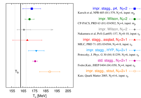
Fig. 1.: Summary of lattice results on the transition temperature $T_{c}$ taken from Refs. [19, 20, 21, 22, 24, 25] as well as unpublished result from S. Katz presented on Quark Matter 2005. The horizontal line and the band is the chemical freezout temperature at the highest RHIC energy [26].

3 Charmonia correlators and spectral functions

In lattice QCD we calculate correlators of point meson operators of the form

$$J_{H}(t,x)=\bar{q}(t,x)\Gamma_{H}q(t,x),$$ (1)

where $\Gamma_{H}=1,\gamma_{5},\gamma_{\mu},\gamma_{5}\gamma_{\mu},\gamma_{\mu}\gamma_{\nu}$ and fixes the quantum number of the channel to scalar, pseudo-scalar, vector, axial-vector and tensor channels correspondingly. The relation of these quantum number channels to different meson states is given in Tab. 1. Most dynamic properties of a finite temperature system are incorporated in the spectral function. The spectral function $\sigma(p_{0},\vec{p},T)$ for a given mesonic channel $H$ in a system at temperature $T$ can be defined through the Fourier transform of the real time two-point functions $D^{>}(x_{0},\vec{x},T)$ and $D^{<}(x_{0},\vec{x},T)$ or, equivalently, as the imaginary part of the Fourier transformed retarded correlation function [28]. The Euclidean time correlator calculated on the lattice

$$G_{H}(\tau,\vec{p},T)=\int d^{3}xe^{i\vec{p}\cdot\vec{x}}\langle T_{\tau}J_{H}(\tau,\vec{x})J_{H}(0,\vec{0})\rangle$$ (2)

is an analytic continuation of the real time correlator $G_{H}(\tau,\vec{p},T)=D^{>}(-i\tau,\vec{p},T)$. Using this fact and the Kubo-Martin-Schwinger (KMS) condition [28] for the correlators $D^{>}_{H}(x_{0},\vec{x},T)=D^{<}(x_{0}+i/T,\vec{x},T)$, one can relate the Euclidean propagator $G_{H}(\tau,\vec{p},T)$ to the spectral function through the integral representation

$$G(\tau,\vec{p},T) = \int_{0}^{\infty}d\omega\sigma(\omega,\vec{p},T)K(\omega,\tau,T)$$

$$K(\omega,\tau,T) = \frac{\cosh(\omega(\tau-1/2T))}{\sinh(\omega/2T)}.$$ (3)

$\Gamma$	${}^{2S+1}L_{J}$	$J^{PC}$	$u\overline{u}$
$\gamma_{5}$	${}^{1}S_{0}$	$0^{-+}$	$\pi$
$\gamma_{s}$	${}^{3}S_{1}$	$1^{--}$	$\rho$
$\gamma_{s}\gamma_{s^{\prime}}$	${}^{1}P_{1}$	$1^{+-}$	$b_{1}$
$1$	${}^{3}P_{0}$	$0^{++}$	$a_{0}$
$\gamma_{5}\gamma_{s}$	${}^{3}P_{1}$	$1^{++}$	$a_{1}$

$c\overline{c}(n=1)$	$c\overline{c}(n=2)$
$\eta_{c}$	$\eta_{c}^{{}^{\prime}}$
$J/\psi$	$\psi^{\prime}$
$h_{c}$
$\chi_{c0}$
$\chi_{c1}$

$b\overline{b}(n=1)$	$b\overline{b}(n=2)$
$\eta_{b}$	$\eta_{b}^{\prime}$
$\Upsilon(1S)$	$\Upsilon(2S)$
$h_{b}$
$\chi_{b0}(1P)$	$\chi_{b0}(2S)$
$\chi_{b1}(1P)$	$\chi_{b1}(2P)$

Table 1.: Meson states in different channels

To reconstruct the spectral function from the lattice correlator $G(\tau,T)$ this integral representation should be inverted. Since the number of data points is less than the number of degrees of freedom (which is ${\cal O}(100)$ for reasonable discretization of the integral ) spectral functions can be reconstructed only using the Maximum Entropy Method (MEM) [29]. In this method one looks for a spectral function which maximizes the conditional probability $P[\sigma|DH]$ of having the spectral function $\sigma$ given the data $D$ and some prior knowledge $H$ which for positive definite spectral function can be written as

$$P[\sigma|DH]=\exp(-\frac{1}{2}\chi^{2}+\alpha S),$$ (4)

where $S=\int d\omega[\sigma(\omega)-m(\omega)-\sigma(\omega)\ln(\sigma(\omega)/m(\omega))]$ is the Shannon - Janes entropy. The real function $m(\omega)$ is called the default model and parametrizes all additional prior knowledge about the spectral functions, such as the asymptotic behavior at high energy [29]. In order to have sufficient number of data points either very fine isotropic lattices [11, 12, 15] or anisotropic lattices [9, 10, 13, 14] have been used.

The spectral function for pseudo-scalar charmonium spectral functions calculated on anisotropic lattice [13] is shown in Fig. 2. The first peak in the spectral function corresponds to $\eta_{c}(1S)$ state. The position of the peak and the corresponding amplitude (i.e. the area under the peak) are in good agreement with the results of simple exponential fit. The second peak in the spectral function is most likely the combination of several excited states as its position and amplitude is higher than what one would expect for pure 2S state. The spectral function becomes sensitive to the effects of the finite lattice spacings for $\omega>5$GeV. In this $\omega$ region the spectral functions becomes also sensitive to the choice of the default model. Also shown in Fig. 2 is the spectral function in the scalar channel from Ref. [13]. The 1st peak corresponds to $\chi_{c0}(1P)$ state. The correlator is more noisy in the scalar channel than in the pseudo-scalar one. As the results the $\chi_{c0}(1P)$ peak is less pronounced and has larger statistical errors. The peak position and the area under the peak is consistent with the simple exponential fit. As in the pseudo-scalar case individual excited states are not resolved and the spectral function depends on the lattice spacing and default model for $\omega>5$GeV.

Fig. 2.: Charmonium spectral function in the pseudo-scalar channel (left) and the scalar channel (right) at different lattice spacings and zero temperature from Ref. [13].

Similar results have been found for the vector and axial-vector channels which correspond to $J/\psi$ and $\chi_{c1}$ states respectively.

We would like to know what happens to different charmonia states at temperatures above the deconfinement temperature $T_{c}$. With increasing temperature it becomes more and more difficult to reconstruct the spectral functions as both the number of available data points as well as the physical extent of the time direction (which is $1/T$) decreases. Therefore it is useful to study the temperature dependence of charmonia correlators first. From Eq. (3) it is clear that the temperature dependence of charmonia correlators come from two sources: the temperature dependence of the spectral function and the temperature dependence of the integration kernel $K(\tau,\omega,T)$. To separate out the trivial temperature dependence due to the integration kernel, following Ref. [12] for each temperature we calculate the so-called reconstructed correlator $G_{recon}(\tau,T)=\int_{0}^{\infty}d\omega\sigma(\omega,T=0)K(\tau,\omega,T).$ Now if we assume that there is no temperature dependence in the spectral function, then the ratio of the original and the reconstructed correlator should be close to one, $G(\tau,T)/G_{recon}(\tau,T)\sim 1$. This way we can identify large changes in the spectral function. This gives reliable information about the fate of charmonia states above deconfinement. In Fig. 3 we show this ratio for pseudo-scalar and scalar channels correspondingly calculated on anisotropic lattice [13].

Fig. 3.: The ratio $G(\tau,T)/G_{recon}(\tau,T)$ of charmonium for pseudoscalar channel at at $a_{t}^{-2}=14.11$GeV (left) and scalar channel at at $a_{t}^{-2}=8.18$GeV (right) at different temperatures [13].

From the figures one can see that the pseudo-scalar correlators shows only very small changes till $1.5T_{c}$ indicating that the $\eta_{c}$ state survives till this temperature with little modification of its properties. On the other hand the scalar correlator shows large changes already at $1.16T_{c}$ suggesting strong modification or dissolution of the $\chi_{c0}$ state at this temperature.

More detailed information on different charmonia states at finite temperature can be obtained by calculating spectral functions using MEM. The results of these calculations are show in Figs. 4. Because at high temperature the temporal extent and the number of data points where the correlators are calculated become smaller the spectral functions reconstructed using MEM are less reliable. To take into account possible systematic effects when studying the temperature modifications of the spectral functions we compare the finite temperature spectral functions against the zero temperature spectral functions obtained from the correlator using the same time interval and number of data points as available at finite temperature. We see that spectral function in the pseudo-scalar channel show no temperature dependence within the statistical errors. This is in accord with the analysis of the correlation functions. Also the spectral functions show very little dependence on the default model. Similar conclusion has been made in Ref. [11, 12] where correlators and spectral functions have been calculated on very fine isotropic lattices as well as in Ref. [10] where anisotropic lattice have been used. The pseudo-scalar spectral function was found to be temperature independent also in Ref. [9] where correlators of extended meson operators have been studied on anisotropic lattices. The study of the charmonium correlators with different spatial boundary conditions provides further evidence for survival of the $1S$ charmonia states well above the deconfinement transition temperature [30].

The scalar spectral function shows large changes at $1.16T_{c}$ which is consistent with correlator-based analysis. Also the default model dependence of the scalar correlator is large above the deconfinement transition (c.f. Fig. 3, right). This means that the $\chi_{c0}$ (${}^{3}P_{0}$) dissolves at this temperature. Similar results for the scalar spectral function have been reported in [11, 12]. The results for the axial correlators and spectral functions are similar to scalar ones [12] as expected.

Fig. 4.: Charmonia spectral function in the psuedoscalar channel at $a_{t}^{-2}=14.11$GeV (left) and the scalar channel (right) at $a_{t}^{-2}=8.18$GeV for zero and finite temperature [13]. For finite temperature scalar channel two different default models are shown.

The vector correlator, however, has temperature dependence different from that of the pseudo-scalar channel [31]. This is due to the fact that the vector current is conserved and there is a contribution to the spectral functions at very small energy $\omega\simeq 0$ corresponding to heavy quark transport [32, 33]. The transport peak in the spectral functions can be written as [32]

$$\sigma_{low}(\omega)=\chi_{s}(T)\frac{T}{M}\frac{1}{\pi}\frac{\omega\eta}{\omega^{2}+\eta^{2}},$$ (5)

where $\eta=T/M/D$ with $D$ being the heavy quark diffusion constant. Furthermore $\chi_{s}(T)$ is the charm or beauty susceptibility and $M$ is the heavy quark mass. To the first approximation the transport contribution to the spectral function gives rise to a positive constant contribution to the correlator $G_{low}(\tau)\simeq\chi_{s}(T)T^{2}/M$ [32], resulting in the enhancement of the finite temperature correlators relative to the zero temperature ones, in agreement with the lattice data presented in [31, 34]. Finite value of the diffusion constant $D$ will give rise to some curvature in $G_{low}(\tau)$. The smaller the value of $D$ is, the larger is the curvature in $G_{low}(\tau)$. Thus extracting $G_{low}(\tau)$ from lattice data and estimating its curvature can give an estimate for $D$. This, however, requires very precise lattice data which are not yet available [32].

4 Conclusions

In this contribution I discussed the status of finite temperature lattice QCD calculations. The transition in QCD appears to be a crossover and not a true phase transition. The value of the transition temperature, however, is not well know. Current lattice calculations give estimates between $167$ and $188$ MeV with large statistical and systematic errors. Recently charmonium correlators and spectral functions have been calculated in lattice QCD and show that $1S$ charmonia states survive above the transition temperatures till $1.6T_{c}$ while the $1P$ state dissolve at $T\simeq 1.1T_{c}$. Furthermore, the properties of the $1S$ charmonia states are not modified siginificantly above $T_{c}$. On the other hand potential model predict strong modification of charmonia properties and therefore are not consistent with the lattice data on the correlators presented above [33].

5 Acknowledgments

This work was supported by U.S. Department of Energy under Contract No. DE-AC02-98CH10886.

References

- [1] T. Matsui and H. Satz, Phys. Lett. B 178, 416 (1986)
- [2] F. Karsch, M. T. Mehr and H. Satz, Z. Phys. C 37, 617 (1988)
- [3] S. Digal, P. Petreczky and H. Satz, Phys. Lett. B 514, 57 (2001)
- [4] S. Digal, P. Petreczky and H. Satz, Phys. Rev. D 64, 094015 (2001)
- [5] E. V. Shuryak and I. Zahed, Phys. Rev. D 70, 054507 (2004)
- [6] C. Y. L. Wong, Phys. Rev. C 72, 034906 (2005)
- [7] W. M. Alberico, A. Beraudo, A. De Pace and A. Molinari, Phys. Rev. D 72, 114011 (2005)
- [8] P. Petreczky, Eur. Phys. J. C 43, 51 (2005)
- [9] T. Umeda, K. Nomura and H. Matsufuru, hep-lat/0211003
- [10] M. Asakawa and T. Hatsuda, Phys. Rev. Lett. 92, 012001 (2004)
- [11] S. Datta, F. Karsch, P. Petreczky and I. Wetzorke, hep-lat/0208012
- [12] S. Datta, F. Karsch, P. Petreczky and I. Wetzorke, Phys. Rev. D 69, 094507 (2004)
- [13] A. Jakovác, P. Petreczky, K. Petrov and A. Velytsky, hep-lat/0603005
- [14] K. Petrov, A. Jakovác, P. Petreczky, A. Velytsky, PoS (LAT2005), 153 (2005)
- [15] S. Datta, A. Jakovác, F. Karsch and P. Petreczky, hep-lat/0603002
- [16] M. Fukugita, M. Okawa, A. Ukawa, Phys. Rev. Lett. 63 , 1768 (1989)
- [17] E. Laermann and O. Philipsen, Ann. Rev. Nucl. Part. Sci. 53 , 163 (2003)
- [18] F. Karsch, E. Laermann, A. Peikert, Nucl. Phys. B 605, 579 (2001)
- [19] F. Karsch et al., Nucl. Phys. B (Proc. Suppl.) 129-130 , 614 (2004)
- [20] Z. Fodor and S. D. Katz, JHEP 0404, 050 (2004)
- [21] P. Petreczky, J. Phys. G 30 , S1259 (2004)
- [22] C. Bernard et al. [MILC Collaboration], Phys. Rev. D 71, 034504 (2005)
- [23] P. Petreczky and K. Petrov, Phys. Rev. D 70 , 054503 (2004)
- [24] A. Ali Khan et al. [CP-PACS Collaboration], Phys. Rev. D 63, 034502 (2002)
- [25] Y. Nakamura et al, PoS (LAT05), 157 (2005)
- [26] J. Adams et al (STAR Coll.), Nucl. Phys. A 757, 102 (2005)
- [27] P. Petreczky, Nucl. Phys. B ( Proc. Suppl. ) 140, 78 (2005)
- [28] M. Le Bellac, Thermal Field Theory , Cambridge University Press ,1996
- [29] M. Asakawa, T. Hatsuda and Y. Nakahara, Prog. Part. Nucl. Phys. 46, 459 (2001)
- [30] H. Iida, T. Doi, N. Ishii, H. Suganuma and K. Tsumura, hep-lat/0602008
- [31] P. Petreczky, K. Petrov, D. Teaney, A. Velytsky, hep-lat/0510021
- [32] P. Petreczky, D. Teaney, Phys. Rev. D 73 , 014508 (2006)
- [33] Á. Mócsy, P. Petreczky, Eur. Phys. J. C 43, 77 (2005), Phys. Rev. D 73, 074007 (2006)
- [34] S. Datta, F. Karsch, S. Wissel, P. Petreczky and I. Wetzorke, hep-lat/0409147