Simultaneous description of four positive and four negative parity bands

Abstract

The extended coherent state model is further extended in order to describe two dipole bands of different parities. The formalism provides a consistent description of eight rotational bands. A unified description for spherical, transitional and deformed nuclei is possible. Projecting out the angular momentum and parity from a sole state, the $K^{\pi}=1^{+}$ band acquires a magnetic character, while the electric properties prevail for the other band. Signatures for a static octupole deformation in some states of the dipole bands are pointed out. Some properties which distinguish between the dipole band states and states of the same parity but belonging to other bands are mentioned. Interesting features concerning the decay properties of the two bands are found. Numerical applications are made for ¹⁵⁸Gd, ¹⁷²Yb, ^228,232Th, ²²⁶Ra, ²³⁸U and ²³⁸Pu, and the results are compared with the available data.

I Introduction

The field of negative parity bands became very attractive when the first suggestions for a static octupole deformation were advanced by ChassmanCha , and Moler and Nix Mol . Since a nuclear shape with octupole deformation does not exhibit a space reflection symmetry and, on the other hand, a spontaneously broken symmetry leads to a new nuclear phase, one expects that the octupole deformed nuclei have specific properties. The main achievements of this field have been reviewed in Refs. Roho ; ButNaz ; Frau .

Identifying the nuclei which have static octupole deformation seems to be a difficult task. Indeed, because there is no measurable quantity for the octupole deformation, some indirect information about this variable should be found. Several properties are considered as signatures for octupole deformation: a) In some nuclei like ²¹⁸Ra, the state $1^{-}$, the head of the $K^{\pi}=0^{-}$ band, has a very low position, and this is an indication that the potential energy has a flat minimum, as a function of the octupole deformation. b) The parity alternating structure in ground and the lowest $0^{-}$ bands suggests that the two bands may be viewed as being projected from a sole deformed intrinsic state, exhibiting both quadrupole and octupole deformations. c) A nuclear surface with quadrupole and octupole deformations might have the centre of charge in a different position than the centre of mass, which results in having an electric dipole moment which may excite the state $1^{-}$ from the ground state, with a large probability. The list is not complete and thereby any new signature for this new nuclear phase deserves a special attention.

Few years ago we considered this subject within a phenomenological framework. Thus, in Refs. Rad8 ; Rad9 ; Rad10 ; Rad110 ; Rad13 we extended the coherent state model (CSM) Rad11 ; Rad12 to the negative parity bands. To the lowest positive parity bands, named ground ($g^{+}$), beta ($\beta^{+}$) and gamma ($\gamma^{+}$), one associates three negative bands, $g^{-}$, $\beta^{-}$, $\gamma^{-}$, respectively. The six bands are obtained by projecting out the angular momentum and the parity from three orthogonal functions which exhibit both quadrupole and octupole deformations. An effective boson Hamiltonian is considered in the space of angular momentum and parity projected states. The phenomenological boson model called Extended Coherent State Model (ECSM), has been successfully applied to a large number of nuclei, some of them being suspected to exhibit a static octupole deformation while some of them having vibrational octupole bands. Some signatures for a static octupole deformation in the excited bands have been pointed out.

In the present paper we extend even more the coherent state model by adding a new pair of parity partner bands. These are characterised by $K^{\pi}=1^{+}$ and $K^{\pi}=1^{-}$. Also two new terms are added to the model Hamiltonian without altering its effective character, whose strength are fixed by fitting some particular data for the new bands.

The new extension is presented according to the following plan. In Section II, a brief description of the CSM and ECSM is given. The scope consists in having a self-standing work and on the other hand in collecting the necessary definitions and notations. In section III, the ingredients of the new extension are presented in extenso, i.e. the properties of the states which enlarge the model boson space as well as the corrective terms of the model Hamiltonian and their matrix elements are analytically given. In Section IV, we discuss the numerical application for seven nuclei. Since for ¹⁷²Yb and ²²⁶Ra, some results were reported in two earlier publications, here we consider only the new results. A summary of the results and the final conclusions are presented in Section V.

II Brief review of the coherent state model and its extended version

II.1 The coherent state model (CSM)

In the beginning of eighties, one of the present authors (A. A. R) proposed, in collaboration, a phenomenological model to describe the main properties of the first three collective bands i.e., ground, beta and gamma bands Rad11 ; Rad12 . The model space was generated through a projection procedure from three orthogonal deformed states. The choice was made so that several criteria required by the existent data are fulfilled. The states are built up with quadrupole bosons and therefore we are dealing with those properties which are determined by the collective motion of the quadrupole degrees of freedom.

We suppose that the intrinsic ground state is described by a coherent state of Glauber type corresponding to the zeroth component of the quadrupole boson operator $b_{2\mu}$. The other two generating functions are the simplest polynomial excitations of the intrinsic ground state, chosen in such a way that the orthogonality condition is satisfied before and after projection. To each intrinsic state one associates an infinite rotational band. In two of these bands the spin sequence is $0^{+},2^{+},4^{+},6^{+},..$ etc., and therefore they correspond to the ground (the lowest one) and to the beta bands, respectively. The third one involves all angular momenta larger or equal to 2, and is describing, in the first order of approximation, the gamma band. The intrinsic states depend on a real parameter d which simulates the nuclear deformation. In the spherical limit, i.e. d goes to zero, the projected states are multi-phonon states of highest, second and third highest seniority, respectively. In the large deformation regime, conventionally called rotational limit (d equal to 3 means already a rotational limit), the model states behave like a Wigner function, which fully agrees the behaviour prescribed by the liquid drop model. The correspondence between the states in the spherical and rotational limits is achieved by a smooth variation of the deformation parameter. This correspondence agrees perfectly with the semi-empirical rule of ShelineShe and SakaiSaka , concerning the linkage of the ground, beta and gamma band states and the member of multi-phonon states from the vibrational limit. This property is very important when one wants to describe the gross features of the reduced probabilities for the intra and inter bands transitions.

In this restricted collective model space an effective boson Hamiltonian is constructed. A very simple Hamiltonian was found, which has only one off-diagonal matrix element, namely that one connecting the states from the ground and the gamma bands.

$$H_{CSM} = H_{2}^{\prime}+\lambda\hat{J}^{2}_{2},$$

$$H_{2}^{\prime} = A_{1}(22\hat{N}_{2}+5\Omega^{\dagger}_{\beta^{\prime}}\Omega_{\beta^{\prime}})+A_{2}\Omega^{\dagger}_{\beta}\Omega_{\beta},$$ (2.1)

where $\hat{N}_{2}$ denotes the quadrupole boson number operator

$$\hat{N}_{2}=\sum_{-2\leq m\leq 2}b_{2m}^{\dagger}b_{2m},$$ (2.2)

while $\Omega^{\dagger}_{\beta^{\prime}}$ and $\Omega^{\dagger}_{\beta}$ stand for the following second and third degree scalar polynomials:

$$\Omega^{\dagger}_{\beta^{\prime}} = (b^{\dagger}_{2}b^{\dagger}_{2})_{0}-\frac{d^{2}}{\sqrt{5}},$$

$$\Omega^{\dagger}_{\beta} = (b^{\dagger}_{2}b^{\dagger}_{2}b^{\dagger}_{2})_{0}+\frac{3d}{\sqrt{14}}(b^{\dagger}_{2}b^{\dagger}_{2})_{0}-\frac{d^{3}}{\sqrt{70}}.$$ (2.3)

The angular momentum carried by the quadrupole bosons, is denoted by $\hat{J}_{2}$. The boson states space is spanned by the projected states:

$$\varphi^{(i)}_{JM}=N^{(i)}_{J}P^{J}_{MK}\psi_{i},~{}~{}i=g,\beta,\gamma,$$ (2.4)

where the intrinsic states are:

$$\psi_{g}=e^{d(b^{{\dagger}}_{20}-b_{20})}|0\rangle,~{}~{}\psi_{\beta}=\Omega^{{\dagger}}_{\beta}\psi_{g},~{}~{}\psi_{\gamma}=\Omega^{{\dagger}}_{\gamma}\psi_{g}.$$ (2.5)

The excitation operator $\Omega^{{\dagger}}_{\beta}$ is given by Eq.(2.3), while the operator $\Omega^{{\dagger}}_{\gamma}$, which excites the gamma band states, is:

$$\Omega^{{\dagger}}_{\gamma}=(b^{{\dagger}}_{2}b^{{\dagger}}_{2})_{22}+d\sqrt{\frac{2}{7}}b^{{\dagger}}_{22}.$$ (2.6)

The angular momentum projection operator is defined by:

$$P^{J}_{MK}=\frac{2J+1}{8\pi^{2}}\int D^{J^{*}}_{MK}(\Omega)\hat{R}(\Omega)d\Omega,$$ (2.7)

where the standard notations for the Wigner function and the rotation operator corresponding to the Eulerian angles $\Omega$, have been used.

The eigenvalues of the effective Hamiltonian in the restricted space of projected states have been analytically studied in both spherical and rotational limit. Compact formulae for transition probabilities in the two extreme limits have been also derived. This model has been successfully applied for a large number of nuclei from transitional and well deformed regions. It is worth to mention that by varying the deformation parameter and the parameters defining the effective Hamiltonian one can realistically describe nuclei satisfying various symmetries like, SU(5) (Sm region)RadSand , O(6) (Pt region)Rad11 ; Rad12 , SU3 (Th region)RaSab , triaxial rotor (Ba, Xe isotopes)UliRad . This model has been extended by including the coupling to the individual degrees of freedom RadCels . In this way the spectroscopic properties in the region of back-bending were quantitatively described.

The extension of the CSM formalism, which will be presented here, considers a composite system of quadrupole and octupole bosons.

II.2 The extended coherent state model (ECSM)

The CSM formalism was generalised by assuming that the intrinsic ground state exhibits not only a quadrupole deformation but also an octupole one. Since the other bands, beta and gamma, are excited from the ground state, they also have this property. The octupole deformation is described by means of an axially symmetric coherent state for the octupole bosons $b^{{\dagger}}_{30}$. Thus, the intrinsic states for ground, beta and gamma bands are:

$$\Psi_{g}=e^{f(b^{{\dagger}}_{30}-b_{30})}e^{d(b^{{\dagger}}_{20}-b_{20})}|0\rangle_{(3)}|0\rangle_{(2)},~{}\Psi_{\beta}=\Omega^{{\dagger}}_{\beta}\Psi_{g},~{}\Psi_{\gamma}=\Omega^{{\dagger}}_{\gamma}\Psi_{g}.$$ (2.8)

The notation $|0\rangle_{(k)}$ stands for the vacuum state of the $2^{k}$-pole boson operators. Note that any of these states is a mixture of positive and negative parity states. Therefore they don’t have good reflection symmetry. Due to this feature the new extension of the CSM formalism has to project out not only the angular momentum but also the parity. The parity projection affects only the factor function depending on octupole bosons. Useful simplifications are achieved when this factor function is separately treated. The parity projected states are defined by:

$$\Psi^{(k)}_{oc}=P^{(k)}e^{f(b^{{\dagger}}_{30}-b_{30})}|0\rangle_{(3)},k=\pm,$$ (2.9)

where $P^{(k)}$ denotes the parity projection operator which is defined by its property that acting on a state consisting of a series of boson operators acting on the octupole vacuum, it selects only components with even powers in bosons if $k=+$ and odd components for $k=-$. From the parity projected states one projects out, further, the components with good angular momentum:

$$\Psi^{(k)}_{oc;J_{3}M_{3}}=N^{(k)}_{oc;J_{3}}P^{J}_{M_{3}0}\Psi^{(k)}_{oc}.$$ (2.10)

The factor $N^{(k)}_{oc;J_{3}}$ assures that the projected state has the norm equal to unity. Its expression is given in Appendix A.

Then, the intrinsic states of good parity are defined by:

$$\Psi^{(k)}_{i}=\Psi^{(k)}_{oc}\Psi_{i},~{}i=g,\beta,\gamma,~{}k=\pm.$$ (2.11)

The member states of ground beta and gamma bands are projected from the corresponding intrinsic states:

$$\varphi_{JM}^{(i,k)} = {\cal N}_{J}^{(i,k)}P_{MK_{i}}^{J}\Psi_{i}^{(k)},~{}~{}K_{i}=2\delta_{i,\gamma},~{}~{}k=\pm;i=g,\beta,\gamma,$$ (2.12)

$$J=(\delta_{i,g}+\delta_{i,\beta})(even\delta_{k,+}+odd\delta_{k,-})+\delta_{i,\gamma}(J\geq 2).$$

It can be shown that these projected states can be expressed by means of the octupole factor projected states and the projected states characterising the CSM formalism.

$$\varphi^{(i,k)}_{JM}={\cal N}^{(i,k)}_{J}\sum_{J_{2},J_{3}}\left(N^{(k)}_{oc;J_{3}}N^{(i)}_{J_{2}}\right)^{-1}C^{J_{3}~{}J_{2}~{}J}_{0~{}~{}K_{i}~{}~{}K_{i}}\left[\Psi^{(k)}_{oc;J_{3}}\varphi^{(i)}_{J_{2}}\right]_{JM},K_{i}=2\delta_{i,\gamma},~{}~{}k=\pm;i=g,\beta,\gamma,$$ (2.13)

The normalisation factor has the expression:

$$({\cal N}_{J}^{(i,k)})^{-2}=\sum_{J_{2},J_{3}}(N_{oc;J_{3}}^{(k)}N_{J_{2}}^{(i)})^{-2}(C_{0\hskip 7.11317ptK_{i}\hskip 5.69046ptK_{i}}^{J_{3}\hskip 2.84544ptJ_{2}\hskip 5.69046ptJ})^{2},~{}K_{i}=2\delta_{i,\gamma},~{}k=\pm;i=g,\beta,\gamma.$$ (2.14)

An effective boson Hamiltonian has been studied in the restricted collective space generated by the six sets of projected states. Note that from each of the three intrinsic states, one generates by projection two sets of states, one of positive and one of negative parity. When the octupole deformation goes to zero, the resulting states are just those characterising the CSM model. In this limit we know already the effective quadrupole boson Hamiltonian. When the quadrupole deformation is going to zero the system exhibits vibrations around an octupole deformed equilibrium shape. We consider for the octupole Hamiltonian an harmonic structure since the non-harmonic octupole terms can be simulated by the quadrupole anharmonicities. As for the coupling between quadrupole and octupole bosons, we suppose that this can be described by a product between the octupole boson number operator, $\hat{N}_{3}$, and the quadrupole boson anharmonic terms which are involved in the CSM Hamiltonian. Indeed, it has been proved that including octupole anharmonicities in the coupling terms these terms provide an angular moment dependence for the corresponding matrix elements similar to the one already generated by the terms involving only the operator $\hat{N}_{3}$ in the coupling with the quadrupole bosons. Also, the scalar product of the angular momenta carried by the quadrupole ($\vec{J}_{2}$) and octupole bosons ($\vec{J}_{3}$), respectively, and the total angular momentum squared ( $\vec{J}^{2}$), are included. Thus, the model Hamiltonian has the expression:

$$H = H^{\prime}_{2}+{\cal B}_{1}\hat{N}_{3}(22\hat{N}_{2}+5\Omega^{\dagger}_{\beta^{\prime}}\Omega_{\beta^{\prime}})+{\cal B}_{2}\hat{N}_{3}\Omega^{\dagger}_{\beta}\Omega_{\beta}$$ (2.15)

$$+{\cal B}_{3}\hat{N}_{3}+{\cal A}_{(J23)}\vec{J}_{2}\vec{J}_{3}+{\cal A}_{J}\vec{J}^{2}.$$

Detail arguments in favour of this choice are presented in our previous publication on this subject. This Hamiltonian was used in Refs.Rad8 ; Rad9 ; Rad10 to study the ground and $K^{\pi}=0^{-}$ bands. As was shown in the quoted papers, the coupling term $\vec{J}_{2}\vec{J}_{3}$ is necessary in order to explain the low position of the state $1^{-}$ in the even-even Ra isotopes. Indeed, this term is attractive in the state $1^{-}$ while for other angular momenta is repulsive.

Due to the specific structure of the CSM basis states the only non-vanishing off-diagonal matrix elements are those connecting the states of the ground and gamma and of the $0^{-}$ and $2^{-}$ bands. The energies of the six bands are defined as eigenvalues of the model Hamiltonian in the model space of the projected states. They depend on the structure coefficients ${\cal A}_{k}$,(k=1,2,J,(J23)) and ${\cal B}_{k}$ ,(k=1,3) defining the model Hamiltonian and the two deformation parameters, d and f. Therefore there are eight parameters which are to be determined, by fitting the data for excitation energies with the theoretical energies normalised to the ground state energy. For the considered isotopes, the structure coefficients obtained in this manner have a smooth behaviour when we change A or Z.

The connection between the present description and the rotational bands, as defined in the liquid drop model, was established in Refs. Rad12 .

Indeed, as shown in Ref.(Rad12 ) the projected states are linear superposition of states with definite K-quantum number. Moreover, in the asymptotic limit of the deformation parameter a single K prevails for each set of projected states, associated to the intrinsic unprojected states respectively. Assigning to each band that $K$ which labels the dominant component of the superposition quoted above, one may assert that the projected states given by Eq.(2.13) comprises two $K^{\pi}=0^{+}$, two $K^{\pi}=0^{-}$ one $K^{\pi}=2^{+}$ and one $K^{\pi}=2^{-}$ subsets. Note that the $K$ quantum number is equal to the eigenvalue of $J_{z}$, corresponding to the unprojected states $\Psi_{k}$ with $k=g,\beta,\gamma$. Thus, the symmetry breaking in the wave functions given by Eq.(2.8) is equivalent to choosing an auxiliary intrinsic frame of reference.

The bands associated to these quantum numbers are conventionally denoted by $g^{\pm}(K^{\pi}=0^{\pm})$, $\beta^{\pm}(K^{\pi}=0^{\pm})$ and $\gamma^{\pm}(K^{\pi}=2^{\pm})$.

III The dipole bands

Extending further the ECSM formalism, by adding some new bands with keeping the basic principles of CSM unaltered, is a difficult task. Indeed, first one has to find an intrinsic state which is orthogonal onto other three states defined so far. Moreover, the orthogonality property has to be preserved also after projecting the angular momentum and parity. Suppose that this step has been already overcome. The next step is then, to extend the model Hamiltonian by adding new terms which are mainly responsible for the description of the new states. The new Hamiltonian should be effective in the extended space of projected states, i.e. the off diagonal matrix elements are either equal to zero or very small comparing them with the diagonal ones.

In the present paper, we propose the following solution for the intrinsic state generating, through the angular momentum and parity projection, the member states of the dipole bands:

$$\Psi^{(1,\pm)}=\Omega^{{\dagger}}_{3}b^{{\dagger}}_{31}\Psi^{\mp}_{oc}\Psi_{g},\rm{where}\;\;\Omega^{{\dagger}}_{3}=\left(b^{{\dagger}}_{3}b^{{\dagger}}_{3}\right)_{0}+\frac{f^{2}}{\sqrt{7}}.$$ (3.1)

The states $\Psi^{(1,+)}$ and $\Psi^{(1,-)}$ are orthogonal since their scalar product involves the overlap of components with different number of bosons. Moreover, since $\Psi^{\pm}_{oc}$ are vacuum states for the operator $\Omega_{3}$, the intrinsic states for the dipole bands are orthogonal onto the intrinsic states associated with the bands $g^{\pm},\beta^{\pm},\gamma^{\pm}$. From these states one obtains two sets of angular momentum projected states:

$$\varphi^{(1,\pm)}_{JM}={\cal N}^{(1,\pm)}_{J}P^{J}_{M1}\Psi^{(1,\pm)},$$ (3.2)

with the projection operator defined by Eq. (2.7). The dipole projected state can be written in a tensorial form:

$$\varphi^{(1,\pm)}_{JM}={\cal N}^{(1,\pm)}_{J}\sum_{J_{2},J_{3}}C^{J_{3}\;J_{2}\;J}_{1\;\;\;0\;\;\;1}\left(N^{(\pm)}_{31;J}N^{(g)}_{J_{2}}\right)^{-1}\left[\varphi^{(\pm)}_{31,J_{3}}\varphi^{(g)}_{J_{2}}\right]_{JM},$$ (3.3)

where the octupole factor state is defined by:

$$\varphi^{(1,\pm)}_{31;JM}=N^{(\pm)}_{31;J}P^{J}_{M1}\Omega^{{\dagger}}_{3}b^{{\dagger}}_{31}\Psi^{\mp}_{oc}.$$ (3.4)

The norm factors ${\cal N}^{(1,\pm)}_{J},N^{(\pm)}_{31;J}$ are analytically given in Appendix A.

It is worth to mention an useful property of the projected state defined above. Taking into account the expression of $\vec{J}_{3}$ in terms of octupole bosons:

$$J^{(3)}_{\mu}=\sqrt{12}\left[b^{\dagger}_{3}b_{3}\right]_{1\mu},$$ (3.5)

one finds:

$$b^{\dagger}_{31}\Psi^{\mp}_{oc}=\frac{1}{{\cal A}}J^{(3)}_{1}\Psi^{\pm}_{oc},$$ (3.6)

where

$${\cal A}=-\sqrt{12}C^{3\;3\;1}_{1\;0\;1}f.$$ (3.7)

Commuting the angular momentum and the rotation operators, one arrives at the following expression for the octupole projected state:

$$\varphi^{(1,\pm)}_{31;JM}=N^{(\pm)}_{31;J}\frac{1}{{\cal A}}C^{J^{\prime}\;\;1\;\;J}_{0\;\;\;1\;\;\;1}\sum_{\mu,J^{\prime}}C^{J^{\prime}\;\;1\;\;J}_{M^{\prime}\;\;\mu\;\;M}J^{(3)}_{\mu}P^{J^{\prime}}_{M^{\prime}0}\Omega_{3}\Psi^{\pm}_{oc}.$$ (3.8)

Denoting the $K^{\pi}=0^{\pm}$ projected state by:

$$\varphi^{(\pm)}_{3;JM}=N^{(\pm)}_{3;J}P^{J}_{M0}\Omega^{{\dagger}}_{3}\Psi^{\pm}_{oc},$$ (3.9)

the equation (3.8) leads to:

$$\varphi^{(1,\pm)}_{31;JM}=N^{(\pm)}_{31;J}\frac{1}{{\cal A}}C^{J\;\;1\;\;J}_{0\;\;\;1\;\;\;1}\sqrt{J(J+1)}\left(N^{(\pm)}_{3;J}\right)^{-1}\varphi^{(\pm)}_{3;JM}.$$ (3.10)

Since the two projected states involved in the two sides of the above equation respectively, are both normalised to unity we have:

$$\varphi^{(1,\pm)}_{31;JM} = \varphi^{(\pm)}_{3;JM},$$

$$\left(N^{(\pm)}_{31;J}\right)^{-1} = \frac{1}{{\cal A}}C^{J\;\;1\;\;J}_{0\;\;\;1\;\;\;1}\sqrt{J(J+1)}\left(N^{(\pm)}_{3;J}\right)^{-1}.$$ (3.11)

This equation provides technical simplifications for calculating the matrix elements corresponding the dipole projected states.

Invoking the results obtained for the quantum number $K$, one can prove that the dipole projected states are $K^{\pi}=1^{\pm}$ states, respectively. For a given J the projected states of positive and negative parity are obviously orthogonal onto each other. Moreover, they are orthogonal on the states of similar angular momentum describing the member states of the six bands which were previously defined.

The dipole projected states are weakly coupled to the states of other bands by the ${\cal B}_{1}$ and ${\cal B}_{3}$ terms of H (2.15). Moreover, these terms give large contribution to the diagonal matrix elements involving the projected dipole states. Aiming at describing quantitatively the properties of the dipole states two terms are added to the model Hamiltonian.

$$\Delta H={\cal C}_{1}\Omega^{\dagger}_{3}\Omega_{3}+{\cal C}_{2}\Omega^{\dagger}_{3}\hat{N}_{2}\Omega_{3}.$$ (3.12)

The new terms affect only the diagonal matrix elements of the dipole states.Their strengths are fixed as follows: ${\cal C}_{2}$ is determined such that the corresponding contribution to the particular state energy, in the negative dipole band, cancels the one coming from the ${\cal B}_{1}$ term. ${\cal C}_{1}$ is fixed such that the measured excitation energy of the state $1^{-}$ is reproduced. With the new parameters determined in this way, the effect of the off diagonal matrix elements corresponding the ${\cal B}_{1}$ and ${\cal B}_{3}$ terms, on the energies in the two dipole bands amounts of a few keV. Due to this feature the energies of the two dipole bands are obtained as the corresponding average values of the model Hamiltonian, $H+\Delta H$.

IV Numerical results

IV.1 Parameter description

The formalism presented in the previous section has been numerically applied for seven nuclei: ¹⁵⁸Gd, ¹⁷²Yb, ²²⁶Ra, ²²⁸Th, ²³²Th, ²³⁸U, ²³⁸Pu. Since some results for ¹⁷²Yb and ²²⁶Ra were earlier reported Rad31 ; Rad32 , for these nuclei we mention only the features not presented there. The experimental data are taken from Refs. Sug ; Blo ; Lee (¹⁵⁸Gd), Gono ; Gai ; Wal ; Bal (¹⁷²Yb), Ell ; Wol ; Coc1 (²²⁶Ra), Har (²²⁸Th), Coc1 ; Sim ; Ale ; Shu ( ²³²Th ), Ale ; Shu ; Gai (²³⁸U), Shu ; Gai ; Led (²³⁸Pu). Moreover, three pairs of parity partner bands have been treated in Refs.Rad110 ; Rad12 ; Rad13 where, excepting the new strengths ${\cal C}_{1}$ and ${\cal C}_{2}$, all parameters have been fixed through the least square procedure.

These new parameters have been fixed as explained in the previous section. Since the dipole states energies are sensitive to changing ${\cal B}_{1}$ and ${\cal B}_{3}$, we change slightly the known values of these parameters in order to improve the agreement in the negative dipole band. However, changing the values of ${\cal B}_{1}$ and ${\cal B}_{3}$ affects some of calculated energies in the other six bands. Such corrections are washed out by a small change of one of the parameters ${\cal A}_{J},{\cal A}_{J23}$. We have checked for few cases that the results obtained in this way are similar to those provided by a least square procedure applied for all eight bands. The final results for the model parameters are listed in Table I.

	158Gd	172Yb	226Ra	228Th	232Th	238U	238Pu
d	3.0	3.68	3.0	3.1	3.25	3.9	3.9
f	0.3	0.3	0.8	0.3	0.3	0.6	0.3
${\cal A}_{1}$	21.49	26.94	20.29	17.72	14.26	20.64	18.84
${\cal A}_{2}$	-12.28	-17.68	-17.21	-12.67	-8.34	-9.59	-8.63
${\cal A}_{J}$	3.5	4.72	0.49	1.32	2.26	2.14	2.26
${\cal A}_{J23}$	15.0	4.70	7.17	8.38	6.00	5.00	5.00
${\cal B}_{1}$	-11.68	-24.29	-1.53	-2.79	-6.25	-11.97	-8.43
${\cal B}_{3}$	3414.62	8327.68	523.07	858.37	2047.04	4483.28	3254.09
${\cal C}_{1}$	-3096.52	-8853.24	-217.31	-603.58	-1879.04	-4663.88	-3265.85
${\cal C}_{2}$	285.93	594.45	38.18	68.16	152.87	295.64	206.29

Table 1: The deformation parameters $d$ and $f$ and the structure coefficients involved in the model Hamiltonian, obtained as described in the text, are listed for several isotopes. The deformations are dimensionless, while the remaining coefficients are given in units of keV.

IV.2 Dipole bands energies

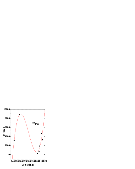
Figure 1: The structure coefficient ${\cal C}_{1}$, determined as explained in the text, is represented as function of $A-0.5*(N-Z)$ (black square). The obtained values are interpolated by a third order polynomial (full line curve).

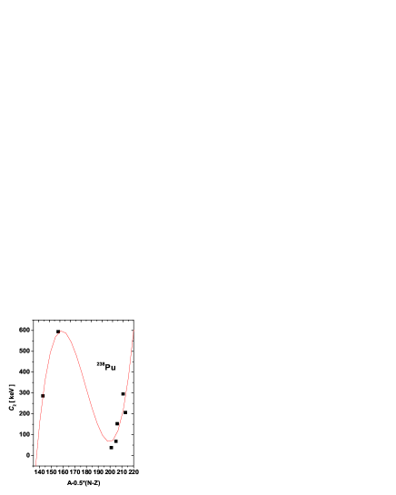
Figure 2: The structure coefficient ${\cal C}_{2}$, determined as explained in the text, is represented as function of $A-0.5*(N-Z)$ (black square). The obtained values are interpolated by a third order polynomial (full line curve).

As we have already suggested before, the calculated energies for $g^{\pm},\beta^{\pm},\gamma^{\pm}$ are practically the same as in Ref.Rad110 ; Rad12 ; Rad13 and therefore they are not given here. We stress on the fact that the volume of explained data with the mentioned parameters is quite large. For example, in the previously treated six bands of ²³²Th, about 55 excitation energies are known. Also, with the fixed deformation parameters, several experimental data concerning the transition reduced probabilities are realistically described. It is interesting to mention that these parameters have specific dependence on A and Z which means that applying the formalism to new cases, the strength parameters can be considered as fully determined from the previous analysis. As shown in Figs. 1 and 2, the new parameters ${\cal C}_{1}$ and ${\cal C}_{2}$ exhibit also a smooth dependence on the variable $A-0.5(N-Z)$. Adding the third isospin component to A we avoided the situation when for the isotopes of the same A one obtains different values of the considered parameters, which results in having a ill-defined function. The calculated energies for the dipole bands are collected in Tables II-V. Only the states with angular momentum not larger than 20 are listed. Note that except for ¹⁷²Yb, only few data are known for these bands. From the energy analysis, several common features can be seen. We note that in both $K^{\pi}=1^{-}$ and $K^{\pi}=1^{+}$ bands a doublet structure shows up. For us it is not clear whether this doublet structure is an indication of two bands of odd and even spins respectively. This suspicion is somehow confirmed in ²²⁸Th and ²²⁶Ra, where in the low part of the spectrum the doublet members have not a natural energy ordering.

	158Gd		172Yb		228Th		232Th
J+	Exp.	Th.	Exp.	Th.	Exp.	Th.	Exp.	Th.
1+	2.534	2.531	2.010	1.880		1.247	1.489	1.508
2+	2.539	2.563	2.047	1.897		1.250		1.519
3+	2.631	2.638		1.970		1.311	1.561	1.567
4+		2.698	2.073	1.984		1.301	1.573	1.578
5+		2.829		2.133		1.426		1.673
6+		2.927	2.156	2.139		1.409		1.687
7+		3.108		2.368		1.595		1.827
8+		3.256		2.370		1.587		1.851
9+		3.470		2.676		1.818		2.029
10+		3.681		2.683		1.832		2.073
11+		3.911		3.056		2.092		2.276
12+		4.189		3.078		2.139		2.347
13+		4.423		3.506		2.412		2.567
14+		4.771		3.552		2.497		2.669
15+		5.001		4.023		2.774		2.899
16+		5.417		4.101		2.899		3.033
17+		5.636		4.606		3.174		3.628
18+		6.118		4.719		3.338		3.435
19+		6.323		5.251		3.606		3.672
20+		6.870		5.403		3.808		3.871

Table 2: Experimental (left column) and theoretical (right column) excitation energies for the dipole band $K^{\pi}=1^{+}$ states are given in units of MeV for the isotopes ${}^{158}Gd,^{172}Yb,^{228}Th,^{232}Th$.

	226Ra		238U		238Pu
J+	Exp.	Th.	Exp.	Th.	Exp.	Th.
1+		1.363	1.354	1.367	1.310	1.343
2+		1.345		1.380		1.357
3+	1.422	1.420		1.425		1.401
4+		1.359		1.442		1.420
5+		1.526		1.531		1.506
6+		1.432		1.546		1.525
7+		1.684		1.684		1.656
8+	1.587	1.582		1.698		1.677
9+		1.896		1.882		1.851
10+		1.806		1.901		1.879
11+		2.158		2.126		2.092
12+		2.094		2.156		2.132
13+		2.465		2.413		2.376
14+		2.433		2.460		2.433
15+		2.812		2.743		2.702
16+		2.812		2.811		2.780
17+		3.193		3.113		3.067
18+		3.223		3.205		3.171
19+		3.602		3.521		3.471
20+		3.662		3.639		3.601

Table 3: The same as in Table II but for ${}^{226}Ra,^{238}U,^{238}Pu$.

	158Gd		172Yb		228Th		232Th
J-	Exp.	Th.	Exp.	Th.	Exp.	Th.	Exp.	Th.
1-	1.856	1.856	1.155	1.155	0.952	0.952	1.078	1.078
2-	1.895	1.912	1.198	1.207	0.968	0.989	1.100	1.110
3-	1.978	1.970	1.222	1.257		1.017		1.140
4-		2.091	1.331	1.375		1.104		1.213
5-		2.184	1.353	1.443		1.142		1.257
6-		2.366	1.541	1.636		1.281		1.372
7-		2.500	1.567	1.716		1.330		1.428
8-		2.727	1.828	1.986		1.512		1.582
9-		2.911	1.849	2.077		1.578		1.654
10-		3.165	2.193	2.421		1.791		1.839
11-		3.404	2.209	2.524		1.880		1.931
12-		3.672	2.630	2.935		2.113		2.140
13-		4.970	2.646	3.053		2.227		2.255
14-		4.237	3.134	3.523		2.470		2.479
15-		4.598		3.661		2.613		2.619
16-		4.857		4.182		2.860		2.854
17-		5.281		4.342		3.033		3.021
18-		5.526		4.906		3.277		3.261
19-		6.013		5.091		3.481		3.456
20-		6.240		5.692		3.719		3.699

Table 4: The same as in Table II, but for the $K^{\pi}=1^{-}$ band.

	226Ra		238U		238Pu
J-	Exp.	Th.	Exp.	Th.	Exp.	Th.
1-	1.080	1.049	0.967	0.967	0.963	0.863
2-	1.102	1.090	0.988	0.998	0.986	0.992
3-		1.108	1.035	1.033	1.019	1.025
4-		1.211	1.053	1.100	1.083	1.089
5-		1.227		1.153		1.138
6-		1.394		1.259		1.240
7-		1.409		1.326		1.302
8-		1.631		1.472		1.443
9-		1.647		1.553		1.516
10-		1.913		1.736		1.695
11-		1.933		1.831		1.781
12-		2.233		2.048		1.994
13-		2.258		2.157		2.093
14-		2.584		2.405		2.336
15-		2.619		2.529		2.450
16-		2.962		2.802		2.719
17-		3.012		2.942		2.851
18-		3.365		3.237		3.140
19-		3.434		3.392		3.291
20-		3.790		3.707		3.597

Table 5: The same as in Table III but for the $K^{\pi}=1^{-}$ band.

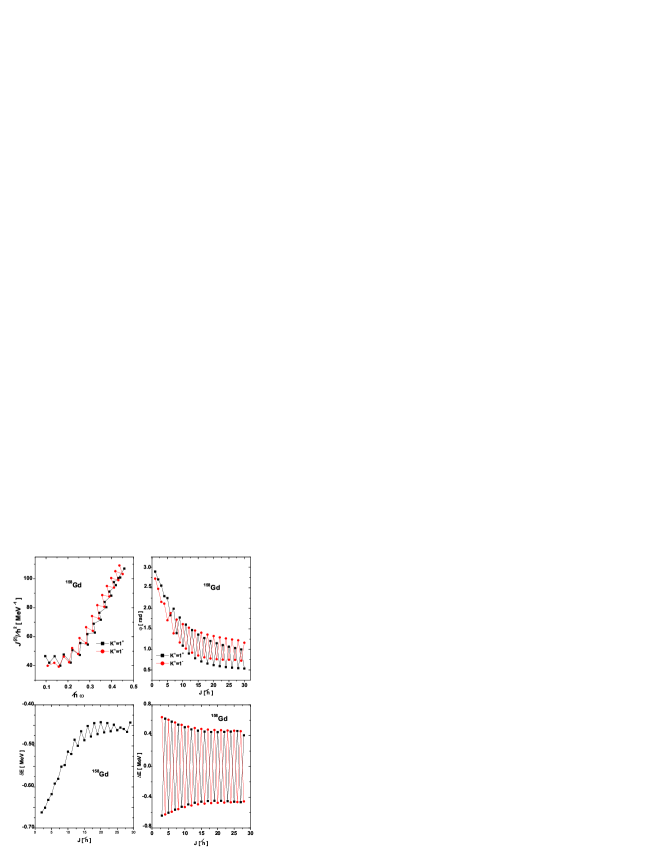
Figure 3: Upper left panel: The dynamic moment of inertia is plotted as function of angular frequency. Upper right panel: The angle between the angular momenta $\vec{J}_{2}$ and $\vec{J}_{3}$ is represented as function of angular momentum. Low-left panel: the first order energy displacement function is plotted vs. angular momentum. Low-right panel: the second order energy displacement is plotted as function of angular momentum. All theoretical results correspond to ¹⁵⁸Gd.

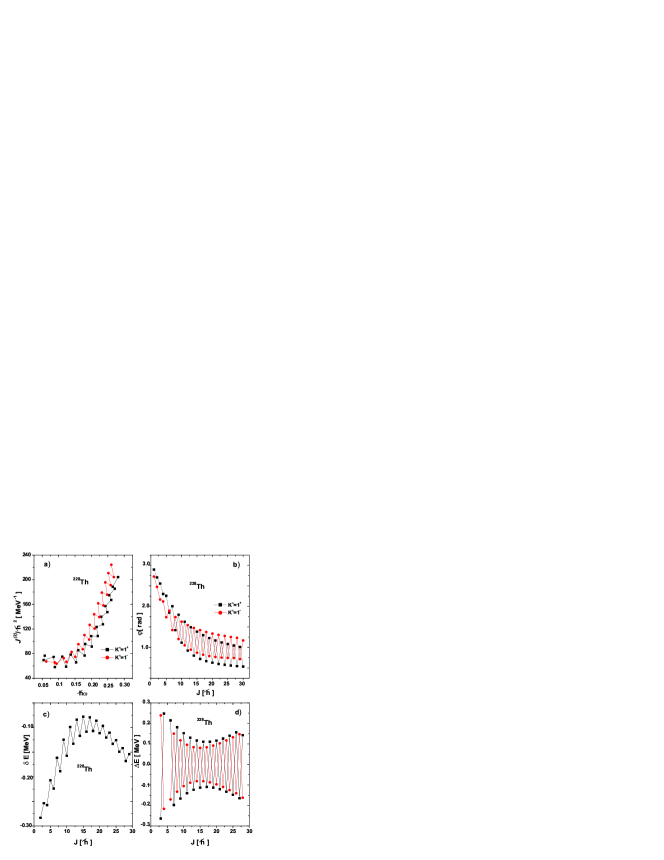
Figure 4: The same as in Fig. 3 but for ²²⁸Th.

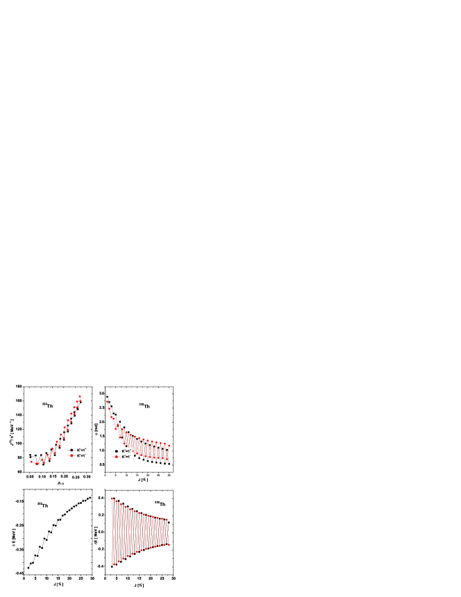
Figure 5: The same as in Fig. 3 but for ²³²Th.

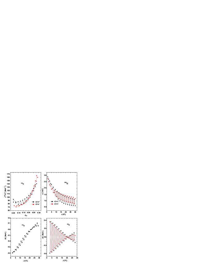
Figure 6: The same as in Fig. 3 but for ²³⁸U.

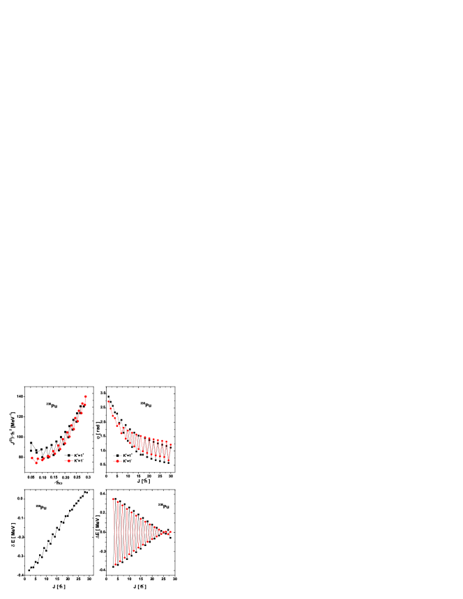
Figure 7: The same as in Fig. 3 but for ²³⁸Pu.

The excitation energies were further used to represent, in Figs. 3-7, the dynamic moment of inertia as function of angular frequency defined as:

$$\hbar\omega_{I} = \frac{dE}{dI}\approx\frac{1}{2}(E_{I}-E_{I-2}),$$

$$\frac{{\cal J}^{(2)}}{\hbar^{2}} = \left(\frac{d\hbar\omega}{dI}\right)^{-1}\approx\frac{2}{\hbar(\omega_{I}-\omega_{I-2})}.$$ (4.1)

The common feature of the moments of inertia is the zigzag structure in both, the negative and positive parity bands. For the $1^{+}$ band, the moments of inertia of odd and even spins are lying on smooth curves, respectively. The curve for the odd spins lies above that of even spins. The same is true also for the negative dipole band with the difference that the curve corresponding to the even angular momenta is higher than that for odd values of angular momentum. Due to the relative position of the four curves comprising the moments of inertia of even and odd spin states of positive and negative parity respectively, for some nuclei (¹⁷²Yb, ²²⁶Ra, ²³⁸U and ²³⁸Pu) it turns out that for some ranges of angular momenta the (odd,positive);(even, negative) and (even,positive); (odd,negative) states have moments of inertia lying on similar curves, respectively. This interleaved structure might be a signature for an octupole deformation in these states. In order get a confirmation for such an expectation we plotted in the low panels of the above quoted figures the first and second order energy displacement functions defined as:

$$\delta E(J^{-}) = E(J^{-})-\frac{(J+1)E((J-1)^{+})+JE((J+1)^{+})}{2J+1},$$

$$\Delta E_{1,\gamma}(J) = \frac{1}{16}\left[6E_{1,\gamma}(J)-4E_{1,\gamma}(J)-4E_{1,\gamma}(J)+E_{1,\gamma}(J)+E_{1,\gamma}(J)\right],$$

$$E_{1,\gamma}(J) = E(J+1)-E(J).$$ (4.2)

If the parity partner bands have similar J(J+1) pattern in a certain range of angular momentum, then the function $\delta E$ is vanishing for I belonging to the mentioned range. The reverse statement, if valid, asserts that for the angular momenta where the first order displacement function vanishes, the partner bands have identical moments of inertia which further infer that the two bands can be viewed as being associated to a sole intrinsic state. However, the J dependence of the excitation energies for the considered nuclei deviates from the J(J+1) law. If the energies can be described by a second order polynomial in $J(J+1)$ and moreover, the partner bands are characterised by the same strength for the $\left[J(J+1)\right]^{2}$ term, the second order energy displacement function is vanishing. Reversely, if $\Delta E_{1,\gamma}$ is vanishing, this is a sign that the two partner bands have similar $\left[J(J+1)\right]^{2}$ pattern. Concerning the second order energy displacement function, one should mention that there are two distinct functions of angular momentum differing by the set of states involved. In one function the lowest state is $1^{+}$ (the black squares) while for the other function the state $1^{-}$ is the lowest in energy. The parity assignment for the states involved in $\Delta E$ is conventionally taken as follows. The states whose angular momenta differ by two units have the same parity while those which differ by unity are of different parities. Inspecting Figs. 6, 7 from the present paper and 3 of Refs.(Rad31 ; Rad32 ) we remark that for ¹⁷²Yb, ²³⁸U, and ²³⁸Pu the second order energy displacements vanish for 2-3 consecutive values of angular momenta, while for ²²⁶Ra this is zero or very close to zero for $I\geq 11$.

In the right upper corner of Figs. 3-7, we plotted the angle between the angular momenta carried by the quadrupole and octupole bosons , respectively in the dipole states of positive as well as of negative parity. Such angle is defined as:

$$\cos\varphi=\frac{\langle\varphi^{(k)}_{JM}|\vec{J}_{2}\cdot\vec{J}_{3}|\varphi^{(k)}_{JM}\rangle}{\sqrt{\langle\varphi^{(k)}_{JM}|\hat{J}^{2}_{2}|\varphi^{(k)}_{JM}\rangle\langle\varphi^{(k)}_{JM}|\hat{J}^{2}_{3}|\varphi^{(k)}_{JM}\rangle}},\;\;k=1,+;1,-.$$ (4.3)

Note that this angle is a decreasing function of angular momentum and that the angles for odd and even spin states of positive parity, respectively are lying on smooth curves. The same is true for the angles characterising the negative parity band. Moreover, for $I\leq 7$ the curves for odd spin states of positive parity and for even spin states of negative parity are very close to each other. The same is valid for the curves of even spin and positive parity and odd spin states of negative parity. Similarly, one could calculate the angle between the two angular momenta in the other parity partner bands. Here we give the results for the bands $0^{+}$ and $0^{-}$ in Figs. 8 and 9. For these bands we didn’t consider the admixture with the gamma band states of similar angular momenta, since the numerical results for the isotopes considered, the mixing amplitudes are small. For a better presentation we omitted the state $0^{+}$ where the angle is equal to $\pi$. The angles for the two bands exhibit minima which are achieved for different values of angular momenta. However, for ²²⁶Ra and ²³⁸U the two minima are almost equal to each other and are reached for close values of angular momenta. After reaching the minima the angles increase and approach the limit value of $\frac{\pi}{2}$ in both bands. In the remaining cases this limit is met first by the band $0^{-}$ and much later in the ground band. Let us comment on the states where the angular momenta determined by the quadrupole and octupole bosons respectively, are perpendicular on each other respectively. The system under such a state constitute a precursor of a chiral symmetry Frau1 . Indeed, we could imagine a system of nucleons moving around a phenomenological core described by the quadrupole-octupole boson Hamiltonian considered here. Suppose that the coupling of the particle and core subsystems is such that the angular momentum carried by particles, say $\vec{j}$, is perpendicular to the plane $(\vec{J}_{2},\vec{J}_{3})$. If the system energy corresponding to the situation when the set $(\vec{j},\vec{J}_{2},\vec{J}_{3})$ form a right triad is degenerate with the energy corresponding to the situation when the three vectors define a left triad, one says that the system has a chiral symmetry. Of course, such a situation is an ideal picture and in practice one expects that the two energies are only approximatively degenerate. The symmetry breaking is expected to yield some properties which are specific for the new nuclear phase.

IV.3 Electromagnetic transition probabilities

The E1 and M1 transitions are determined by the following transition operators:

$$E_{1\mu} = T^{(h)}_{1\mu}+T^{(anh)}_{1\mu},$$

$$T^{(h)}_{1\mu} = q_{h}\sum_{\mu_{2},\mu_{3}}C^{3\;\;2\;\;1}_{\mu_{3}\;\mu_{2}\;\mu}\left(b^{\dagger}_{3\mu_{3}}+(-)^{\mu_{3}}b_{3,-\mu_{3}}\right)\left(b^{\dagger}_{2\mu_{2}}+(-)^{\mu_{2}}b_{2,-\mu_{2}}\right),$$

$$T^{anh}_{1\mu} = \left[b^{{\dagger}}_{3}\left(\hat{J}_{3}\hat{J}_{2}\right)\right]_{1\mu}+\left[\left(\hat{J}_{2}\hat{J}_{3}\right)b_{3}\right]_{1\mu},$$

$$M_{1\mu} = g_{2}\left(\hat{J}_{2}\right)_{\mu}+g_{3}\left(\hat{J}_{3}\right)_{\mu}$$ (4.4)

$$+ g^{\prime}_{2}\left[\left(\hat{J}_{2}\left(b^{{\dagger}}_{3}b^{{\dagger}}_{3}\right)_{2}\right)_{1\mu}+\left(\left(b_{3}b_{3}\right)_{2}\hat{J}_{2}\right)_{1\mu}\right]$$

$$+ g^{\prime}_{3}\left[\left(\hat{J}_{3}\left(b^{{\dagger}}_{2}b^{{\dagger}}_{2}\right)_{2}\right)_{1\mu}+\left(\left(b_{2}b_{2}\right)_{2}\hat{J}_{3}\right)_{1\mu}\right].$$

The reduced matrix elements ^∗) of interest for these operators are given analytically in Appendix C. Let us first discuss the magnetic properties of the dipole bands. Firstly, we calculated the gyromagnetic factors for the states of the two bands by considering only the lowest order boson terms in the expression of the $M1$ transition operator. In Ref.Rad200 we derived an expression for the M1 transition operator by quantising its classical expression. The important result was that the gyromagnetic factors $g_{2}$ and $g_{3}$ were expressed in terms of the Hamiltonian structure coefficients.The values obtained for ²³⁸U are:

$$g_{2}=0.371\mu_{N},\;\;g_{3}=2.266\mu_{N}.$$ (4.5)

These values have been adopted for all nuclei considered here. The results are presented in Tables VI and VII. We remark that the gyromagnetic factor of the state $2^{-}$ is very close to the phenomenologically adopted value for nuclei in the ground state, i.e. $Z/A$. This value is met in the positive parity band for the state $13^{+}$. The gyromagnetic factor of even spin states of positive parity is constantly much larger than those of negative parity. By contrary, the odd spin states of positive and negative parity have close gyromagnetic factors. For $J\leq 5$ the odd spin states of positive parity have gyromagnetic factors which are slightly larger than those characterising the odd spin states of negative parity. Starting with $J=7$, the ordering of gyromagnetic factors of odd spin states in the two bands is changed.

	158Gd		172Yb		228Th		232Th
J	$K^{\pi}=1^{+}$	$K^{\pi}=1^{-}$	$K^{\pi}=1^{+}$	$K^{\pi}=1^{-}$	$K^{\pi}=1^{+}$	$K^{\pi}=1^{-}$	$K^{\pi}=1^{+}$	$K^{\pi}=1^{-}$
1	0.645	0.865	0.645	0.789	0.645	0.851	0.645	0.832
2	1.081	0.403	0.859	0.379	1.042	0.399	0.989	0.392
3	0.503	0.548	0.424	0.452	0.489	0.530	0.469	0.506
4	0.939	0.316	0.760	0.286	0.910	0.310	0.869	0.302
5	0.476	0.486	0.395	0.405	0.461	0.472	0.441	0.452
6	0.821	0.293	0.697	0.263	0.803	0.386	0.776	0.280
7	0.457	0.448	0.381	0.383	0.444	0.437	0.425	0.422
8	0.723	0.281	0.642	0.254	0.712	0.276	0.695	0.269
9	0.439	0.417	0.372	0.366	0.428	0.409	0.412	0.398
10	0.645	0.273	0.592	0.249	0.638	0.269	0.627	0.263
11	0.422	0.391	0.363	0.352	0.412	0.386	0.398	0.377
12	0.584	0.267	0.548	0.245	0.579	0.263	0.573	0.258
13	0.406	0.370	0.355	0.340	0.398	0.366	0.386	0.359
14	0.536	0.261	0.511	0.241	0.533	0.258	0.528	0.253
15	0.391	0.353	0.347	0.329	0.384	0.349	0.374	0.344
16	0.498	0.256	0.480	0.238	0.496	0.253	0.492	0.249
17	0.376	0.338	0.339	0.319	0.371	0.336	0.362	0.331
18	0.476	0.252	0.453	0.237	0.466	0.250	0.463	0.246
19	0.364	0.327	0.332	0.310	0.359	0.324	0.352	0.321
20	0.442	0.249	0.431	0.234	0.440	0.246	0.438	0.243

Table 6: Calculated gyromagnetic factors for the states belonging to the dipole $K^{\pi}=1^{+}$ (left column) and $K^{\pi}=1^{-}$ (right column) bands are given in units of nuclear magneton $\mu_{N}$, for ${}^{158}Gd,^{172}Yb,^{228}Th,^{232}Th$.

	226Ra		238U		238Pu
J	$K^{\pi}=1^{+}$	$K^{\pi}=1^{-}$	$K^{\pi}=1^{+}$	$K^{\pi}=1^{-}$	$K^{\pi}=1^{+}$	$K^{\pi}=1^{-}$
1	0.645	0.931	0.645	0.793	0.645	0.773
2	1.100	0.427	0.813	0.381	0.806	0.374
3	0.510	0.644	0.409	0.461	0.407	0.431
4	0.959	0.351	0.719	0.289	0.712	0.279
5	0.484	0.592	0.378	0.417	0.375	0.385
6	0.841	0.334	0.667	0.268	0.659	0.257
7	0.467	0.563	0.366	0.398	0.363	0.365
8	0.745	0.329	0.621	0.260	0.614	0.248
9	0.451	0.544	0.358	0.386	0.355	0.352
10	0.670	0.330	0.579	0.255	0.572	0.243
11	0.437	0.531	0.351	0.377	0.347	0.340
12	0.614	0.332	0.542	0.253	0.534	0.239
13	0.423	0.522	0.344	0.369	0.341	0.330
14	0.572	0.337	0.509	0.252	0.500	0.236
15	0.412	0.514	0.338	0.362	0.334	0.320
16	0.541	0.342	0.480	0.251	0.472	0.234
17	0.403	0.507	0.332	0.356	0.328	0.312
18	0.518	0.348	0.457	0.250	0.447	0.232
19	0.395	0.499	0.327	0.351	0.322	0.304
20	0.500	0.354	0.436	0.250	0.426	0.230

Table 7: Gyromagnetic factors for the states belonging to the dipole $K^{\pi}=1^{-}$ and $K^{\pi}=1^{+}$ bands.

The transition from the band $1^{+}$ to the ground band is caused by the anharmonic term of the transition operator, while the intraband transitions as well as the gyromagnetic factors have been calculated by using only the lowest order boson terms. The factors $g_{2}$ and $g_{3}$ have been taken as mentioned before. Therefore the branching ratios for the M1 transitions:

$$R^{10}_{++} = \left[\frac{\langle\varphi^{(1,+)}_{J}||M_{1}||\varphi^{(g,+)}_{J+1}\rangle}{\langle\varphi^{(1,+)}_{J}||M_{1}||\varphi^{(g,+)}_{J-1}\rangle}\right]^{2},$$

$$R^{11}_{++} = \left[\frac{\langle\varphi^{(1,+)}_{J}||M_{1}||\varphi^{(1,+)}_{J+1}\rangle}{\langle\varphi^{(1,+)}_{J}||M_{1}||\varphi^{(1,+)}_{J-1}\rangle}\right]^{2},$$

$$R^{11}_{--} = \left[\frac{\langle\varphi^{(1,-)}_{J}||M_{1}||\varphi^{(1,-)}_{J+1}\rangle}{\langle\varphi^{(1,-)}_{J}||M_{1}||\varphi^{(1,-)}_{J-1}\rangle}\right]^{2},$$ (4.6)

are free of any adjustable parameter. The calculated values for these ratios are given in Tables VIII and IX. The branching ratios to the ground band have a minimum for $7\leq J\leq 9$ and a maximum for $15\leq J\leq 15$. Exceptions are for ²³⁸U and ²³⁸Pu where the maximum values are reached for J=23. The dominant ratios are those for odd values of angular momentum. The same is true for the intraband transition for the band $1^{+}$.

By contrast, in the negative parity band the ratios corresponding to even angular momenta prevail. One notices that for ¹⁵⁸Gd, $R^{11}_{++}$ has a minimum value for $J=9$ while $R^{11}_{--}$ has a maximum for $J=8$. These extreme values change from one nucleus to another. The dominant intraband M1 transitions for the band $1^{+}$ are those from even spin states. Moreover, they increase with the angular momentum. For example, for ²³²Th the B(M1) value is 0.25$\mu_{n}^{2}$ for $J=2$ and 4.23$\mu_{N}^{2}$ for $J=30$. As for the band $1^{-}$ the dominant transitions are those from odd spin states. Indeed, for the isotope mentioned above the $B(M1)$ value increase from 0.45 for J=3 to 2.06 $\mu_{N}^{2}$ for $J=29$. Except for the first transitions ($2^{+}\to 1^{+}$) all others B(M1) values are larger than the ones associated to negative parity band. Due to these facts we say that the band $1^{+}$ has a dominant magnetic character. It is worth noting that while the collective magnetic states of scissors nature are determined by the angular vibration, in a scissors fashion, of the symmetry axis of the proton and neutron systems, that angle being quite small, here the angle between $\vec{J}_{2}$ and $\vec{J}_{3}$ (which might be assimilated with the angle between the axis of the maximal moments of inertia of the quadrupole and octupole systems, respectively) is large. In this respect we could call the magnetic states from the band $1^{+}$, shares like states.

	158Gd			172Yb			228Th			232Th
J	$1^{+}\to 0^{+}$	$1^{+}\to 1^{+}$	$1^{-}\to 1^{-}$	$1^{+}\to 0^{+}$	$1^{+}\to 1^{+}$	$1^{-}\to 1^{-}$	$1^{+}\to 0^{+}$	$1^{+}\to 1^{+}$	$1^{-}\to 1^{-}$	$1^{+}\to 0^{+}$	$1^{+}\to 1^{+}$	$1^{-}\to 1^{-}$
1	0.376			0.369			0.375			0.373
2			7.718			4.272			6.819			5.838
3	0.348	11.51		0.343	639.1		0.347	15.74		0.346	27.233
4			20.45			6.335			15.802			11.561
5	0.160	5.22		0.185	21.14		0.164	6.144		0.170	8.015
6			97.87			12.495			58.746			33.428
7	0.004	4.17		0.037	9.755		0.008	4.613		0.015	5.446
8			2326.			27.790			465.4			139.73
9	0.300	4.00		0.024	6.998		0.214	4.262		0.128	4.743
10			978.4			72.40			8901.			2025.
11	3.114	4.15		0.478	5.979		2.275	4.302		1.466	4.595
12			223.83			258.3			410.81			2105.
13	23.821	4.45		2.535	5.574		15.494	4.524		8.870	4.691
14			122.4			2548			172.680			353.6
15	549.2	4.84		11.065	5.455		189.61	4.848		66.498	4.916
16			87.86			6013.			110.845			173.6
17	506.6	5.28		60.088	5.493		1629.	5.238		1018.	5.220
18			71.37			680.7			84.690			116.47
19	108.7	5.77		1442.	5.627		146.60	5.670		281.311	5.576
20			61.92			294.14			70.747			90.154
21	60.94	6.28		624.06	5.825		70.577	6.133		94.363	5.968
22			55.79			181.68			62.177			75.443
23	40.07	6.81		138.12	6.066		48.986	6.617		57.697	6.386
24			51.42			132.16			56.352			66.146
25	37.76	7.36		73.40	6.345		39.639	7.118		43.756	6.825
26			48.06			105.31			52.066			59.725
27	33.71	7.90		49.53	6.598		34.548	7.618		36.520	7.259
28			45.68			91.05			49.189			55.694
29	31.07	8.41		37.29	6.768		31.257	8.082		31.951	7.649
30			5.171			6.167			5.338			5.568

Table 8: M1 branching ratios for the $K^{\pi}=1^{+}$ and $K^{\pi}=1^{-}$ bands for ¹⁵⁸Gd, ¹⁷²Yb, ²²⁸Th, ²³²Th.

	226Ra			238U			238Pu
J	$1^{+}\to 0^{+}$	$1^{+}\to 1^{+}$	$1^{-}\to 1^{-}$	$1^{+}\to 0^{+}$	$1^{+}\to 1^{+}$	$1^{-}\to 1^{-}$	$1^{+}\to 0^{+}$	$1^{+}\to 1^{+}$	$1^{-}\to 1^{-}$
1	0.376			0.368			0.368
2			15.218			4.408			3.821
3	0.350	10.097		0.344	2820.		0.343	1322.
4			222.04			6.857			5.144
5	0.165	4.760		0.192	37.780		0.190	42.575
6			152.144			14.929			9.061
7	0.007	3.819		0.050	13.244		0.048	14.215
8			29.201			41.279			17.435
9	0.220	3.640		0.006	8.489		0.007	8.989
10			14.793			190.47			36.714
11	2.315	3.717		0.263	6.769		0.283	7.135
12			10.067			1713.			88.845
13	15.399	3.901		1.412	6.005		1.508	6.323
14			7.908			416.9			282.24
15	171.476	4.127		5.457	5.652		5.888	5.959
16			6.768			113.8			1951
17	2646.	4.365		21.402	5.511		23.781	5.827
18			6.134			58.266			7584
19	171.74	4.596		123.16	5.491		149.878	5.832
20			5.786			37.904			1090.
21	79.553	4.815		1569.	5.547		1153.	5.923
22			5.612			27.941			411.09
23	54.482	5.017		443.44	5.651		355.806	6.073
24			5.552			22.205			237.69
25	43.842	5.207		131.47	5.797		118.581	6.277
26			5.566			18.540			165.70
27	38.210	5.383		68.75	5.896		64.481	6.430
28			5.636			16.357			132.42
29	34.744	5.543		44.709	5.909		42.722	6.475
30			0.469			1.318			6.480

Table 9: The same as in Table VIII but for ²²⁶Ra, ²³⁸U, ²³⁸Pu.

Comparing the values of $R^{11}_{++}$ with those describing the M1 branching ratios for the transitions relating the bands $1^{-}$ and $0^{-}$, one finds out that the former ones prevail. The dominant ratios for the transitions $1^{-}\to 0^{-}$ are those corresponding to even values for the angular momentum.

Now let us turn our attention to the electric transitions E1 and E3. In Tables X and XI we listed the calculated E1 branching ratios:

$$R^{10}_{+-} = \left[\frac{\langle\varphi^{(1,+)}_{J}||E_{1}||\varphi^{(g,-)}_{J+1}\rangle}{\langle\varphi^{(1,+)}_{J}||E_{1}||\varphi^{(g,-)}_{J-1}\rangle}\right]^{2},$$

$$R^{10}_{-+} = \left[\frac{\langle\varphi^{(1,-)}_{J}||E_{1}||\varphi^{(g,+)}_{J+1}\rangle}{\langle\varphi^{(1,-)}_{J}||E_{1}||\varphi^{(0,+)}_{J-1}\rangle}\right]^{2}.$$

Concerning the ratio $R^{10}_{-+}$, two situations have been considered, namely when the transition operator is harmonic and when the anharmonic term defined above has been included. In that case we need the ratio $q_{anh}/q_{h}$. This ratios are to be fixed so that a certain experimental data for the branching ratio is reproduced. Such experimental data are available for the cases of ¹⁷²Yb and ²²⁶Ra and the determined values for the ratio of anharmonic and harmonic weights of the transition operator are equal to -1.722 and -1.4 respectively. The first value has been adopted also for ¹⁵⁸Gd while the second value was assigned for the ratio characterising the remaining nuclei considered here.

	158Gd			172Yb			228Th			232Th
J	$1^{+}\to 0^{-}$	$1^{-}\to 0^{+}$	$1^{-}\to 0^{+}$	$1^{+}\to 0^{-}$	$1^{-}\to 0^{+}$	$1^{-}\to 0^{+}$	$1^{+}\to 0^{-}$	$1^{-}\to 0^{+}$	$1^{-}\to 0^{+}$	$1^{+}\to 0^{-}$	$1^{-}\to 0^{+}$	$1^{-}\to 0^{+}$
1		11.637	5.321		28.7	6.537		13.197	5.991		16.013	6.329
2	3.156			2.641			3.065			2.939
3		1.948	1.871		2.056	1.828		1.955	1.869		1.974	1.858
4	1.559			1.299			1.512			1.448
5		1.311	1.598		1.305	1.478		1.301	1.546		1.292	1.516
6	1.650			1.407			1.608			1.550
7		7.144	2.899		8.280	2.470		7.163	2.967		7.290	2.849
8	2.221			1.935			2.177			2.112
9		7.312	3.022		7.197	2.452		7.157	3.048		7.025	2.892
10	5.365			4.089			5.136			4.825
11		8.294	3.252		7.252	2.539		7.976	3.252		7.624	3.058
12	5.909			4.415			5.627			5.255
13		9.594	3.520		7.630	2.666		9.099	3.499		8.518	3.266
14	6.774			4.899			6.405			5.928
15		11.115	3.808		8.194	2.816		10.429	3.768		9.603	3.498
16	7.815			5.453			7.336			6.726
17		12.846	4.108		8.906	2.982		11.952	4.052		10.861	3.746
18	9.011			6.066			8.401			7.632
19		14.771	4.417		9.742	3.158		13.652	4.346		12.276	4.005
20	10.356			6.737			9.597			8.644
21		16.877	4.732		10.687	3.342		15.517	4.646		13.836	4.271
22	11.846			7.469			10.921			9.762
23		19.152	5.050		11.732	3.532		17.537	4.951		15.532	4.542
24	13.480			8.279			12.373			10.988
25		21.587	5.370		12.870	3.727		19.704	5.258		17.358	4.816
26	15.257			9.149			13.952			12.323
27		23.944	5.686		13.646	3.915		21.755	5.560		19.008	5.085
28	17.188			10.128			15.676			13.789
29		26.073	6.013		14.234	4.131		23.574	5.877		20.426	5.374
30

Table 10: Calculated E1 branching ratios for the $K^{\pi}=1^{+}$ and $K^{\pi}=1^{-}$ bands in the isotopes for ¹⁵⁸Gd, ¹⁷²Yb, ²²⁸Th, ²³²Th. Results given in the first and second columns are obtained with a harmonic structure for the transition operator while those listed in the third column correspond to an anharmonic structure given by Eq. (4.4) with $q_{anh}/q_{h}$ equal to $-1.722$ for ¹⁵⁸Gd and ¹⁷²Yb and $-1.4$ for $Th$ isotopes. These values were obtained by fitting the experimental value corresponding to the state $1^{-}$ in ¹⁷²Yb and ²²⁶Ra, respectively.

	226Ra			238U			238Pu
J	$1^{+}\to 0^{-}$	$1^{-}\to 0^{+}$	$1^{-}\to 0^{+}$	$1^{+}\to 0^{-}$	$1^{-}\to 0^{+}$	$1^{-}\to 0^{+}$	$1^{+}\to 0^{-}$	$1^{-}\to 0^{+}$	$1^{-}\to 0^{+}$
1		10.500	5.815		37.24	8.036		39.380	8.072
2	3.141			2.518			2.521
3		1.89	1.840		2.090	1.850		2.108	1.858
4	1.545			1.236			1.239
5		1.294	1.523		1.321	1.443		1.325	1.449
6	1.635			1.344			1.347
7		5.954	2.932		8.531	2.542		9.178	2.567
8	2.188			1.845			1.851
9		6.104	2.988		7.178	2.460		7.569	2.484
10	5.100			3.742			3.778
11		7.010	3.156		7.087	2.503		7.349	2.528
12	5.624			4.043			4.072
13		8.402	3.364		7.326	2.591		7.502	2.619
14	6.464			4.474			4.498
15		9.341	3.525		7.631	2.696		7.858	2.738
16	7.491			4.957			4.976
17		10.375	3.688		8.079	2.817		8.364	2.875
18	8.510			5.467			5.497
19		11.460	3.851		8.632	2.947		8.989	3.024
20	9.628			6.019			6.062
21		12.554	4.015		9.269	3.085		9.715	3.182
22	10.827			6.612			6.670
23		13.671	4.182		9.976	3.226		10.532	3.347
24	12.091			7.260			7.339
25		14.807	4.356		10.741	3.369		11.430	3.518
26	13.412			7.965			8.069
27		15.898	4.533		11.105	3.500		11.857	3.676
28	14.791			8.766			8.906
29		16.945	4.718		11.371	3.657		12.149	3.875
30

Table 11: Calculated E1 branching ratios for the $K^{\pi}=1^{+}$ and $K^{\pi}=1^{-}$ bands, in the isotopes ²²⁶Ra, ²³⁸U, ²³⁸Pu. Results given in the first and second columns are obtained with a harmonic structure for the transition operator, while those listed in the third column correspond to an anharmonic structure given by Eq. (4.4) with $q_{anh}/q_{h}=-1.4$. This value was obtained by fitting the experimental value corresponding to the state $1^{-}$ in ²²⁶Ra.

In Fig. 10, the calculated branching ratios for the transitions of the negative dipole band to the ground band are compared with the corresponding data for the case of ¹⁷²Yb. One notices a good agreement between the two sets of data. In Fig. 10 we also compare the calculated and experimental branching ratios for the band $0^{-}$. One sees that these ratios are slowly decreasing with J up to J=11 when a plateau is reached. By contrast, the branching for the dipole band is decreasing up to $J=5$, has a small maximum at $J=7$, a flat minimum at J=9 and then is increasing with J. Note that the dipole band has larger branchings than the band $0^{-}$. One notes that while the two experimental ratios for the band $0^{-}$ are quite well described by those predicted by the Alaga rule, i.e. 2.0 and 1.33 respectively large deviations for Alaga rule are seen for the branching ratios characterising the dipole band with $K^{\pi}=1^{-}$. For example for J=1 and 3 the experimental ratios are about 6.5 and 2 respectively while the predictions of the Alaga rule are 0.5 and 0.75. Our results and Alaga rule predictions are at variance not only in the region of low spin but also for high spin states. Indeed, for J larger than nine, the Alaga rule predictions are close to 0.9 while in our case, starting with J=9 where the attained value is equal to about 2.5, our calculated ratios are increasing with J.

In Fig. 11 we compare three sets of data, namely the theoretical and experimental branching ratios characterising the band $0^{-}$ and the branching ratio associated to the negative parity dipole band, in ²²⁶Ra. For a better representation, the dipole branching ratios have been divided by 5. Remarkable the fact that modulo the factor five, the calculated ratios for the two bands have similar behaviour as function of J. It is interesting to see how the matrix elements of the E1 transition operator depend on the angular momentum, for the bands with $K^{\pi}=0^{-}$ and $K^{\pi}=1^{-}$. Comparison of the two sets of matrix elements is made in Fig.12. Note that for $J=odd$, the matrix element is characterising the transition from the states $J^{-}$ to the state $(J-1)^{+}$ while for $J=even$, this links the states $J^{+}$ and $(J-1)^{-}$. For both situations an anharmonic structure for the transition operator has been considered. The parameters involved in the $T_{1\mu}$ operator have the values: $q_{anh}/q_{h}=-1.4$ and $q_{h}=10^{-2}fm$. We note that the matrix elements describing the transition of the dipole state $J^{-}$, multiplied by a factor of 5 stays quite close to the similar matrix elements characterising the band $0^{-}$.

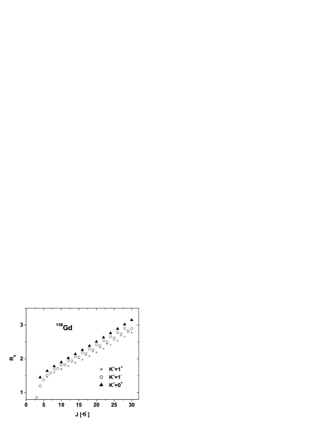
Figure 13: The B(E2) values for the intraband transitions for the $K^{\pi}=1^{+}$ and $K^{\pi}=1^{-}$ divided by the value corresponding to the transition $2^{\dagger}_{g}\to 0^{\dagger}_{g}$ are given as function of angular momentum. The ratio is denoted by $R_{q}$ according to Eq.(4.8). For comparison, the intraband B(E2) values characterising the ground band are also given.

In Fig. 13 we study the intraband E2 transitions in the two dipole bands. The calculated B(E2) values are divided by the B(E2) value corresponding to the transition $2^{\dagger}_{g}\to 0^{\dagger}_{g}$.

$$R_{q}=\frac{B(E2;J\to(J-2))}{B(E2;2^{+}_{g}\to 0^{+}_{g})}.$$ (4.8)

Results were obtained with a harmonic quadrupole transition operator and by neglecting the admixture of gamma band states in the structure of the ground band states. For comparison, we plotted also the reduced transition probability in the ground band, with a similar normalisation. The intraband quadrupole transitions have similar dependence on angular momentum in the two dipole bands. Moreover, the B(E2) values for the transitions $J^{-}\to(J-2)^{-}$ with J even lie close to the curve corresponding to the ground band.

The dipole bands may perform a E3 transition to the ground bands. To study the E3 properties of the dipole bands we have used an harmonic transition operator:

$$T_{3\mu}=q_{3}\left(b^{\dagger}_{3\mu}+(-)^{\mu}b_{3,-\mu}\right).$$ (4.9)

These transitions turns out to be weak. To have a flavour about the relative values of these transitions, comparing them to those from the band $0^{-}$, we normalise each transition to the B(E3) value associated for the transition $3^{-}_{g}\to 0^{+}_{g}$.

In Table XII we list the calculated values for the ratios:

$$T^{10}_{-+}(3;J) = \frac{B(E3,J^{-}\to(J+3)^{+}_{g})}{B(E3;3^{-}_{g}\to 0^{+}_{g})},$$

$$T^{10}_{+-}(3;J) = \frac{B(E3,J^{+}\to(J+3)^{-}_{g})}{B(E3;3^{-}_{g}\to 0^{+}_{g})}.$$ (4.10)

J	$T^{10}_{-+}(3;J)$	$T^{10}_{+-}(3;J)$
1	0.002
2		0.0
3	0.012
4		0.011
5	0.030
6		0.021
7	0.057
8		0.036
9	0.090
10		0.054
11	0.126
12		0.076
13	0.163
14		0.102
15	0.199
16		0.133
17	0.234
18		0.167
19	0.267
20		0.205
21	0.297
22		0.244
23	0.328
24		0.284
25	0.358
26		0.325
27	0.389

Table 12: The calculated values for the B(E3) values, normalized to the B(E3) value for the transition $3^{-}_{g}\to 0^{+}_{g}$, are listed for the transitions of the dipole band states of angular momentum J to the states of angular momentum (J+3) from the ground bands. The calculations were performed for ²²⁶Ra.

V Conclusions

In the previous sections we developed a formalism which appends the description of dipole bands to the extended coherent state model which results in obtaining a simultaneous and consistent model of eight rotational bands, four of positive and four of negative parity. Since for the seven nuclei considered, the results for three parity partner bands were already reported in some earlier publications here we focus on the description of the dipole bands. The present paper is the first which is devoted to the formalism description giving the analytical results describing the states and the matrix elements of the model Hamiltonian and transition operators.

The eight rotational bands are obtained by projecting out the angular momentum and parity, from four intrinsic states which are quadrupole and octupole deformed functions and moreover orthogonal onto each other. By construction the four states have the property that the eight sets of projected states are all orthogonal. The model states depend on two real parameters which simulate the quadrupole and octupole deformation, respectively. In the spherical limit i.e., both deformations tend to zero, specific multiphonon states of definite angular momentum, seniority and number of bosons respectively, are obtained. In the large deformation regime the projected states have a definite value for the $K$ quantum number. In the restricted space of projected states, an effective quadrupole-octupole boson Hamiltonian is considered. Indeed, for the model Hamiltonian the only nonvanishing matrix elements are those involving the states $(J^{\dagger}_{g},J^{\dagger}_{\gamma})$ with $J=even$ and $(J^{-}_{g},J^{-}_{\gamma})$ with $J=odd$. The structure coefficients defining the model Hamiltonian as well as the deformation parameters have been fixed by fitting through the least square procedure the energies in the bands $g^{\pm},\beta^{\pm},\gamma^{\pm}$ and the energy of the head state in the $K^{\pi}=1^{-}$ band. Also, one parameter (${\cal C}_{2}$ has been determined so that the contribution of the ${\cal B}_{3}$ term to a particular state ($2^{-}$) is canceled. This condition seems to be sufficient to decrease the off diagonal matrix elements involving the dipole band states to negligible values.

It is worth noting that dynamic moment of inertia of the odd and even angular momenta states are lying on separate smooth curves which could suggest that the two sets of states form distinct bands. This happens for both the positive and negative dipole bands. However, two pairs of these curves one for positive and one for negative subsets of states have an interleaved structure. These made us suspecting that an octupole static deformation shows up. In order to get a confirmation for this suspicion we calculated the first order and the second order energy displacement functions. Both functions vanish for similar angular momenta in ¹⁷²Yb, ²²⁶Ra, ²³⁸U and ²³⁸Pu. The only isotope where the vanishing persists in a relatively long range of angular momentum, is ²²⁸Ra. For other nuclei mentioned above the vanishing takes place in 1-3 states. In Ref.Rad31 we interpreted the vanishing of the displacement function for a very short interval of J in a way which conciliate between the band intersection and static octupole deformation. Indeed, for such states it may happen that they could be obtained by projection from an octupole deformed state which is different from the chosen model state for the dipole bands. Moreover, from this deformed state one could generate, through the angular momentum projection procedure, another two bands which are deformed all along and intersect the dipole bands considered here for the mentioned angular momentum. In this respect one could assert that bands intersection does not exclude the octupole deformation settlement.

Since the decay properties of the states depend on the corresponding boson structure, we calculated the angle between the angular momenta carried by the two kind of bosons. The result is that for high angular momentum states, this angle approaches the value $\pi/2$. This value is reached first in the negative and then in the positive band. Exception is for ²²⁶Ra and ²³⁸U where the angles in the two bands go simultaneously to the limit value $\pi/2$. We expect that for these systems, by adding a coupling set of particles one could reach a chirally symmetric picture.

For the sake of a complete description of the dipole states of positive and negative parity, by using the eigenstates of the model Hamiltonian, the intra and interband transitions of electric as well as of magnetic nature have been calculated. Comparison with the experimental data is made in terms of the branching ratios of the negative parity states. Also, these are compared with those characterizing the negative parity band with $K^{\pi}=0^{-}$. Also the gyromagnetic factors for the two bands were calculated. One notices a strong dependence on angular momentum for the gyromagnetic factors.

Comparing the intraband B(M1) values obtained for the two dipole bands, one concludes that the strength of magnetic transitions in the band $K^{\pi}=1^{+}$ is larger than that one associated with the band $K^{\pi}=1^{-}$. Due to this feature we say that the $K^{\pi}=1^{+}$ band has a magnetic nature. Concerning the $E1$ transition to the parity partner band of to the $g^{\pm}$ band, the strength order is changed. Therefore we say that the band $K^{\pi}=1^{-}$ has an electric nature. It is worth mentioning the role of parity projection in determining the magnetic or electric nature of the two bands.

Now let us say few words about the distinctive features of our formalism. The procedure is interesting not only because is able to describe a relatively large volume of data with a relatively small number of parameters, but also because it provides a consistent description of the rotational degrees of freedom. Indeed, all formalisms based on quadrupole and octupole boson interaction overestimate the contribution of the rotational degrees of freedom. That happens since in the intrinsic frame the Eulerian angles associated to the quadrupole and octupole coordinates are independent variables. Such a redundancy is automatically removed in the present formalism due to the projection operation. Another salient feature of the coherent state formalism consists of that it represents the ideal framework for the description of the semiclassical aspects of the collective motion. In particular, it provides a suitable description for the high spin states, where the nuclear system behaves semiclassically, as well as for the quadrupole and octupole deformed systems.

Moreover, the mechanism for a static octupole deformation is different Rad12 from the traditional one where a fourth order octupole boson term is necessary Jol . As explained in Ref.Rad12 , in our formalism a second order octupole boson term is sufficient for obtaining a stable octupole deformed shape.

An octupole shaped system may have nonvanishing electric dipole moment. Also, due to the fact that the angular momentum is built up by both quadrupole and octupole bosons, one expects that the magnetic properties in a given state depend on its boson composition. Such properties may show up in dipole bands. Up to now, the set on of the octupole deformation was associated with a jump in the dipole matrix element $J^{-}\to(J-1)^{+}_{g}$ (see the case of ²²⁶Ra), where $J^{-}$ belongs to the band $0^{-}$. We pointed out that the positive parity state having static octupole deformation (the value of J where the energy displacement function vanishes) exhibits large M1 branching ratio to the ground band.

Before closing this section, we want to comment on the nature of the excited bands. Many authors believe that the states of non-vanishing $K$ cannot be of collective nature. To give an example, the authors of Ref.Wal invoke the arguments from Ref. Vog and interpret the dipole states of negative parity in ¹⁷²Yb, as two quasi-neutron states. On the other hand, based on microscopic studies with surface delta interaction, the authors of Ref. Fas , concluded that the $K^{\pi}=1^{-},2^{-}$ bands of some actinides have, however, a collective nature. Actually, this is not the only example in the literature when one proves that the microscopic interpretation of the negative parity states, as two or four quasiparticle states is not unique. Indeed, the double bending, one back and one forward, seen in the ground and $0^{-}$ bands of ²¹⁸Ra, interpreted in Ref.Schu as caused by successive intersections of a collective band, a two neutron and a two neutron plus two proton quasiparticle bands, are fairly well reproduced by the phenomenological description provided by ECSM Rad110 . Although the dipole states for ¹⁷²Yb are considered in Ref. Wal as two quasi-neutron states, the branching ratios of the $K^{\pi}=0^{-},1^{-}$ low lying states are realistically described within an IBA-sdf formalism in Ref.Bret . Moreover, as we have already shown, the present paper provides also a good description of the electric transitions in this nucleus. In the examples mentioned above the effect of single particle degrees of freedom is simulated by the competition between various anharmonic terms involved in the model Hamiltonian or in the transition operator. More experimental data regarding both the excitation energies and transition probabilities in the dipole bands, would be a decisive test for the predictable power of our formalism.

VI Appendix A

Here we shall list the explicit expressions for the norms of all projected states defined in the previous sections. The norm of the states obtained by projecting out the angular momentum and the parity from the octupole boson coherent state, has the expression:

$$\left(N^{(\pm)}_{oc,J}\right)^{-2}=e^{-y_{3}}(2J+1){\cal I}^{(\pm)}_{J}(y_{3}),~{}y_{3}=f^{2},$$ (A.1)

where ${\cal I}^{(\pm)}$ stands for the overlap functions:

$${\cal I}^{(+)}_{J}(y_{3}) = \int_{0}^{1}P_{J}(x)ch\left[f^{2}P_{3}(x)\right]dx,$$

$${\cal I}^{(-)}_{J}(y_{3}) = \int_{0}^{1}P_{J}(x)sh\left[f^{2}P_{3}(x)\right]dx,$$ (A.2)

with $P_{J}(x)$ denoting the Legendre polynomial of rank J.

The norms of the dipole states are expressed in terms of norms characterising the projected states associated to the quadrupole and octupole state factors:

$$\left(N^{(1,\pm)}_{J}\right)^{-2} = \sum_{J_{2},J_{3}}\left(N^{(\pm)}_{31;J_{3}}\right)^{-2}\left(N^{(g)}_{J_{2}}\right)^{-2}\left(C^{J_{3}\;J_{2}\;J}_{1\;\;0\;\;1}\right)^{2},$$

$$\left(N^{(\pm)}_{31;JM}\right)^{-2} = \frac{1}{{\cal A}}C^{J^{\prime}\;1\;J}_{0\;\;1\;\;1}\sqrt{J(J+1)}\left(N^{(\pm)}_{3,J}\right)^{-1},$$

$$\left(N^{(\pm)}_{3,J}\right)^{-2} = \left(N^{(\pm)}_{oc,J}\right)^{-2}\left(2+\frac{4}{7}f^{2}\frac{{\cal I}^{(\pm)\prime}_{J}}{{\cal I}^{(\pm)}_{J}}\right),$$

$${\cal A} = -\sqrt{12}C^{3\;\;3\;\;1}_{1\;\;0\;\;1}f.$$ (A.3)

The standard notation for the Clebsch-Gordan coefficient $C^{j_{1}J_{2}j}_{m_{1}m_{2}m}$ has been used.

VII Appendix B

Here we give the analytical expressions for the matrix elements of the terms involved in the model Hamiltonian. For what follows it is useful to introduce the notation:

$${}^{(1)}X^{J_{2}J_{3}}_{Jk}=\left(N^{(1,k)}_{J}\right)^{2}\left(N^{(k)}_{31;J_{3}}N^{(g)}_{J_{2}}\right)^{-2}\left(C^{J_{3}\;J_{2}\;J}_{1\;\;0\;\;1}\right)^{2}.$$ (B.1)

The final results for the matrix elements are:

$$\langle\varphi^{(1,\pm)}_{JM}|{\hat{N}}_{2}|\varphi^{(1,\pm)}_{JM}\rangle = \sum_{J_{2},J_{3}}{{}^{(1)}X^{J_{2}J_{3}}_{J\pm}}d^{2}\frac{I^{(1)}_{J_{2}}}{I^{(0)}_{J_{2}}},$$

$$\langle\varphi^{(1,\pm)}_{JM}|{\hat{N}}_{3}|\varphi^{(1,\pm)}_{JM}\rangle = \sum_{J_{2},J_{3}}\left[2+\frac{18}{7}f^{2}\frac{{\cal I}^{(\pm)^{\prime}}_{J_{3}}}{{\cal I}^{(\pm)}_{J_{3}}}\left(N^{(\pm)}_{oc;J_{3}}\right)^{-2}+\frac{4}{7}f^{4}\sum_{J_{1}}\left(C^{J_{1}\;3\;J_{3}}_{0\;\;0\;\;0}\right)^{2}\frac{{\cal I}^{(\mp)^{\prime}}_{J_{1}}}{{\cal I}^{(\mp)}_{J_{1}}}\left(N^{(\mp)}_{oc;J_{1}}\right)^{-2}\right],$$

$$\times {{}^{(1)}X^{J_{2}J_{3}}_{J\pm}}\left(N^{(\pm)}_{3;J_{3}}\right)^{2}$$

$$\langle\varphi^{(1,\pm)}_{JM}|{\hat{N}}_{2}{\hat{N}}_{3}|\varphi^{(1,\pm)}_{JM}\rangle = \sum_{J_{2},J_{3}}\left[2+\frac{18}{7}f^{2}\frac{{\cal I}^{(\pm)^{\prime}}_{J_{3}}}{{\cal I}^{(\pm)}_{J_{3}}}\left(N^{(\pm)}_{3;J_{3}}\right)^{2}\left(N^{(\pm)}_{oc;J_{3}}\right)^{-2}+\frac{4}{7}f^{4}\left(C^{J_{1}\;3\;J_{3}}_{0\;\;0\;\;0}\right)^{2}\frac{{\cal I}^{(\mp)^{\prime}}_{J_{1}}}{{\cal I}^{(\mp)}_{J_{1}}}\left(N^{(\pm)}_{3;J_{3}}\right)^{2}\left(N^{(\mp)}_{oc;J_{1}}\right)^{-2}\right]$$

$$\times {{}^{(1)}X^{J_{2}J_{3}}_{J\pm}}d^{2}\frac{I^{(1)}_{J_{2}}}{I^{(0)}_{J_{2}}},$$

$$\langle\varphi^{(1,\pm)}_{JM}|\vec{J}_{2}\vec{J}_{3}|\varphi^{(1,\pm)}_{JM}\rangle = \sum_{J_{2},J_{3}}{{}^{(1)}X^{J_{2}J_{3}}_{J\pm}}\left[J(J+1)-J_{2}(J_{2}+1)-J_{3}(J_{3}+1)\right],$$ (B.2)

$$\langle\varphi^{(1,\pm)}_{JM}|\Omega^{{\dagger}}\Omega|\varphi^{(1,\pm)}_{JM}\rangle = \sum_{J_{2}J_{3}}\left[4+\frac{144}{49}f^{2}\frac{{\cal I}^{(\pm)\prime}_{J_{3}}}{{\cal I}^{(\pm)}_{J_{3}}}\left(N^{(\pm)}_{oc,J_{3}}\right)^{-2}+\frac{16}{49}f^{4}\sum_{J^{\prime}_{3}}\left(C^{J^{\prime}_{3}\;3\;J_{3}}_{0\;;0\;;0}\ \right)^{2}\frac{{\cal I}^{(\mp)\prime}_{J^{\prime}_{3}}}{{\cal I}^{(\mp)}_{J^{\prime}_{3}}}\left(N^{(\mp)}_{oc,J^{\prime}_{3}}\right)^{-2}\right]$$

$${{}^{(1)}X^{J_{2}J_{3}}_{J\pm}}\left(N^{(\pm)}_{3J_{3}}\right)^{2},$$

$$\langle\varphi^{(1,\pm)}_{JM}|\Omega^{{\dagger}}\hat{N}_{2}\Omega|\varphi^{(1,\pm)}_{JM}\rangle = \sum_{J_{2}J_{3}}\left[4+\frac{144}{49}f^{2}\frac{{\cal I}^{(\pm)\prime}_{J_{3}}}{{\cal I}^{(\pm)}_{J_{3}}}\left(N^{(\pm)}_{oc,J_{3}}\right)^{-2}+\frac{16}{49}f^{4}\sum_{J^{\prime}_{3}}\left(C^{J^{\prime}_{3}\;3\;J_{3}}_{0\;;0\;;0}\right)^{2}\frac{{\cal I}^{(\mp)\prime}_{J^{\prime}_{3}}}{{\cal I}^{(\mp)}_{J^{\prime}_{3}}}\left(N^{(\mp)}_{oc,J^{\prime}_{3}}\right)^{-2}\right]$$ (B.3)

$$\times {{}^{(1)}X^{J_{2}J_{3}}_{J\pm}}\left(N^{(\pm)}_{3J_{3}}\right)^{2}d^{2}\frac{I^{(1)}_{J_{2}}}{I^{(0)}_{J_{2}}}.$$

VIII Appendix C

The reduced matrix elements for the harmonic part of the E1 transition operator relating the dipole states to the states from the ground bands are:

$$\langle\varphi^{(1,+)}_{J}\parallel T^{(h)}_{1}\parallel\varphi^{(g,-)}_{J^{\prime}}\rangle = q_{1}N^{(1,+)}_{J}N^{(g,-)}_{J^{\prime}}\sum_{J_{2},J_{3},J^{\prime}_{2},J^{\prime}_{3}}C^{J_{3}\;J_{2}\;J}_{1\;\;0\;\;0\;\;1}C^{J^{\prime}_{3}\;J^{\prime}_{2}\;J^{\prime}}_{0\;\;0\;\;0}\left(N^{(+)}_{31J_{3}}\right)^{-1}\left(N^{(g,-)}_{J^{\prime}}\right)^{-1}$$

$$\times \langle\varphi^{(+)}_{3,J_{3}}\parallel b^{{\dagger}}_{3}+b_{3}\parallel\varphi^{(-)}_{oc;J^{\prime}_{3}}\rangle\langle\varphi^{(g)}_{J_{2}}\parallel b^{{\dagger}}_{2}+b_{2}\parallel\varphi^{(g)}_{J^{\prime}_{2}}\rangle,$$

$$\langle\varphi^{(1,-)}_{J}\parallel T^{(h)}_{1}\parallel\varphi^{(g,+)}_{J^{\prime}}\rangle = q_{1}N^{(1,-)}_{J}N^{(g,+)}_{J^{\prime}}\sum_{J_{2},J_{3},J^{\prime}_{2},J^{\prime}_{3}}C^{J_{3}\;J_{2}\;J}_{1\;\;0\;\;0\;\;1}C^{J^{\prime}_{3}\;J^{\prime}_{2}\;J^{\prime}}_{0\;\;0\;\;0}\left(N^{(-)}_{31J_{3}}\right)^{-1}\left(N^{(g,+)}_{J^{\prime}}\right)^{-1}$$

$$\times \langle\varphi^{(-)}_{3,J_{3}}\parallel b^{{\dagger}}_{3}+b_{3}\parallel\varphi^{(+)}_{oc;J^{\prime}_{3}}\rangle\langle\varphi^{(g)}_{J_{2}}\parallel b^{{\dagger}}_{2}+b_{2}\parallel\varphi^{(g)}_{J^{\prime}_{2}}\rangle,$$

$$\langle\varphi^{(+)}_{3,J_{3}}\parallel b^{{\dagger}}_{3}+b_{3}\parallel\varphi^{(-)}_{oc;J^{\prime}_{3}}\rangle = \frac{2}{\sqrt{7}}\frac{\hat{J}^{\prime}_{3}}{\hat{J}_{3}}fN^{(+)}_{3;J_{3}}N^{(-)}_{oc;J^{\prime}_{3}}\left(N^{(-)}_{oc;J_{3}}\right)^{-2}C^{J_{3}\;3\;J^{\prime}_{3}}_{0\;\;0\;\;0},$$

$$\langle\varphi^{(-)}_{3,J_{3}}\parallel b^{{\dagger}}_{3}+b_{3}\parallel\varphi^{(+)}_{oc;J^{\prime}_{3}}\rangle = \frac{2}{\sqrt{7}}\frac{\hat{J}^{\prime}_{3}}{\hat{J}_{3}}fN^{(-)}_{3;J_{3}}N^{(+)}_{oc;J^{\prime}_{3}}\left(N^{(+)}_{oc;J_{3}}\right)^{-2}C^{J_{3}\;3\;J^{\prime}_{3}}_{0\;\;0\;\;0}.$$ (C.1)

The transition operator involves an anharmonic term, $T^{anh}_{1\mu}$. Due to this component of the transition operator a given state from a dipole band can decay to a state from the ground band of opposite parity:

$$\langle\varphi^{(1,\pm)}_{J}\parallel T^{anh}_{1}\parallel\varphi^{(g,\mp)}_{J^{\prime}}\rangle = N^{(1,\pm)}_{J}N^{(g,\mp)}_{J^{\prime}}\left(N^{(\pm)}_{31;J_{3}}\right)^{-1}\left(N^{(g)}_{J_{2}}\right)^{-2}C^{J_{3}\;J_{2}\;J}_{1\;\;0\;\;1}C^{J^{\prime}_{3}\;J_{2}\;J^{\prime}}{0\;\;0\;\;0}$$

$$\times 5\sqrt{15J_{2}\left(J_{2}+1\right)J^{\prime}_{3}\left(J^{\prime}_{3}+1\right)}\hat{J}_{2}\hat{J}_{3}\hat{J}^{\prime}_{3}\hat{J}^{\prime}W\left(1113;22\right)W\left(J^{\prime}_{3}1J_{3}3;J^{\prime}_{3}2\right)$$

$$\times \sum_{J_{4}}(2J_{4}+1)W\left(J_{3}J_{2}J1;J_{4}J_{2}\right)W\left(J_{3}J_{2}2J^{\prime};J_{4}J^{\prime}_{3}\right)W\left(j^{\prime}2J1;J_{4}1\right)\langle\varphi^{(\pm)}_{31;J_{3}}\parallel b^{{\dagger}}_{3}\parallel\varphi^{(\mp)}_{oc;J^{\prime}_{3}}\rangle,$$

$$\langle\varphi^{(+)}_{3;J_{3}}\parallel b^{{\dagger}}_{3}+b_{3}\parallel\varphi^{(-)}_{oc;J^{\prime}_{3}}\rangle = \frac{2\hat{J}^{\prime}_{3}f}{\sqrt{7}\hat{J}_{3}}N^{(+)}_{J_{3}}N^{(-)}_{oc;J^{\prime}_{3}}\left(N^{(+)}_{oc;J^{{}_{3}}}\right)^{-2}C^{J_{3}\;3\;J^{\prime}_{3}}_{0\;\;0\;\;0}.$$ (C.2)

Taking for the E2 transition operator an harmonic form, the matrix elements describing the transitions within the dipole bands are:

$$\langle\varphi^{1,\pm}\parallel b^{{\dagger}}_{2}+b_{2}\parallel\varphi^{(1,\pm)}_{J^{\prime}}\rangle = dN^{(1,\pm)}_{J}N^{(1,\pm)}_{J^{\prime}}\hat{J}^{\prime}\sum_{J_{2}J^{\prime}_{2}J_{3}}C^{J_{2}\;J_{3}\;J}_{0\;\;1\;\;1}C^{J^{\prime}_{2}\;J_{3}\;J^{\prime}}_{0\;\;1\;\;1}C^{J^{\prime}_{2}\;2\;J_{2}}_{0\;\;0\;\;0}\hat{J}_{2}W\left(2J_{2}J^{\prime}J_{3};J^{\prime}_{2}J\right)$$ (C.3)

$$\times \left(N^{(\pm)}_{31;J_{3}}\right)^{-1}\left(\left(N^{(g)}_{J^{\prime}_{2}}\right)^{-2}+\frac{2J^{\prime}_{2}+1}{2J_{2}+1}\left(N^{(g)}_{J_{2}}\right)^{-2}\right).$$

The E3 operator

$$T_{3\mu}=q_{3}\left(b^{{\dagger}}_{3\mu}+(-)^{1+\mu}b_{3-\mu}\right),$$ (C.4)

relates a dipole state with a state from the corresponding ground band.

$$\langle\varphi^{(1,\mp)}_{J}\parallel T_{3}\parallel\varphi^{(g,\pm)}_{J^{\prime}}\rangle = q_{3}\frac{-2f}{\sqrt{7}}N^{(1,\mp)}_{J}N^{(g,\pm)}_{J^{\prime}}\sum_{J_{2},J_{3},J^{\prime}_{3}}\hat{J}^{\prime}_{3}\hat{J}^{\prime}C^{J_{2}\;J_{3}\;J}_{0\;\;1\;\;1}C^{J_{2}\;J^{\prime}_{3}\;J^{\prime}}_{0\;\;0\;\;0}C^{J_{3}\;3\;J^{\prime}_{3}}_{0\;\;0\;\;0}W\left(JJ_{2}3J^{\prime}_{3};J_{3}J^{\prime}\right)$$ (C.5)

$$\times \left(N^{(\mp)}_{31;J_{3}}\right)^{-1}\left(N^{(g)}_{J_{2}}\right)^{-2}N^{(\mp)}_{3;J_{3}}\left(N^{(\mp)}_{oc;J_{3}}\right)^{-2}.$$

The corresponding transition rate is compared with the octupole strength characterising the transition $\varphi^{g,-}\to\varphi^{g,+}$.

$$\langle\varphi^{(g,-)}_{J}\parallel b^{{\dagger}}_{3}+b_{3}\parallel\varphi^{(g,+)}_{J^{\prime}}\rangle = fN^{(g,-)}_{J}N^{(g,+)}_{J^{\prime}}\sum_{J_{2},J_{3},J^{\prime}_{3}}C^{J_{2}\;J_{3}\;J}_{0\;\;0\;\;0}C^{J_{2}\;J^{\prime}_{3}\;J^{\prime}}_{0\;\;0\;\;0}C^{J^{\prime}_{3}\;3\;J_{3}}_{0\;\;0\;\;0}\hat{J}_{3}\hat{J}^{\prime}W\left(3J^{\prime}_{3}JJ_{2};J_{3}J^{\prime}\right)$$ (C.6)

$$\times \left(N^{(g)}_{J_{2}}\right)^{-2}\left(\left(N^{(+)}_{oc;J^{\prime}_{3}}\right)^{-2}+\frac{2J^{\prime}_{3}+1}{2J_{3}+1}\left(N^{(-)}_{oc;J_{3}}\right)^{-2}\right).$$

The dipole states may decay to the ground band states of similar parity, by means of the M1 transition operator defined by Eq.(4.4).

The nonvanishing matrix elements relating the dipole and ground band states are:

$$\langle\varphi^{(1,+)}_{J}\parallel M_{1}\parallel\varphi^{g,+)}_{J^{\prime}}\rangle = g^{\prime}_{2}N^{(1,+)}_{J}N^{(g,+)}_{J^{\prime}}\sum C^{J_{2}\;J_{3}\;J}_{0\;\;1\;\;1}C^{J_{2}\;J^{\prime}_{3}\;J^{\prime}}_{0\;\;0\;\;0}\left(N^{(+)}_{31;J_{3}}\right)^{-1}\left(N^{(g)}_{J_{2}}\right)^{-1}\left(N^{(+)}_{oc;J^{\prime}_{3}}\right)^{-1}\sqrt{J_{2}(J_{2}+1)}$$

$$\times T^{J_{2}J_{3}}_{JJ^{\prime}}\langle\varphi^{(+)}_{3J_{3}}\parallel\left(b^{{\dagger}}_{3}b^{{\dagger}}_{3}\right)_{2}\parallel\varphi^{(+)}_{oc;J^{\prime}_{3}}\rangle,$$

$$\langle\varphi^{(1,-)}_{J}\parallel M_{1}\parallel\varphi^{g,-)}_{J^{\prime}}\rangle = g^{\prime}_{2}N^{(1,-)}_{J}N^{(g,-)}_{J^{\prime}}\sum C^{J_{2}\;J_{3}\;J}_{0\;\;1\;\;1}C^{J_{2}\;J^{\prime}_{3}\;J^{\prime}}_{0\;\;0\;\;0}\left(N^{(-)}_{31;J_{3}}\right)^{-1}\left(N^{(g)}_{J_{2}}\right)^{-1}\left(N^{(-)}_{oc;J^{\prime}_{3}}\right)^{-1}\sqrt{J_{2}(J_{2}+1)}$$ (C.7)

$$\times T^{J_{2}J_{3}}_{JJ^{\prime}}\langle\varphi^{(-)}_{3J_{3}}\parallel\left(b^{{\dagger}}_{3}b^{{\dagger}}_{3}\right)_{2}\parallel\varphi^{(-)}_{oc;J^{\prime}_{3}}\rangle,$$

where

$$T^{J_{2}J_{3}}_{JJ^{\prime}} = \hat{1}\hat{J}_{2}\hat{J}_{3}\hat{J}^{\prime}\sum_{J_{4}}(2J_{4}+1)W\left(J^{\prime}_{3}J_{3}11;2J_{4}\right)W\left(J_{2}J^{\prime}_{3}J1;J^{\prime}J_{4}\right)W\left(J_{2}1JJ_{3};J_{2}J_{4}\right),$$

$$\langle\varphi^{(\pm)}_{3J_{3}}\parallel\left(b^{{\dagger}}_{3}b^{{\dagger}}_{3}\right)_{2}\parallel\varphi^{(\pm)}_{oc;J^{\prime}_{3}}\rangle = \frac{4}{7}f^{2}\hat{2}\hat{J}^{\prime}_{3}N^{(\pm)}_{3J_{3}}N^{(\pm)}_{oc;J^{\prime}_{3}}\sum_{J_{1}=odd}C^{J_{1}\;3\;J_{3}}_{0\;\;0\;\;0}C^{J_{1}\;3\;J^{\prime}_{3}\;J^{\prime}}_{0\;\;\;0\;\;\;0}W\left(J^{\prime}_{3}2J_{1}3;J_{3}3\right)\left(N^{(\pm)}_{oc;J_{1}}\right)^{-2}.$$ (C.8)

As usual the abbreviation $\hat{J}=\sqrt{2J+1}$ is used. When one deals with the angular momentum operator, the symbol “ hat” suggests the operatorial character.

The M1 transitions within the dipole bands as well as the gyromagnetic factors of the dipole states were determined by restricting the transition operator to the lowest order boson terms:

$$M_{1\mu}=g_{2}\left(\hat{J}_{2}\right)_{\mu}+g_{3}\left(\hat{J}_{3}\right)_{\mu}.$$ (C.9)

The transition amplitudes are given by the reduced matrix elements:

$$\langle\varphi^{(1,\pm)}_{J}\parallel g_{2}J_{2}+g_{3}J_{3}\parallel\varphi^{(1,\pm)}_{J^{\prime}}\rangle = N^{(1,\pm)}_{J}N^{(1,\pm)}_{J^{\prime}}\sum_{J_{2}J_{3}}C^{J_{2}\;J_{3}\;J}_{0\;\;1\;\;1}C^{J_{2}\;J_{3}\;J^{\prime}}_{0\;\;1\;\;1}\left(N^{(+)}_{31;J_{3}}\right)^{-2}\left(N^{(g)}_{J_{2}}\right)^{-2}$$

$$\times \left[\hat{J}_{2}\hat{J}^{\prime}W\left(1J_{2}J^{\prime}J_{3};J_{2}J\right)\sqrt{J_{2}(J_{2}+1)}g_{2}+\hat{J}_{3}\hat{J}^{\prime}W\left(1J_{3}JJ_{2};J_{3}J^{\prime}\right)\sqrt{J_{3}(J_{3}+1)}g_{3}\right].$$

Using these expressions one could calculate the gyromagnetic factors of the dipole states:

$$g^{\pm}_{J}=\frac{1}{\sqrt{J(J+1)}}\langle\varphi^{(1,\pm)}_{J}\parallel g_{2}\hat{J}_{2}+g_{3}\hat{J}_{3}\parallel\varphi^{(1,\pm)}_{J}\rangle.$$ (C.11)

Figure 8:

Fig. 8. The angle between quadrupole and octupole angular momenta in the negative (up triangle) and positive (dagger) ground bands for the nuclei mentioned in the four panels

Figure 9: The same as in Fig. 8 but for ²³⁸U, ²³⁸Pu and ²²⁶Ra.

Figure 10: The experimental branching ratios for the bands $K^{\pi}=1^{-}$ (black circle) and and $K^{\pi}=0^{-}$ (down triangle) in ¹⁷²Yb are given as function of angular momentum. For comparison the calculated branching ratios, represented by stars and up triangles respectively, are given as function of angular momentum. The transition operator involves the anharmonic term given by Eq. (4.4)

Figure 11: The same as in Fig. 10 but for ²²⁶Ra. For a better representation the results for the $K^{\pi}=1^{-}$ band are divided by 5. The experimental data for this band are lacking.

Figure 12: The reduced matrix element for the electric dipole transition $J^{-}\to(J-1)^{+}$ with $J=odd$ and $J^{+}\to(J-1)^{-}$ for $J=even$.

References

- (1) R. R. Chassman, Phys. Rev. Lett. 42, 630 (1979); Phys. Lett B 96, 7 (1980).
- (2) P. Moller and J. R. Nix, Nucl. Phys. A 361, 117 (1981).
- (3) S. G. Rohozinski, Rep. Prog. Phys. 51, 541 (1988).
- (4) P. A. Butler and W. Nazarewicz, Rev. Mod. Phys. 68, 349 (1996).
- (5) S. Frauendorf, Rev. Mod. Phys. 73 (2001) 463.
- (6) A. A. Raduta, Al. H. Raduta and Amand Faessler, Phys. Rev. C 55, 1747 (1997).
- (7) A. A. Raduta, Al. H. Raduta and Amand Faessler, J. Phys. G 23, 149 (1997).
- (8) A. A. Raduta, Amand Faessler, R. K. Sheline, Phys. Rev. C 57, 1512 (1998).
- (9) A. A. Raduta, D. Ionescu and Amand Faessler, Phys. Rev. C 65 (2002) 064322.
- (10) A.A. Raduta and D. Ionesu, Phys. Rev. C67 (2003) 044312.
- (11) A. A. Raduta, V.Ceausescu, A. Gheorghe and R. M. Dreizler, Phys. Lett. B 99, 444 (1981); Nucl. Phys. A 381, 253 (1982).
- (12) R.K.Sheline, Rev. Mod. Phys. bf 32 (1960) 1.
- (13) M.Sakai, Nucl. Phys. A104 (1967) 301;Nucl. Data, Sect. A 8 (1970) 323; Nucl. Data Tables 10 (1972) 511.
- (14) A. A. Raduta, D. Ionescu, I. I. Ursu and Amand Faessler, Nucl. Phys. A 720 (2003) 43.
- (15) A. A. Raduta and N. Sandulescu, Rev. Roum. Phys. 31, 8 (1986) 765.
- (16) A. A. Raduta and C. Sabac, Ann. Phys. (N.Y.) 148 (1983) 1.
- (17) U.Meyer, A.A.Raduta and A. Faessler, Nucl. Phys. A 641 (1998) 321.
- (18) A.A.Raduta, C. Lima and A. Faessler, Z. Phys. A313 (1983) 69.
- (19) M.E. Rose, Elementary Theory of Angular Momentum (Wiley, New York, 1957).
- (20) A. A. Raduta, C. M. Raduta and Amand Faessler, Phys. Lett. B 635 (2006) 80.
- (21) A. A. Raduta, C. M. Raduta, Nucl. Phys. A 768 (2006) 170.
- (22) M. Sugawara et al., Nucl. Phys. A557, 653c (1993)
- (23) R. Bloch, B. Elbeck and P. O. Tjom, Nucl. Phys. A91, 576 (1967)
- (24) M. A. Lee, Nucl. Data Sheets, 56, 199 (1989)
- (25) Y.Gono et al., Nucl. Phys. A 459 (1986) 427.
- (26) M. Gai et al., Phys. Rev. Lett. 51, 646 (1983)
- (27) P.M.Walker et al., Phys. Lett. 87 B (1979) 339.
- (28) Singh Balraj, Nucl. Data Sheets, 75, 199 (1995)
- (29) Y. A. Ellis-Akovali, Nucl. Data Sheets 69, 155 (1993)
- (30) H. J. Wollershein et al., Nucl. Phys. A556, 261 (1993)
- (31) J. F. G. Cocks et al., Nucl. Phys. A645, 63 (1999)
- (32) K. Hardt, P.Schueler, C. Guenther, J. Recht, K.P.Blume and H. Wilzek, Nucl. Phys. A419 (1984) 34-44.
- (33) R. S. Simon et al., Phys. Lett. B108, 449 (1982)
- (34) J. G. Alessi, J. X. Saladin, C. Baktash and T. Humanic, Phys. Rev. C23, 79 (1981)
- (35) E. N. Shurshikov, Nucl. Data Sheets, 53, 601 (1988)
- (36) C.M. Lederer, Phys. Rev. C 24 (1981) 1175.
- (37) R. V. Jolos and P. von Brentano, Phys. Rev. C49 (1994) R 2301.
- (38) K. Neergard and P. Vogel, Nucl. Phys. A 145 (1970) 33.
- (39) A. Faessler and A. Plastino, Z. f. Physik, 203 (1967) 333.
- (40) N. Schulz et al, Phys. Rev. Lett. 63 (1989) 2645.
- (41) P. von Brentano, N.V. Zamfir and A. Zigles, Phys. Lett. B 278 (1992) 221.
- (42) D. Ionescu, Spectroscopic properties of nuclei without space reflection symmetry, PhD Thesis, Bucharest, 2003, unpublished.
- (43) S. Frauendorf, Z. f. Physik, A358 (1997) 163.
- (44) A. A. Raduta, N. Lo Iudice and I. I. Ursu, Nucl. Phys. A 608 (1996)11;Nuovo Cimento, 109 (1996) 1669.