Global Examination of the ¹²C+¹²C Reaction Data at Low and Intermediate Energies

Abstract

We examine the ¹²C+¹²C elastic scattering over a wide energy range from 32.0 to 70.7 MeV in the laboratory system within the framework of the Optical model and the Coupled-Channels formalism. The ¹²C+¹²C system has been extensively studied within and over this energy range in the past. These efforts have been futile in determining the shape of the nuclear potential in the low energy region and in describing the individual angular distributions, single-angle 50⁰ to 90⁰ excitation functions and reaction cross-section data simultaneously. In order to address these problems systematically, we propose a potential that belongs to a family other than the one used to describe higher energy experimental data and show that it is possible to use it over this wide energy range. This potential also predicts the resonances at correct energies with reasonable widths.

1 Introduction

The ¹²C+¹²C reaction has attracted enormous interest over the years and considerable effort has been devoted to the theoretical and experimental studies of this system. There is a large body of experimental data measured so far [1, 2, 3, 4, 5, 6, 7, 8, 9, 10, 11, 12] which have been attempted to be explained theoretically by using both phenomenological and microscopic potentials (see [13, 14, 15, 16, 17, 18, 20, 21, 22, 23, 24, 25, 26, 27, 28, 29, 30] for the details and the references therein).

In the last two decades, the scattering observables of this reaction have been described by using the Optical model and Coupled-Channels formalisms. Significant progress has been achieved in explaining the interaction potential between two nuclei, in particular, in the energy region of 6 MeV per nucleon and over. Their angular location and cross-section have led to the determination of the gross features of the local Optical potentials and ambiguities have been clarified in many cases regarding the depths of the real parts of the nuclear potentials [15]. A good understanding of the theoretical basis of their features has been provided. As pointed out in reference [15], the resulting phenomenological potentials are strongly attractive, with relatively weak absorption, and they depend upon the bombarding energy.

However, a simultaneous description of the angular distributions, excitation functions, resonances and total reaction cross-section data have not been provided in a systematic way so far, for the energies around 6 MeV per nucleon and under. For this energy region, three different types of theoretical calculations have been conducted:

The first type of calculations focuses on the observed resonances [1, 2, 3, 4, 5, 6, 7, 8], which are one of the outstanding features of the light-heavy-ion collisions. It has been speculated [16] that these broad resonances may be traced to either rotational structures [17, 18, 19], coupling of the elastic scattering channel to the inelastic channel via the crossing of aligned molecular bands (the band crossing model) [20, 21, 22], or interference effects resulting from reflected and refracted waves within the nuclear medium [23, 24].

The second type of calculations concentrates on the excitation functions and reaction cross-section data [9, 10, 11, 12, 13, 14, 15, 25, 26, 27, 28, 29, 30]. Among these studies, Brandan et al [25] have extended their potentials which fit the high experimental data ($E/A>6$) to lower energies. From these analyses, mainly two types of deep potentials have been obtained, called ’UNAM’ potentials. UNAM potentials explain the high energy experimental data in a systematic way and they also predict the overall features of the 50⁰ to 90⁰ elastic scattering excitation functions and reaction cross-section data. A slightly modified version of these potentials has also been used in the excitation function analysis at low energies [25, 26]. These two potentials have linear and quadratic energy-dependence (Equation 6 and 7) in reference [25].

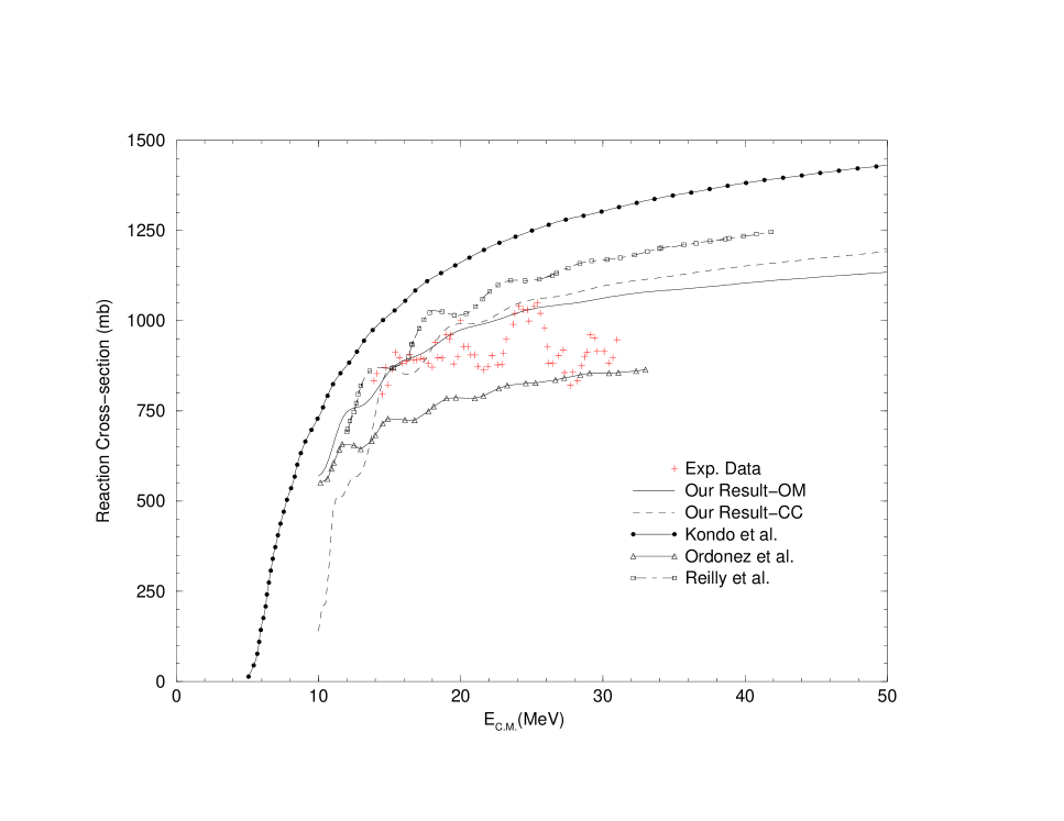
Figure 8: Our reaction cross-section results by using Optical model (solid lines) and Coupled-Channels model (dashed lines) are shown in comparison with the experimental data and other theoretical calculations conducted so far for the same experimental data. The experimental data is taken from [12].

Although these potentials provide good agreement with the experimental data for energies $E/A>6$, the analyses fail for the excitation function and reaction cross-section data at low energies: First of all, in the excitation function analysis, the linearly-energy dependent potential (Equation 6) gives the correct period and phase for the gross oscillations, but the strength is too weak to reproduce the excitation functions at 60⁰ and 80⁰ (ref. [26], Figure 8). The quadratic one (Equation 7) gives a much worse prediction as shown in reference [25], the calculation exactly out of phase with respect to the data for the 90⁰ excitation function. An analysis similar to the work of Brandan et al [25] has also been conducted by Kondo et al [26]. They have modified the UNAM potentials of Brandan et al [25] even further in order to explain 50⁰ to 90⁰ excitation function and reaction cross-section data. Although there are still problems with the strength and phases of the oscillation, an overall explanation of the excitation functions and reaction cross-section data have been provided by this work. Neither Brandan et al [25] nor Kondo et al [26] shows in their paper how good their predictions for the elastic scattering angular distributions are.

Thirdly, Coupled-Channels calculations have been conducted for this reaction. Boztosun and Rae [29] have recently analyzed this reaction over a wide energy range from 32.0 to 126.7 MeV using a new coupling potential. They have added to the usual first-derivative coupling potential with a second-derivative one by considering the orientation of two interacting nuclei and have attempted to solve particularly the magnitude problem of the inelastic mutual-2⁺ state cross-section at high energies. Their approach has provided a good explanation of the elastic and inelastic angular distributions as well as of the excitation functions and has solved the magnitude problem for the inelastic mutual-2⁺ state data, but there are still justification problems regarding the use of such a coupling potential.

In sum, the survey of the literature clearly shows that there is not a potential model that can explain simultaneously the measured elastic scattering angular distribution, the average behavior of the 50⁰ to 90⁰ excitation functions and reaction cross-section data in the low energy region.

In the light of these studies, we have examined the experimental data of ¹²C+¹²C elastic scattering in low and intermediate energy regions. The examination has been conducted in a systematic way in order to find a potential family that simultaneously fits the angular distributions and excitation functions data and to address the problems of this reaction within the framework of the Optical and Coupled-Channels models. 18 individual angular distribution, 5 excitation functions and reaction cross-section data between 32.0 and 70.7 MeV in the laboratory system have been studied, both within the framework of the Optical model and the Coupled-Channels formalism. The experimental data analyzed in this paper is taken from [7, 8, 9, 10, 11, 12].

In the following section, we have introduced our Optical model as well as the potential parameters. In this section, we have first presented the results of the theoretical calculations for the individual angular distributions, 50⁰ to 90⁰ single-angle elastic scattering excitation functions and the reaction cross-section data by using the Optical model and have compared them with the experimental data. We have then provided the volume integrals of the real and imaginary potentials and have discussed their properties in terms of the dispersion relation. In Section 3, we have also introduced our Coupled-Channels model and the results of this analysis are shown for the individual angular distributions, 50⁰ to 90⁰ single-angle elastic scattering excitation functions and the reaction cross-section data. The Optical model and Coupled-Channels calculations have been compared and the effect of including the inelastic channels on the scattering for low energies has been clearly demonstrated. Section 4 is devoted to our summary and conclusion.

2 Optical Model Calculations

In our Optical model analysis, we have used phenomenological complex potentials:

$$V_{nuclear}(r)=\frac{-V}{\left[1+e^{\frac{r-R_{V}}{a_{V}}}\right]^{2}}+i\frac{-W}{1+e^{\frac{r-R_{W}}{a_{W}}}}$$ (1)

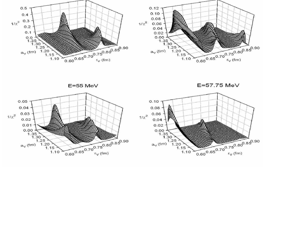
Figure 1: Three-dimensional plots of the optical model parameters $r_{V}$, $a_{V}$ versus 1/$\chi^{2}$, where $\chi^{2}$ has the usual definition and measures the quality of the fit.

Here, $R_{i}$=$r_{i}[A_{P}^{1/3}+A_{T}^{1/3}]$ ($i=V$ or $W$) where $A_{P}^{1/3}$ and $A_{T}^{1/3}$ are the masses of projectile and target nuclei and $r_{V}$ and $r_{W}$ are the radius parameters of the real and imaginary parts of the nuclear potential respectively. The real part of the nuclear potential has the square of the Woods-Saxon shape and the depth ($V$=280.0 MeV) has been fixed to reproduce the experimental data over the whole energy range considered. The experimental data of the ¹²C+¹²C reaction in low energy region has a very oscillatory structure changing very rapidly from energy to energy. Therefore, the radius ($r_{V}$) and diffuseness ($a_{V}$) of the real potential have been varied on a grid, respectively from 0.6 to 0.9 MeV, with steps of 0.01 MeV, and from 1.1 to 1.5 fm with steps of 0.01 fm in order to obtain the best fit to the data. The results of this systematic search are shown in Figure 1 which is a three-dimensional plot of the $r_{V}$, $a_{V}$ and 1/$\chi^{2}$, where $\chi^{2}$ has the usual definition and measures the quality of the fit. In Figure 1, the best fit parameters, producing oscillating cross-sections with reasonable phase and period, correspond to low $\chi^{2}$ values and peaks in the 1/$\chi^{2}$ surface. For the four incident energies, the figures present discrete peaks (or hills) for correlated $r_{V}$ and $a_{V}$ values, which are best fit real potential families and indicate that the $r_{V}$ or $a_{V}$ parameters cannot be varied continuously and still find equally satisfying fits. For the radius ($r_{V}$), the lowest $\chi^{2}$ values are generally obtained between 0.72 and 0.78 and for the diffuseness $a_{V}$, it is between 1.30 and 1.39. Therefore, the radius ($r_{V}$) and diffuseness ($a_{V}$) of the real potential are energy-dependent and the parameters are shown in Table 1. The imaginary part of the nuclear potential given by Equation 1 has been taken as the Woods-Saxon volume form and its depth (W) is given in Table 1. The other parameters of the imaginary potential have also been fixed in the calculations as $r_{W}$=1.1 fm and $a_{W}$=0.55 fm. The real and imaginary parts of the nuclear potential are displayed in Figure 2 for various values of the orbital angular momentum. The Coulomb potential is derived from a uniformly charged sphere with a radius of 5.5 fm.

2.1 Individual Angular Distributions

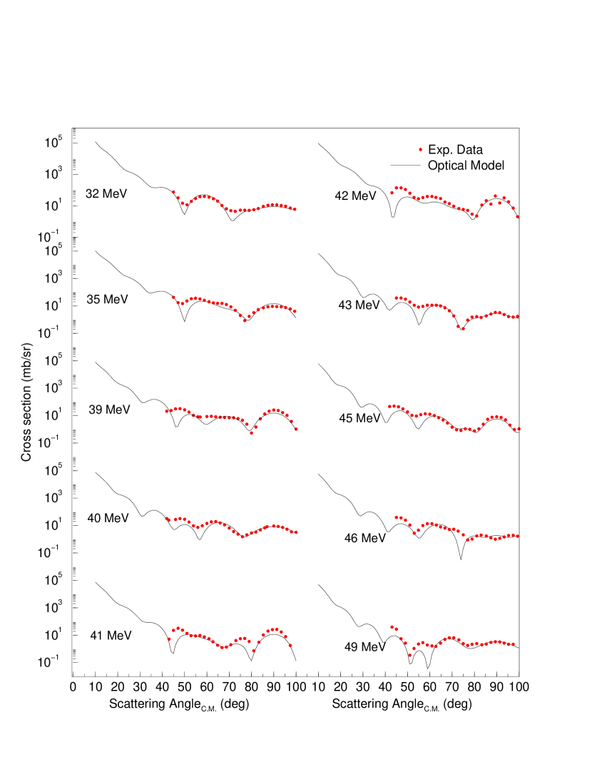
Figure 4: The elastic scattering angular distributions obtained by using the Optical model for the ¹²C+¹²C system. The experimental data is taken from [8].

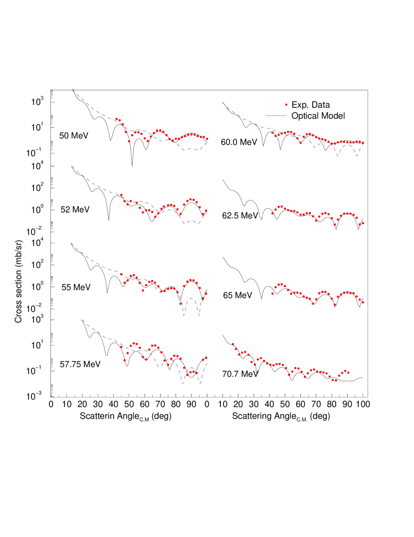
Figure 5: The elastic scattering angular distributions obtained by using the Optical model for the ¹²C+¹²C system (continued from Figure 4). The dashed lines are the angular distributions of the UNAM potential by Brandan et al [25], which is used to explain the excitation functions data at low energies. The experimental data is taken from [8, 10].

We have analyzed 18 angular distributions data measured by references [7, 8, 9, 10] between 32.0 and 70.7 MeV within the above-described Optical potential. The parameters of the real and imaginary potentials as well as $\chi^{2}$ values are given in Table 1. The volume integrals of the potentials are also shown in Table 1 and they are displayed in Figure 3 in comparison with the dispersion relation curve between the real and imaginary parts of the potential. The results of our Optical model calculations (solid lines) are shown in Figures 4 and 5 in comparison with the experimental angular distributions of [7, 8, 9, 10] (circles). As it can be seen from these figures, the places of the maxima and minima in experimental data have been correctly reproduced and there is no magnitude problem between our theoretical predictions and the experimental data. Good agreement between the theoretical calculations and the experimental data has been obtained within the framework of the Optical model. We have also compared our Optical model results with the results of the Brandan et al [25] for 5 energies between 50 and 60 MeV in figure 5. In this figure, the dashed lines are the results of the UNAM potential by Brandan et al [25] which is used to explain the excitation functions data at low energies. Although UNAM potential gives the gross structure of the 90⁰ excitation function, it fails to give a good account of the individual angular distribution at low energies. In the forward angle region up to almost 70⁰ for some energies, the theoretical cross-sections are structureless whereas the experimental cross-section shows oscillatory structure.

2.2 50⁰ to 90⁰ Excitation Functions

It is pointed out in the introduction that the theoretical calculations so far have had limited success in describing the experimental data of this reaction. The potential used to describe the individual angular distributions could not predict the overall behavior of the excitation functions or vice versa. This may be seen from figure 5 for the elastic scattering angular distribution where the dashed-lines are the predictions of UNAM potentials used to explain the excitation functions and reaction cross-section data by Brandan [25] and Kondo et al [26]. Therefore, we have used our potential which fits the individual angular distribution data in order to examine 50⁰ to 90⁰ excitation functions as well as reaction cross-section data. The experimental data of references [9, 10, 11] for the 50⁰, 60⁰, 70⁰, 80⁰ and 90⁰ excitation functions have been analyzed using the parameters of Table 1. In the analysis of individual angular distributions, we have used only 3 free parameters ($r_{V}$, $a_{V}$ and W) within the Optical model and we use now the linear interpolation of the $r_{V}$, $a_{V}$ and W for the excitation function calculations. The reason why we interpolate these parameters is to prevent artificial peaks that might be created by the change of parameters from energy to energy. The linear interpolation of the radius, diffuseness and imaginary potential parameters are

$$r_{V} = 0.80951-0.001226E_{Lab}$$

$$a_{V} = 1.3482-0.00043225E_{Lab}$$

$$W = -0.77098+0.15341E_{Lab}$$ (2)

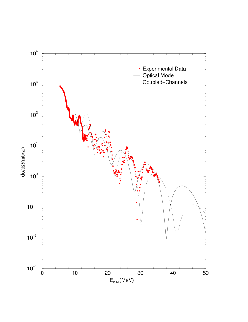
Figure 6: The comparison of the excitation functions of the Optical model prediction (solid lines) and Coupled-Channels prediction (dashed lines) with the experimental data for the 90⁰ elastic scattering excitation function. The experimental data is taken from [10, 11].

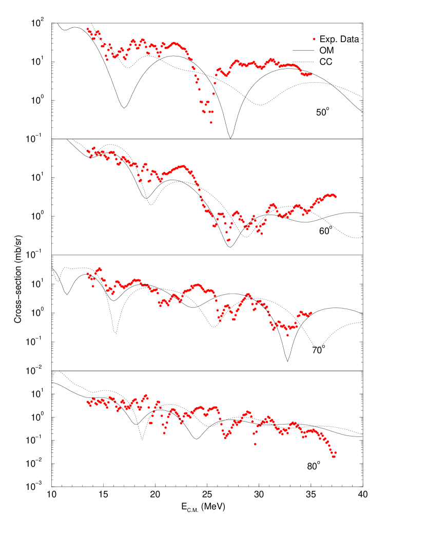
Figure 7: The comparison of the 50⁰, 60⁰, 70⁰ and 80⁰ elastic scattering excitation function results with the experimental data by using the Optical model (solid lines) and Coupled-Channels model (dashed lines). The experimental data is taken from [11].

The results of our Optical model calculations with these interpolations are shown in Figure 6 for the 90⁰ excitation function and in Figure 7 for the other angles. It may be perceived from these figures and the $\chi^{2}$ values in table 3 that the same Optical potentials fitting the individual angular distributions could predict the magnitude of the cross-section correctly and reproduce the period of the gross-structure reasonably well.

2.3 Reaction Cross-section Data

In the same energy region, we have also examined the reaction cross-section data of this reaction by using the same potential parameters i.e. the parameters in Table 1 and Equation 2 for the $r_{V}$, $a_{V}$ and W interpolation. In Figure 8, our reaction cross-section result is shown in comparison with the experimental data as well as with other theoretical calculations conducted so far. We have observed from this figure that our results are in very good agreement with the experimental data; the magnitude and the phases of the oscillations have been correctly provided by our theoretical calculations up to $\sim$ E_Lab=60 MeV. It should be pointed out that our calculations are in better agreement with the experimental data in comparison with the other theoretical calculations conducted so far for the same experimental measurement.

As a result, we have shown in this paper that a potential family could explain 18 individual angular distributions data, 5 excitation functions and reaction cross-sections data simultaneously in a systematic way by using the Optical model. This outcome reveals that our potential belongs to a different family other than the potentials that have been previously used to analyze the experimental data in the higher energy region [25, 26].

In Figure 9, we compare our real potential with the UNAM potentials of Brandan et al [25] and Kondo et al [26] which are successful in describing the high energy data but fail to explain the low energy data. It may be perceived in this figure that our real potential is more diffusive and shallower than their potentials which is a phenomenon distinguishing it from other potentials in the surface region where it is almost half as big as other potentials. Similar differences may be asserted for the imaginary potentials.

The volume integrals and the dispersion relation between the real and imaginary potentials are shown in Figure 3 in comparison with Brandan et al’s potential [25]. The volume integrals of the real and imaginary potentials and the dispersion relation [31] between them have been calculated by using the following formula:

$$J_{V,W}(E)=-\frac{4\pi}{A_{P}A_{T}}\int_{0}^{R}V,W(r,E)r^{2}dr$$ (3)

$$V_{N}(E)=V_{R}+\triangle V(E)=V_{R}-(W/\pi)\left[\varepsilon_{a}ln|\varepsilon_{a}|-\varepsilon_{b}ln|\varepsilon_{b}|\right]$$ (4)

Here $\varepsilon_{i}=(E-E_{i})/(E_{b}-E_{a})$ with $i$ as $a$ and $b$ respectively. The parameters are $E_{a}=32.0$ MeV, $E_{b}=140.0$ MeV, $V_{R}=260.0$ MeV and $W=120.0$ MeV.

We can derive from Figure 3 that the real potential does not obey the dispersion relation at resonance energies observed by Cormier et al [4, 5] for single and mutual-2⁺ states for J=14, 16 and 18 spin values at E_Lab=$\sim 38.0,\sim 50$ and $\sim 57.5$ MeV respectively. In this resonance region, the volume integral of the real potential oscillates remarkably, but the imaginary potential does not accompany the variation of the real one. One explanation of this may be due to the rapid variation of the experimental data, which can not be described by a smoothly varying parameter set and thus, the parameters oscillate. This is also clearly seen from our $\chi^{2}$ search results in Figure 1. For example, the lowest $\chi^{2}$ values for E_lab=50 and 52 MeV in this figure require two very different $r_{V}$ and $a_{V}$ values although there are only $2$ MeV energy difference between two data. It is also possible to interpret that the oscillations in the real potential are manifestations of the coupling to the 2⁺ state, due to the strongly deformed structure of the ¹²C nucleus.

In a previous report [25, 29], the strongly deformed structure of the ¹²C nucleus has been examined and it has been shown that Coupled-Channels calculations with a 20$\%$ decreased imaginary potential of the Optical model calculations have provided an equally good fit to the experimental data. This outcome has shown that the inclusion of the inelastic channels mainly affects the absorption and they have almost no effect in the real part of the nuclear potential in the high energy region for the ¹²C+¹²C system.

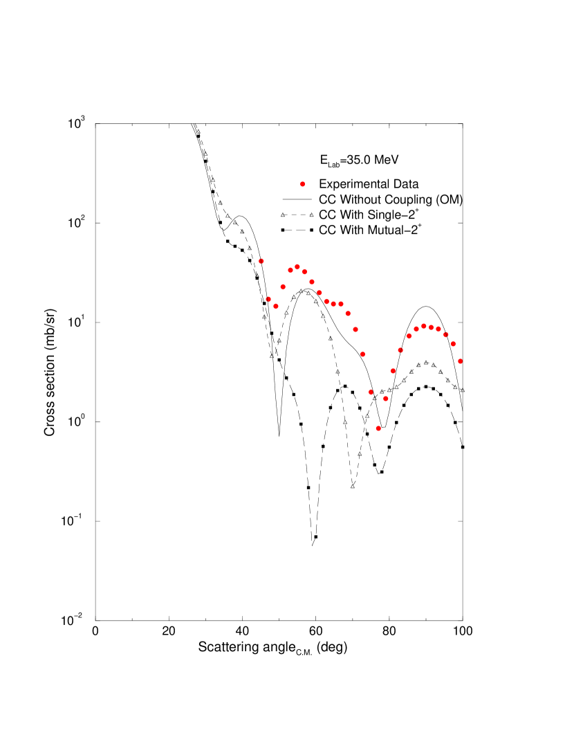
Figure 10: The effect of the inclusion of the single-2⁺ and mutual-2⁺ excited states of the ¹²C nucleus at E_Lab=35.0 MeV. The Optical model parameters of Table 1 are used in the calculations. See the text for the discussion.

However, other previous works such as Sakuragi and Kamimura [32] and references therein have investigated the breakup effect and have shown that the inclusion of the inelastic channels induces a large repulsive real potential. The energies we have studied in this paper are lower than the analysis of ref. [25, 29] and the nature of the experimental data is very different than the nature of those in higher energies. Therefore, it should be questioned how the inclusion of the inelastic channels affects the scattering observables of this reaction. For this purpose, test calculations have been performed at E_Lab=35.0 MeV to see the coupling effect for low energies. In these calculations, we have included the single-2⁺ (4.44 MeV) and mutual-2⁺ (8.88 MeV) states of the strongly deformed ¹²C nucleus. The results of test calculations obtained by using the Optical model parameters as shown in table 1 for E_Lab=35.0 MeV are displayed in Figure 10.

Test runs with and without coupling (i.e. Optical model) at E_Lab=35.0 MeV have, however, shown striking differences. As shown in Figure 10, the inclusion of the excited states at E_Lab=35.0 MeV has very large effects not only in backward, but also in forward-angle regions ($\theta_{C.M.}\leq 40^{0}$). The coupling changes the magnitudes and phases of the oscillations in the cross-section. We have infered from this effect that the coupling not only affects the absorptive or imaginary part, but also the real part of the nuclear potential. As a result, it modifies the interference between incoming and outgoing waves, which creates the oscillatory structure in the cross-section. Our findings are in agreement with the observation of Sakuragi and Kamimura [32]. Therefore, according to this outcome, the claim of ref. [25] that is the inclusion of the inelastic channels mainly affects the absorption and they have almost no effect in the real part of the nuclear potential in the high energies is not valid for the low energy region the ¹²C+¹²C system.

3 Coupled-Channels Calculations

Having seen the coupling effect, we conduct Coupled-Channels calculation for the same energies considered in Optical model calculations. In the Coupled-Channels calculations, the interaction between the ¹²C nuclei is described by a deformed Optical potential. The real potential has the square of a Woods-Saxon shape as in Equation 1 with a depth of 280 MeV. The other parameters, as shown in Table 2, have been fitted to reproduce the elastic scattering data. The imaginary potential has the standard Woods-Saxon volume shape as in Equation 1 and the parameters of its depth are given in Table 2. The radius and diffuseness of the imaginary potential have been fixed in the calculations as $r_{W}$=1.1 fm and $a_{W}$=0.55 fm.

It has been assumed that the target nucleus ¹²C has a static quadrupole deformation and this assumption has been taken into account by deforming the real potential in the following way:

$$R(\theta,\phi)=r_{0}A_{p}^{1/3}[1+\beta_{2}Y_{20}(\theta,\phi)]+r_{0}A_{t}^{1/3}[1+\beta_{2}Y_{20}(\theta,\phi)]$$ (5)

where the first and second terms account for the projectile and target excitations respectively. In equation 5, $\beta_{2}$=-0.6 is the deformation parameter of the ¹²C nucleus. This value is derived from its known B(E2) value, which is 42 e${}^{2}fm^{4}$ [33]. We have noticed that deformation of the imaginary part of the nuclear potential does not have any significant effect. Thus, for computational simplicity, we have not deformed it in the present Coupled-Channels calculations. An extensively modified version of the code Chuck and the code Fresco has been used both in the Optical model and Coupled-Channels calculations [34, 35].

3.1 Individual Angular Distributions

Using this Coupled-Channels model, we have analyzed the same experimental data as in the case of the Optical model. The parameters of the real and imaginary potentials as well as their volume integrals are given in Table 2. The volume integrals are also displayed in figure 3 in comparison with the volume integrals of the Optical model potentials and the dispersion relation curve obtained by using equation 4.

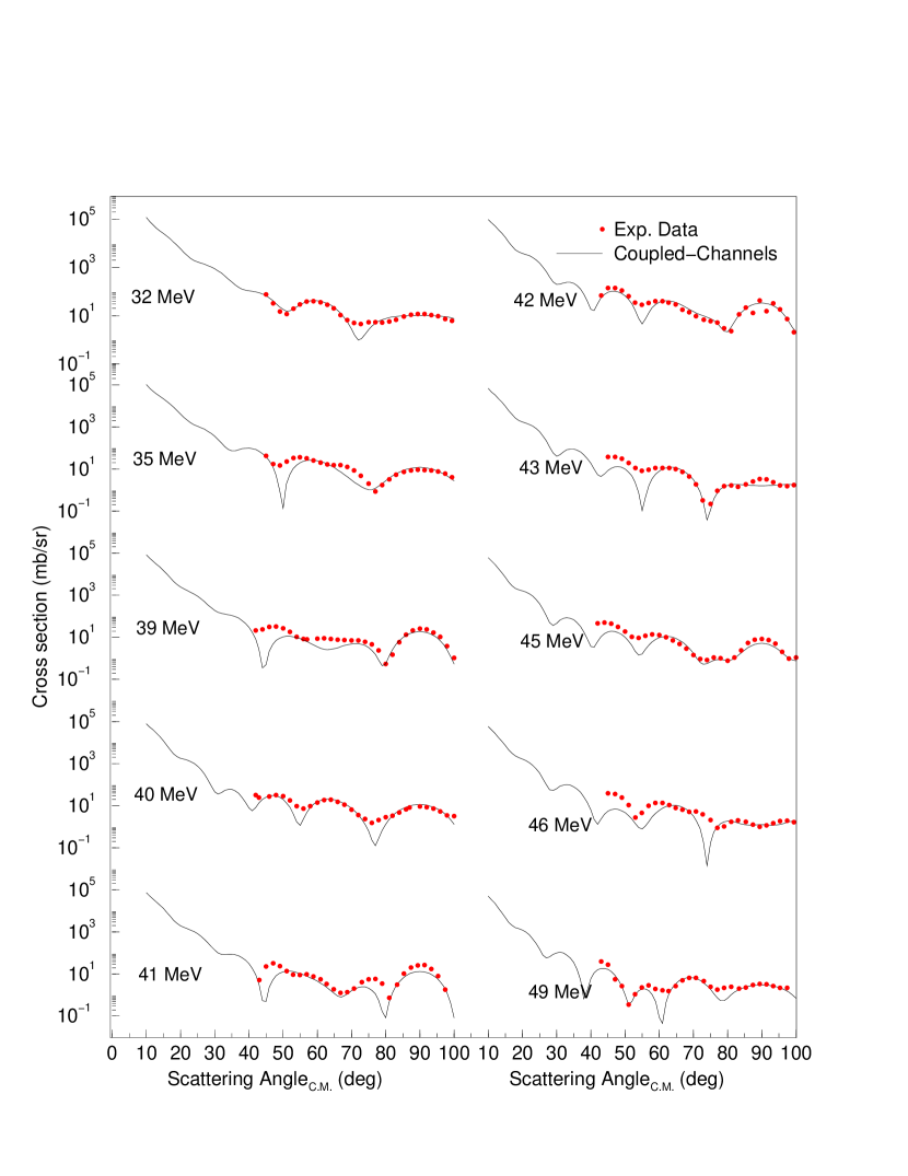
Figure 11: The elastic scattering angular distributions obtained by using the Coupled-Channels model for the ¹²C+¹²C system. The experimental data is taken from [8].

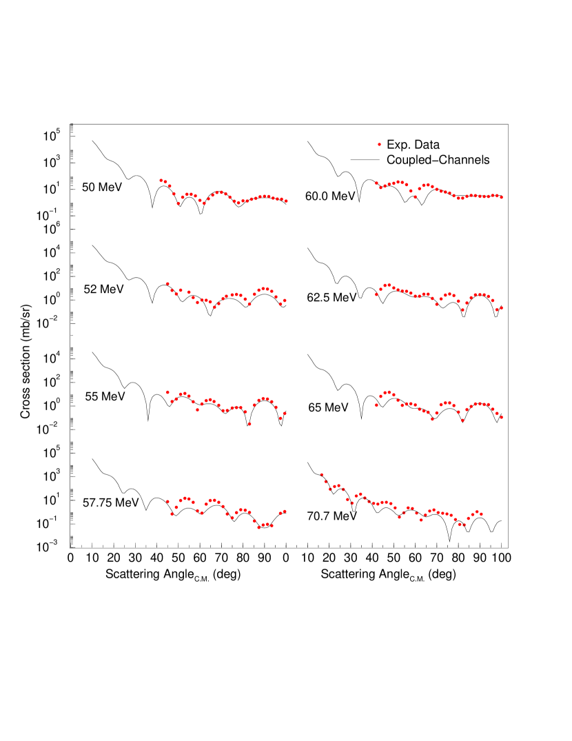
Figure 12: The elastic scattering angular distributions obtained by using the Coupled-Channels model for the ¹²C+¹²C system (continued from Figure 11). The experimental data is taken from [8, 10].

The results of our Coupled-Channels calculations (solid lines) are shown in Figures 11 and 12 in comparison with the experimental data (circles). As it can be seen from these figures and the $\chi^{2}$ values in Table 2, reasonable agreement between the theoretical calculations and the experimental data has been obtained. The phases and magnitudes of the oscillations have been predicted correctly for the energies considered.

The effect of the inclusion of the single-2⁺ state of the ¹²C nucleus in Coupled-Channels calculations should be underlined here. The effect of the Coupled-Channels calculations has been very large on the scattering and its effect has been clearly observed in our theoretical calculations for the cross-section at forward, intermediate and large angles. It has changed the phases and magnitudes of the oscillations at all angles. In order to obtain the agreement between theoretical calculations and experimental data, we have had to change not only the imaginary part, but also the real part of the nuclear potential. As seen in figure 3, the inclusion of the single-2⁺ state has reduced the strength of the imaginary potential at all energies in comparison with the imaginary potential of the Optical model. This reduction of the imaginary potential was expected since the Coupled-Channels calculations take into account the effect of the eliminated channels of the Optical model. However, the coupling has had a big effect on the real potential and has changed the strength of the real potential very much. This remarkable change of the real potential parameters has been due to the coupling between ground and single-2⁺ states and in contrast with the observations at high energies. At high energies, the coupling does not change the phase of the oscillations and therefore, reducing the imaginary potential would be enough to obtain Optical model results. We should state that this strong coupling effect should be taken into account in the analysis in order to gain a better description of the nuclear potential in the interaction of such strongly deformed two nuclei.

3.2 50⁰ to 90⁰ Excitation Functions and Reaction Cross-section Data

We have also analyzed the 50⁰ to 90⁰ excitation functions as well as reaction cross-section data. We have used linear interpolation of 3 free parameters given in Table 2, i.e. $r_{V}$, $a_{V}$ and W, as follows:

$$r_{V} = 0.78664-0.00056643E_{Lab}$$

$$a_{V} = 1.3476+0.00073848E_{Lab}$$

$$W = -4.1719+0.209E_{Lab}$$ (6)

The results for the 90⁰ excitation function are shown in Figure 6, for the other angles in Figure 7, and for the reaction cross-section data in Figure 8 in comparison with the Optical model results and experimental data. Again reasonable agreement with the experimental data both for the excitation functions and for the reaction cross-section data has been obtained within the framework of the Coupled-Channels method. However, we should point out that the Optical model results for the excitation function calculations are in better agreement with the experimental data as it can be seen from the $\chi^{2}$ values in Table 3. For the reaction cross-section, the Coupled-Channels results are better than the Optical model results at low energies, but towards high energies our Coupled-Channels calculations have over-estimated the data. It is higher than the experimental data and Optical model results. This discrepancy arises due to the interpolation formulae given in equation 6 for $r_{V}$, $a_{V}$ and W. Second or third-order interpolations of the parameters in Table 2 have provided a better result for the excitation functions and reaction cross-section data.

3.3 Resonances

In this section, we give the prediction of our potential for the well-known resonances measured by Cormier et al. [4, 5] for the single-2⁺ state. These resonances observed at low energies could not be predicted by a potential, which also fits the angular distributions and the excitation functions. We show the predictions of our potential in Figure 13. In the upper part of this figure, we display the real versus the imaginary part of the S-matrix for the resonance spin values J=14, J=16 and J=18 and in the lower part of the figure we show the magnitudes of the S-matrix ($|S_{L}|$) for the elastic ($0^{+}-0^{+}$) and single-$2^{+}$ ($0^{+}-2^{+}$) channels against the center of mass energy for the same spin values. Our potential predict the places of the resonances at the correct energies with reasonable widths.

4 Summary and Conclusion

We provide a consistent description of the elastic scattering of the ¹²C+¹²C system from 32.0 to 70.7 MeV in the laboratory system by using a phenomenological, strongly attractive Woods-Saxon squared nuclear potential, with a relatively weak absorption, with both the Optical model and Coupled-Channels formalism. This reaction has been one of the most extensively studied reaction over the last forty years, in particular, in the low energy region where an oscillatory structure in the excitation functions and resonances observed has been pronounced. Unfortunately, no global model has been set forth so far that consistently explains the measured experimental data over a wide energy range. In the introduction, we present the problems that this reaction manifests, one of the most important of which is the simultaneous description of the elastic scattering angular distributions and the single-angle excitation functions data. The theoretical calculations in the past have reported that a potential family that fits the individual angular distributions is unable to reproduce the excitation functions data of the same reaction in a systematic way.

By considering these problems, we analyze this reaction with available experimental data in the energy range we considered and show that it is possible to improve the agreement for the individual angular distributions, excitation functions and the reaction cross-section data simultaneously with a deep real and shallow imaginary potential. From our analysis, we observe that away from the resonance energies, the variation of the potential parameters has a systematic energy-dependence as in the case of the high energy region. However, when there is a rapid variation of the experimental data, it can not be described by a smoothly varying parameter set and thus, the parameters oscillate. In our analysis, we observe this effect. It should be underlined here that the remarkable success of our potential in explaining the individual angular distributions, excitation functions and the reaction cross-section data simultaneously is achieved by using only 3 free parameters ($r_{V}$, $a_{V}$ and $W$) in the calculations.

We should also point out that the coupling between ground and excited states has a large effect on the scattering in the low energy region. The inclusion of the excited states of the ¹²C nucleus at E_Lab=35.0 MeV alters the places and magnitudes of oscillations at both forward and backward angles around 90⁰ in the theoretical results. That means, the coupling not only changes the absorptive part of the nuclear potential, but also the real part of the nuclear potential which is in agreement with the microscopic calculations of Sakuragi and Kamimura [32]. Our results show that at low energies, the Coupled-Channels effect should be explicitly taken into account for strongly deformed nuclei such as ¹²C. At high energies, we observe that the inclusion of the excited states does not change the phases of the oscillation but affects the magnitude of the cross-section at large angles. We do not observe effects at forward angles. No effect on the phases of the oscillations means that the inclusion of the excited states has almost no effect on the real part of the nuclear potential. The effect at large angles can also be compensated by decreasing the absorptive part of the nuclear potential. This outcome is in agreement with previous claims [25, 29], but valid only at high energies.

The deep real potential used in our Optical and Coupled-Channels analysis has a different radial shape, separating it from other potentials used in the analysis of the higher energy data ($E/A\geq 6$ MeV). Both Optical and Coupled-Channels potentials in our analysis provide very good fits to the elastic scattering angular distributions and reasonable improvement to the 50⁰ to 90⁰ excitation functions and reaction cross-section data. It also predicts the resonances at the correct energies with reasonable widths. To our knowledge, this has not been achieved for the ¹²C+ ¹²C reaction at low energies so far.

This work is supported by the Turkish Science and Research Council (TÜBİTAK), Grant No: TBAG-2398 and Erciyes University-Institute of Science: Grant no: FBA-03-27, FBT-04-15, FBT-04-16.

$E_{Lab}$	$r_{V}$	$a_{V}$	$W$	$J_{V}$	$J_{W}$	$\chi^{2}$
MeV	fm	fm	MeV	MeV.fm3	MeV.fm3
32.0	0.78	1.39	4.2	296.5	17.4	2.51
35.0	0.77	1.33	4.7	281.2	19.5	4.74
39.0	0.78	1.33	5.2	290.7	21.6	6.32
40.0	0.77	1.37	5.0	285.0	20.8	4.19
41.0	0.72	1.39	5.0	242.9	20.8	5.62
42.0	0.73	1.35	5.5	247.5	22.8	7.72
43.0	0.76	1.39	6.2	277.7	25.8	3.62
45.0	0.76	1.39	6.2	277.7	25.8	4.59
46.0	0.78	1.33	6.5	290.7	27.0	6.36
49.0	0.73	1.39	6.0	251.3	24.9	5.58
50.0	0.74	1.39	6.4	259.9	26.6	4.95
52.0	0.78	1.39	8.5	296.5	35.3	9.88
55.0	0.81	1.30	9.0	318.1	37.3	5.95
57.75	0.76	1.39	8.9	277.7	37.0	8.65
60.0	0.74	1.33	8.0	254.2	33.3	5.52
62.5	0.74	1.39	8.0	259.9	33.3	9.55
65.0	0.72	1.33	8.9	237.3	37.0	15.79
70.7	0.715	1.39	12.0	238.8	49.9	16.14

Table 1: The parameters and the volume integrals of the real and imaginary potentials as well as the $\chi^{2}$ values of the Optical model calculations. Coulomb radius, $r_{c}$=1.2 fm.

$E_{Lab}$	$r_{V}$	$a_{V}$	$W$	$J_{V}$	$J_{W}$	$\chi^{2}$
MeV	fm	fm	MeV	MeV.fm3	MeV.fm3
32.0	0.76	1.30	3.2	269.3	13.3	2.19
35.0	0.74	1.37	3.2	257.9	13.3	4.53
39.0	0.78	1.38	3.2	295.5	13.3	5.76
40.0	0.81	1.39	3.5	326.5	14.5	4.15
41.0	0.69	1.45	4.2	225.1	17.4	5.58
42.0	0.81	1.35	4.9	322.6	20.4	6.77
43.0	0.74	1.42	5.3	262.9	22.0	4.97
45.0	0.74	1.45	5.2	266.0	21.6	4.88
46.0	0.76	1.37	5.6	275.7	23.2	6.92
49.0	0.80	1.33	5.7	310.5	23.7	3.74
50.0	0.80	1.32	5.8	309.6	24.1	3.64
52.0	0.739	1.39	7.7	259.0	32.0	11.94
55.0	0.79	1.37	8.0	304.3	33.2	7.14
57.75	0.74	1.45	8.3	266.0	34.5	8.49
60.0	0.77	1.38	8.0	286.0	33.2	6.32
62.5	0.72	1.45	7.7	249.0	32.0	8.36
65.0	0.70	1.39	8.1	226.9	33.6	11.86
70.7	0.77	1.35	12.0	283.0	49.9	13.59

Table 2: The parameters and the volume integrals of the real and imaginary potentials as well as the $\chi^{2}$ values of the Coupled-Channels calculations. Coulomb radius, $r_{c}$=1.2fm.

$\theta_{C.M.}$	$50^{0}$	$60^{0}$	$70^{0}$	$80^{0}$	$90^{0}$
OM (Eq. 2)	40.16	4.44	26.82	67.15	31.96
CC (Eq. 5)	51.07	16.29	36.44	183.3	112.3

Table 3: $\chi^{2}$ values of the 50⁰ to 90⁰ excitation functions by using the Optical and Coupled-Channels models.

Figure 2: The interaction potential between ¹²C and ¹²C is plotted against the separation R for various values of the orbital angular momentum quantum number, $l$. The inserted figure shows our imaginary potential at $E_{Lab}$=32.0 MeV and 70.7 MeV. The parameters are given in the text.

Figure 3: The volume integrals of the real and imaginary parts of the nuclear potential used in the Optical model (filled and empty squares) and Coupled-Channels calculations (filled and empty circles). Here, the filled and empty triangles are the volume integrals of Brandan et al’s potentials [25] and the solid and dashed lines are the dispersion relation between real and imaginary components of the nuclear potential calculated by using equation 4.

Figure 9: The comparison of our nuclear potential, used in the Optical model calculations, with the Brandan et al’s [25] and Kondo et al’s [26] nuclear potentials used in the analysis of the experimental data at high energies (E/A$\geq$6).

Figure 13: Resonances: In the upper part of the figure, we show the real versus imaginary part of the S-Matrix for the spin values J=14, J=16 and J=18 and in the lower part, the magnitudes of the S-matrix ($|S_{L}|$) for the elastic ($0^{+}-0^{+}$) and single-$2^{+}$ ($0^{+}-2^{+}$) channels against the center of mass energy for the same spin values.

References

- [1] D.A. Bromley, J.A. Kuehner and E. Almquist, Phys. Rev. Lett. 4 (1960) 365.
- [2] E. Almquist, D.A. Bromley and J.A. Kuehner and , Phys. Rev. Lett. 4 (1960) 515.
- [3] K.A. Erb and D.A. Bromley, Phys. Rev. C 23 (1981) 2781.
- [4] T.M. Cormier, J. Applegate, G.M. Berkowitz, P. Braun-Munzinger, P.M. Cormier, J.W. Harris, C.M. Jachcinski, L. Lee, J. Barrette and H.E. Wegner, Phys. Rev. Lett. 38 (1977) 940.
- [5] T.M. Cormier, C.M. Jachinski, G.M. Berkowitz, P. Braun-Munzinger, P.M. Cormier, M. Gai, J.W. Harris, J. Barrette and H.E. Wegner, Phys. Rev. Lett. 40 (1978) 924.
- [6] B.R. Fulton, T.M. Cormier and B.J. Herman, Phys. Rev. C21 (1980) 198.
- [7] E.R. Cosman, T.M. Cormier, K. Van Bibber, A. Sperduto, G. Young, J. Erskine, L.R. Greenwood and O. Hansen, Phys. Rev. Lett 35 (1975) 265.
- [8] E.R. Cosman, R. Ledoux, and A.J. Lazzarini, Phys. Rev. C 21 (1980) 2111.
- [9] R.G. Stokstad, R.M. Wieland, C.B. Fulmer, D.C. Hensley, S. Raman, A.H. Snell and P.H. Stelson, Oak Ridge National Laboratory, Report No. ORNL/TM-5935, 1977 (Unpublished).
- [10] R.G. Stokstad, R.M. Wieland, G.R. Satchler, C.B. Fulmer, D.C. Hensley, S. Raman, L.D. Rickertsen, A.H. Snell and P.H. Stelson, Phys. Rev. C 20 (1979) 655.
- [11] A. Morsad, F. Haas, C. Beck, and R.M. Freeman, Z. Phys. A338 (1979) 61.
- [12] J.J.Kolata, R.M. Freeman, F. Haas, B. Heusch and A. Gallman, Phys. Rev. C 21 (1980) 579.
- [13] K.A. Erb and D.A. Bromley, in Treatise on Heavy-Ion Science, Vol. 3, ed. D.A. Bromley (Plenum, New York, 1985).
-
[14]
W. Greiner, J.Y. Park, W. Scheid, Nuclear Molecules (World-Scientific, Singapore
1995).
G.R. Satchler, Direct Nuclear Reactions (Oxford Uni. Press, Oxford 1983).
H. Feshbach, Theoretical Nuclear Physics: Nuclear Reactions (Wiley, NewYork 1992). - [15] M.E. Brandan and G.R. Satchler, Phys. Rep. 285 (1997) 143.
-
[16]
M. Freer, M.P. Nicoli, S.M. Singer, C.A. Bremner, S.P.G. Chappell, W.D.M. Rae,
I. Boztosun, B.R. Fulton, D.L. Watson, B.J. Greenhalgh, G.K. Dillon,
R.L. Cowin and D.C. Weisser, Phys. Rev. C70(2004) 064311.
C.A. Bremner, S.P.G. Chappell, W.D.M. Rae, I. Boztosun, M. Freer, M.P. Nicoli, S.M. Singer, B. Fulton, D.L. Watson, B.J. Greenhalgh, G.K. Dillon, R.L. Cowin, Phys. Rev. C66 (2002) 034605. - [17] S. Marsh, and W.D.M. Rae, Phys. Lett. 180B (1986) 185.
- [18] H. Flocard, P.H. Heenen, S.J. Krieger, and M.S. Weiss, Prog. Theor. Phys. 72(1984) 1000.
- [19] C.E. Ordoñez, R.J. Ledoux and E.R. Cosman, Phys. Lett. 173B (1986) 39.
- [20] Y. Kondo, Y. Abe and T. Matsuse, Phys. Rev. C 19 (1979) 1356.
- [21] Y.Abe, Y. Kondo and T. Matsuse, Suppl. Prog. Theor. Phys. 68 (1980) 303.
- [22] T. Matsuse, Y. Abe, Y. Kondo, Prog. Theor. Phys. 59 (1978) 1904.
- [23] A. Morsad, F. Haas, C. Beck, and R.M. Freeman, Z. Phys 338 (1991) 61.
- [24] N. Rowley, H. Doubre, C. Marty, Phys. Letts. 69B (1997) 147.
- [25] M.E. Brandan, M. Rodriguez-Villafuerte and A. Ayala, Phys. Rev. C 41 (1990) 1520.
- [26] Y. Kondō, M.E. Brandan and G.R. Satchler, Nucl. Phys. A637 (1998) 175.
- [27] K.W. McVoy and M.E. Brandan, Nucl. Phys. A542 (1992) 295.
- [28] M.E. Brandan, M.S. Hussein, K.W. McVoy and G.R. Satchler, Comments Nucl. Part. Phys. 22 (1996) 77.
-
[29]
I. Boztosun and W.D.M Rae, Phys. Rev. C 63 (2001) 054607.
I. Boztosun and W.D.M. Rae, Phys. Lett. 518B (2001)229. - [30] F Michel and S. Ohkubo, Eur. Phys. J. A19 (2004) 333.
- [31] G.R. Satchler, Phys. Rep. 199 (1991) 147.
-
[32]
Y. Sakuragi and M. Kamimura, Phys. Lett. 149B (1984)
307.
Y. Sakuragi, M. Yahiro and M. Kamimura, Prog. Theor. Phys. 70 (1983) 1047.
M. Ito, Y. Sakuragi and Y. Hirabayashi, Phys. Rev. C 63, 064303 (2001).
Y. Sakuragi, M. Ito, M. Katsuma, M. Takashina, Y. Kudo, Y. Hirabayashi, S. Okabe, and Y. Abe, in Proceedings of the 7th International Conference on Clustering Aspects of Nuclear Structure and Dynamics, edited by M. Korolija, Z. Basrak, and R. Caplar (World Scientific, Singapore, 2000), p. 138. -
[33]
R.H. Stelson and L. Grodzins, Nucl. data 1A (1966) 21.
F. Ajzenberg-Selove, Nucl. Phys. A248 (1975) 1. - [34] P.D. Kunz, CHUCK, a Coupled-Channels code, unpublished.
-
[35]
I.J. Thompson, FRESCO, a Coupled-Channels code, unpublished.
I.J. Thompson, Computer Physics Reports 7 (1988) 167.