Isospin violation in the vector form factors of the nucleon

Abstract

A quantitative understanding of isospin violation is an increasingly important ingredient for the extraction of the nucleon’s strange vector form factors from experimental data. We calculate the isospin violating electric and magnetic form factors in chiral perturbation theory to leading and next-to-leading order respectively, and we extract the low-energy constants from resonance saturation. Uncertainties are dominated largely by limitations in the current knowledge of some vector meson couplings. The resulting bounds on isospin violation are sufficiently precise to be of value to on-going experimental studies of the strange form factors.

I Introduction

Since a nucleon has no valence strange quarks, the strange form factors provide information about the dynamics of virtual quarks within a nucleon. In recent years the strange electric and magnetic form factors have been studied experimentally by the SAMPLE Spayde et al. (2004), A4 Maas et al. (2004, 2005), HAPPEX Aniol et al. (2006, 2005), and G0 Armstrong et al. (2005) Collaborations, and theoretically via lattice QCD simulations Dong et al. (1998); Mathur and Dong (2001); Lewis et al. (2003); Leinweber et al. (2005a, b, 2006), chiral perturbation theory Musolf and Ito (1997); Hemmert et al. (1998, 1999); Hammer et al. (2003); Kubis (2005), and hadron models Silva et al. (2004, 2005); Jido and Weise (2005); Carvalho et al. (2005); Chen et al. (2004); Bijker (2005); An et al. (2006); Riska and Zou (2005). (For a discussion of earlier theoretical studies, see Ref. Ramsey-Musolf (2005).) A central conclusion of recent research is that the strange electric and magnetic form factors are small, perhaps even small enough to require a careful understanding of the competing effects from isospin violation.

The inequality of up and down quarks, in terms of both mass and electric charge, produces effects that mimic the strange form factors. Extraction of the authentic strange quark effects from experimental data requires this isospin violation to be understood theoretically. There have been a number of theoretical studies of isospin violation in this context Dmitrasinovic and Pollock (1995); Miller (1998); Lewis and Mobed (1999a); Ma (1997); Thomas et al. (2005), but it is not yet clear that uncertainties in these results are negligible with respect to the strange form factors. Refs. Dmitrasinovic and Pollock (1995); Miller (1998) used quark model discussions to determine the isospin violating contributions, and found them to be less than 1%; in fact the strange magnetic form factor received no contribution at all for vanishing momentum transfer. This null contribution at $Q^{2}=0$ is not due to any symmetry of QCD, and therefore the chiral perturbation theory (ChPT) study in Ref. Lewis and Mobed (1999a) did find a non-zero contribution, but it includes an undetermined low-energy constant. One could think of extracting the physics of this constant, for example, from the light-cone baryon model of Ref. Ma (1997) or from the quark model approach of Ref. Gardner et al. (1996), though it is difficult to see how to match these models to the consistent low-energy effective theory description of ChPT in order to avoid double counting problems.

In the present work we address two main goals. First we revisit the calculation of chiral loops, this time using both a manifestly covariant formalism Becher and Leutwyler (1999) and heavy-baryon ChPT. We find that the two formalisms offer complementary advantages for various aspects of this calculation. Since the isospin violating effects begin at rather high orders in the chiral expansion, leading order (LO) $={\cal O}(p^{4})$ and next-to-leading order (NLO) $={\cal O}(p^{5})$ (where $p$ collectively stands for small parameters like momenta, the pion mass, or the electric coupling), the cross-check of the entire calculation in both formalisms is valuable, and we are able to identify and correct some errors in Ref. Lewis and Mobed (1999a).

Our second major goal in the present work is to estimate the lone combination of low-energy constants that appears in the chiral perturbation theory expressions. For this, we employ resonance saturation. The physics producing isospin violation in the nucleon’s vector form factors is seen to be $\rho$–$\omega$ mixing, and numerical values for the required vector meson couplings are obtained from recent dispersive analyses.

A question that cannot be fully answered by our work relates to the convergence of the chiral expansion. With only LO and NLO results, it is impossible to make any definitive statement about convergence. A completely consistent extension beyond NLO seems unwarranted, since it would involve two-loop integrals and would introduce additional unknown low-energy constants. However, given the apparent smallness of the strange form factors and of the isospin violating form factors, we can neglect contributions that are simultaneously isospin violating and strange. This allows the discussion of isospin violation to occur within two-flavor ChPT, where convergence properties are known to be dramatically better than for the three-flavor theory.

The present work thus provides a complete discussion of the physics at LO for the electric and at NLO for the magnetic isospin violating form factors, producing numerical values for isospin violation in the magnetic moment, electric radius, and magnetic radius, which are of direct relevance to the ongoing experimental studies of strange form factors.

The outline of our presentation is as follows. We define the form factors under consideration and their leading moments in Section II. The chiral representation of the Dirac form factors to leading order and of the Pauli form factors to next-to-leading order is (re-)derived in some detail in Section III. In order to provide resonance-saturation estimates for unknown chiral low-energy constants, we calculate the contributions of $\rho$–$\omega$ mixing in Section IV, which also allow for some insight into higher-order contributions beyond what is strictly calculated in ChPT. The pertinent formalism to do this consistently with chiral constraints is included. We conclude our findings in Section V. Some technical details are relegated to the appendices.

II Basic Definitions

We define the isospin symmetry breaking Dirac and Pauli form factors according to

$$\begin{split}\bigl{\langle}p(\vec{p}\,^{\prime})&+n(\vec{p}\,^{\prime})\,\bigl{|}\,\frac{1}{2}\bigl{(}\bar{u}\gamma_{\mu}u-\bar{d}\gamma_{\mu}d\bigr{)}\,\bigr{|}\,p(\vec{p})+n(\vec{p})\bigr{\rangle}\\ &=~{}\bar{u}(p^{\prime})\Bigl{[}\gamma_{\mu}{F_{1}^{\!\not\,v}}(t)+\frac{i\sigma_{\mu\nu}q^{\nu}}{2m_{N}}{F_{2}^{\!\not\,v}}(t)\Bigr{]}u(p)~{},\\ \bigl{\langle}p(\vec{p}\,^{\prime})&-n(\vec{p}\,^{\prime})\,\bigl{|}\,\frac{1}{6}\bigl{(}\bar{u}\gamma_{\mu}u+\bar{d}\gamma_{\mu}d\bigr{)}\,\bigr{|}\,p(\vec{p})+n(\vec{p})\bigr{\rangle}\\ &=~{}\bar{u}(p^{\prime})\Bigl{[}\gamma_{\mu}{F_{1}^{\!\not\,s}}(t)+\frac{i\sigma_{\mu\nu}q^{\nu}}{2m_{N}}{F_{2}^{\!\not\,s}}(t)\Bigr{]}u(p)~{},\end{split}$$ (1)

where $q_{\mu}=p^{\prime}_{\mu}-p_{\mu}$, $t=q^{2}$. $\!\not\!\!\!v$, $\!\not\!\!\!s$ refer to isospin breaking pieces in the isovector and isoscalar vector currents, respectively. Our notation is linked to that used in Refs. Dmitrasinovic and Pollock (1995); Lewis and Mobed (1999a) by

$${F_{i}^{\!\not\,v}}(t)={{}^{u-d}F_{i}^{p+n}}(t)~{},\quad{F_{i}^{\!\not\,s}}(t)={{}^{u+d}F_{i}^{p-n}}(t)~{}.$$

The Sachs form factors are defined in terms of these as

$$\begin{split}{G_{E}^{\!\not\,v,\not\,s}}(t)&={F_{1}^{\!\not\,v,\not\,s}}(t)+\frac{t}{4m_{N}^{2}}{F_{2}^{\!\not\,v,\not\,s}}(t)~{},\\ {G_{M}^{\!\not\,v,\not\,s}}(t)&={F_{1}^{\!\not\,v,\not\,s}}(t)+{F_{2}^{\!\not\,v,\not\,s}}(t)~{}.\end{split}$$ (2)

Current conservation implies ${F_{1}^{\!\not\,v,\not\,s}}(0)=0$, while the Pauli form factors are normalized to the isospin breaking pieces of the (anomalous) magnetic moments,

$${F_{2}^{\!\not\,v,\not\,s}}(0)~{}=~{}{\kappa^{\!\not\,v,\not\,s}}~{}.$$ (3)

To complete the definition of the leading moments of these form factors, we define radius-like terms as the coefficients of form factor terms linear in $t$,

$$\begin{split}{F_{1/2}^{\!\not\,v,\not\,s}}(t)&={F_{1/2}^{\!\not\,v,\not\,s}}(0)+{\rho_{1/2}^{\!\not\,v,\not\,s}}\,t+{\cal O}(t^{2})~{},\\ {G_{E/M}^{\!\not\,v,\not\,s}}(t)&={G_{E/M}^{\!\not\,v,\not\,s}}(0)+{\rho_{E/M}^{\!\not\,v,\not\,s}}\,t+{\cal O}(t^{2})~{}.\end{split}$$ (4)

Finally, the proton’s neutral weak form factors $G_{E/M}^{p,Z}$ depend on one specific linear combination of isospin breaking form factors,

$$\begin{split}G_{E/M}^{p,Z}(t)=&\,\bigl{(}1-4\sin^{2}\theta_{W}\bigr{)}G_{E/M}^{p}(t)-G_{E/M}^{n}(t)\\ &-G_{E/M}^{s}(t)-G_{E/M}^{u,d}(t)~{},\end{split}$$ (5)

where $\theta_{W}$ is the weak mixing angle, $G_{E/M}^{s}(t)$ are the strange vector form factors, and

$$G_{E/M}^{u,d}(t)\doteq{G_{E/M}^{\!\not\,s}}(t)-{G_{E/M}^{\!\not\,v}}(t)~{}.$$ (6)

We will use an analogous notation also for the leading moments, i.e. $\kappa^{u,d}={\kappa^{\!\not\,s}}-{\kappa^{\!\not\,v}}$ etc. Eq. (5) demonstrates that the isospin breaking form factors “simulate” strangeness form factors even in a world without strange quarks Lewis and Mobed (1999a, b), such that they have a direct impact on the accuracy to which the strangeness form factors can be extracted from data.

III Chiral Perturbation Theory

III.1 Effective Lagrangians

We have performed the relevant loop calculations both in the heavy-baryon formalism Jenkins and Manohar (1991); Bernard et al. (1995) and in the infrared regularization scheme of relativistic baryon ChPT Becher and Leutwyler (1999). For reasons of briefness, we only display the relativistic forms of the relevant Lagrangian terms in this section. The equivalent heavy-baryon forms can be found in the quoted references.

The Goldstone boson (pion) Lagrangian is given, at leading order, by

$${\cal L}_{\pi\pi}^{(2)}=\frac{F^{2}}{4}\langle u_{\mu}u^{\mu}+\chi_{+}\rangle~{},$$ (7)

where the matrices $u^{2}=U$ collect the pion fields in the usual manner, $u_{\mu}=iu^{\dagger}\nabla_{\mu}Uu^{\dagger}$ with the covariant derivative $\nabla_{\mu}$. The field $\chi_{+}=u^{\dagger}\chi u^{\dagger}+u\chi^{\dagger}u$ contains the quark mass terms, $\chi=2B\,\text{diag}(m_{u},m_{d})+\ldots$, where $B$ is linked to the quark condensate in the chiral limit, and $F$ can be identified with the pion decay constant, $F=F_{\pi}=92.4$ MeV. $\langle\ldots\rangle$ denotes the trace in flavor space.

A striking observation is the fact that the leading term generating the charged-to-neutral pion mass difference Ecker et al. (1989a),

$${\cal L}_{\pi\pi\gamma^{*}}^{(2)}=ZF^{4}\langle Q_{+}^{2}-Q_{-}^{2}\rangle~{}\Rightarrow~{}M_{\pi^{+}}^{2}-M_{\pi^{0}}^{2}=2Ze^{2}F^{2}~{},$$

where $Q_{\pm}=\frac{1}{2}(uQu^{\dagger}\pm u^{\dagger}Qu)$, $Q=\text{diag}(e,0)$, does not feature in the following calculation: in nuclear physics language, this operator only breaks charge independence (independence under completely general rotations in isospin space), but not charge symmetry (rotations by $\pi$ about a fixed axis in isospin space, resulting in the simultaneous exchange of $u$ and $d$ quarks, as well as protons and neutrons) as required for the form factors in Eq. (1), so the pion mass difference alone will never generate contributions to the form factors under investigation, and we will neglect terms that are of second order in isospin breaking.

The leading-order pion-nucleon Lagrangian is given by

$${\cal L}_{\pi N}^{(1)}=\bar{\Psi}\Bigl{\{}i\!\not\!\!D-m+\frac{g_{A}}{2}\!\not\!u\gamma_{5}\Bigr{\}}\Psi~{},$$ (8)

where $D_{\mu}$ is the usual covariant derivative acting on the nucleon, $m$ is the nucleon mass in the chiral limit, and $g_{A}$ can be identified with the axial coupling constant, $g_{A}=1.26$. Of the second-order pion-nucleon Lagrangian (that also contains all possible effects of virtual photons), we only quote the terms relevant for our calculation:

$$\begin{split}{\cal L}_{\pi N\gamma^{*}}^{(2)}=\bar{\Psi}\Bigl{\{}&c_{5}\tilde{\chi}_{+}+f_{2}F^{2}\langle Q_{+}\rangle Q_{+}\\ &+\frac{\sigma^{\mu\nu}}{8m}\bigl{(}c_{6}F^{+}_{\mu\nu}+c_{7}\langle F^{+}_{\mu\nu}\rangle\bigr{)}\Bigr{\}}\Psi~{}.\end{split}$$ (9)

Here we have introduced the notation $\tilde{O}=O-\frac{1}{2}\langle O\rangle$ for traceless operators. $F_{\mu\nu}^{+}=u^{\dagger}F_{\mu\nu}u+uF_{\mu\nu}u^{\dagger}$ contains the usual electromagnetic field strength tensor. There are two types of terms in Eq. (9): $c_{6}$ and $c_{7}$ are related to the isovector and isoscalar anomalous magnetic moments (in the chiral limit) according to

$$\kappa^{v}=\kappa_{p}-\kappa_{n}=c_{6}~{},\quad\kappa^{s}=\kappa_{p}+\kappa_{n}=c_{6}+2c_{7}~{},$$ (10)

with the experimental values $\kappa^{v}=3.706$, $\kappa^{s}=-0.120$, while the operators proportional to $c_{5}$ and $f_{2}$ generate the leading proton-neutron mass difference

$$\Delta m\doteq m_{n}-m_{p}=4B(m_{u}-m_{d})c_{5}+e^{2}F^{2}f_{2}~{}.$$ (11)

As all our results will be expressible in terms of $\Delta m$, we do not have to care about the precise separation of this mass difference into its strong ($\propto c_{5}$) and electromagnetic ($\propto f_{2}$) parts. We have neglected to spell out terms in Eq. (9) that lead only to a common nucleon mass shift and can be taken care of by replacing the nucleon mass in the chiral limit by its physical value, $m\to m_{N}=\frac{1}{2}(m_{p}+m_{n})$.

Finally, the following fourth-order terms Fettes et al. (2000); Müller and Meißner (1999) contribute to the isospin breaking form factors:

$$\begin{split}{\cal L}_{\pi N{\gamma^{*}}}^{(4)}&=\bar{\Psi}\Bigl{\{}-\frac{e_{107}}{2}\langle F_{\mu\nu}^{+}\rangle\tilde{\chi}_{+}-\frac{e_{108}}{2}\langle\tilde{F}_{\mu\nu}^{+}\tilde{\chi}_{+}\rangle\\ &\qquad+h_{40}F^{2}\langle Q_{+}\rangle\langle\tilde{Q}_{+}\tilde{F}_{\mu\nu}^{+}\rangle\\ &\qquad+h_{43}F^{2}\langle Q_{+}\rangle\tilde{Q}_{+}\langle F_{\mu\nu}^{+}\rangle\Bigr{\}}\sigma^{\mu\nu}\Psi\,.\end{split}$$ (12)

The terms proportional to $e_{107}$, $h_{43}$ contribute to ${\kappa^{\!\not\,s}}$, the terms multiplied by $e_{108}$, $h_{40}$ to ${\kappa^{\!\not\,v}}$. Therefore, both form factors contain one counterterm each proportional to $m_{u}-m_{d}$ and $e^{2}$. The constants $e_{108}$, $h_{40}$ contain a divergent piece,

$$e_{108}=e^{r}_{108}(\lambda)+\beta_{e_{108}}L~{},\quad h_{40}=h^{r}_{40}(\lambda)+\beta_{h_{40}}L~{},$$

where $L$ has a pole in $(d-4)$,

$$L=\frac{\lambda^{d-4}}{16\pi^{2}}\biggl{\{}\frac{1}{d-4}+\frac{1}{2}\bigl{[}\gamma_{E}-1-\log 4\pi\bigr{]}\biggr{\}}~{},$$

$\lambda$ is the dimensional regularization scale, and $\gamma_{E}$ is Euler’s constant. The scale-dependent finite constants $e^{r}_{108}$, $h^{r}_{40}$ obey a renormalization group equation according to

$$\lambda\frac{d}{d\lambda}e^{r}_{108}(\lambda)=-\frac{\beta_{e_{108}}}{16\pi^{2}}~{},\quad\lambda\frac{d}{d\lambda}h^{r}_{40}(\lambda)=-\frac{\beta_{h_{40}}}{16\pi^{2}}~{}.$$

In order to render the isospin breaking magnetic moments finite and scale-independent, we find the beta functions

$$\beta_{e_{108}}=\frac{2g_{A}^{2}c_{5}}{F^{2}}~{},\qquad\beta_{h_{40}}=-\frac{g_{A}^{2}f_{2}}{F^{2}}~{}.$$

In contrast, $e_{107}$ and $h_{43}$ are finite and scale-independent.

It should be mentioned that Ref. Lewis and Mobed (1999a) included the $\Delta(1232)$ as an explicit field in ChPT. When the corresponding loop diagrams were computed, their momentum dependences were found to be negligible relative to the final error bands on the form factors. Since these effects would also be insignificant relative to the error bands that will be obtained in the present work, we omit the explicit $\Delta(1232)$ field from the outset. In the framework used here, its effects would show up via higher-order low-energy constants that are beyond the accuracy we aim at in this work.

III.2 Power counting

We repeat here some power counting arguments that were mostly already put forward in Ref. Lewis and Mobed (1999a).

It is easy to see that the usual (isospin conserving) vector form factors receive polynomial contributions to the leading moments, i.e. magnetic moment, electric (or Dirac) radius, magnetic (or Pauli) radius, at chiral orders $p^{2}$, $p^{3}$, $p^{4}$, respectively. Pion loop contributions start at ${\cal O}(p^{3})$, therefore such loop effects can generate a parameter-free leading-order prediction for the magnetic radius. The leading magnetic radius term has to scale like $M_{\pi}^{-1}$; this infrared singularity has been well-known for a long time Bég and Zepeda (1972).

Figure 1: One-pion-loop diagrams. Full/dashed/wiggly lines denote nucleons/pions/vector currents, respectively. The filled circles in diagrams (d) and (e) represent the magnetic couplings from ${\cal L}_{\pi N\gamma^{*}}^{(2)}$. The crossed diagrams of (c) and (e) are not depicted separately. Mass insertions on the nucleon propagator lines, yielding the physical proton and neutron masses, are not explicitly shown.

From the previous section, it is obvious that polynomial contributions to the leading moments of the isospin violating form factors always have to include factors of either $m_{u}-m_{d}$ or $e^{2}$, therefore they are suppressed by two orders in the chiral power counting with respect to the isospin conserving ones. We therefore find precisely the terms of ${\cal L}_{\pi N\gamma^{*}}^{(4)}$ in Eq. (12) contributing to the magnetic moments, while operators of electric and magnetic radius type would arise at orders $p^{5}$ and $p^{6}$. On the other hand, the pion loop diagrams with additional mass insertions of the $c_{5}$, $f_{2}$ operators in Eq. (9), shown in Fig. 1, start to contribute only one order higher than the same diagrams without mass corrections, therefore leading loop contributions are also of order $p^{4}$. This means that, while a prediction of the isospin violating magnetic moments is hampered by the a priori unknown ${\cal L}_{\pi N\gamma^{*}}^{(4)}$ counterterms, both electric and magnetic radii can be unambiguously predicted at leading order, and for the magnetic radii even the next-to-leading-order corrections are free of unknown parameters. The leading infrared singularity in the magnetic radius scales like $\Delta m/M_{\pi}^{2}$, the leading electric and subleading magnetic radius terms like $\Delta m/M_{\pi}$.

Figure 2: A pair of two-loop diagrams. The closed wiggly lines denote virtual photons. The sum of both contributions to the magnetic form factor drops out.

A calculation of the isospin violating Pauli (or magnetic) form factor up to ${\cal O}(p^{5})$ is massively facilitated by the fact that no two-loop diagrams contribute. This can be seen as follows:

1. As mentioned in Section III.1, the pion mass difference alone cannot generate charge symmetry breaking terms. Therefore, diagrams with two pion loops would require another (subleading) charge symmetry breaking vertex or the nucleon mass difference in order to contribute, which would then, however, be at least of order $p^{6}$.

2. Two photon loops are of second order in isospin breaking and can be disregarded. In addition, it is easily seen in the heavy-baryon formalism that such diagrams with only leading-order photon couplings cannot generate the spin operators necessary for a magnetic contribution.

3. Finally, there might be diagrams with one pion and one photon loop. The only diagrams that generate a magnetic structure at ${\cal O}(p^{5})$ are of the type (a) in Fig. 1, with one additional photon loop attached. However, it can be checked in the heavy-baryon formulation that the sum of the two diagrams in Fig. 2 is proportional to the anticommutator of the two Pauli–Lubanski spin operators stemming from the pion-nucleon couplings, and therefore it again only yields a contribution to the electric form factor. The same mechanism can be checked for all other possible diagrams.

Furthermore, also one-loop diagrams with isospin-breaking vertices (other than the nucleon mass difference insertion) can be ruled out of consideration:

1. Tadpole graphs with isospin breaking couplings fail to generate infrared singularities proportional to $M_{\pi}^{-1}$.

2. The third-order pion-nucleon Lagrangian contains isospin breaking pion-nucleon coupling constants. However, these affect only the $\pi^{0}NN$ coupling, hence they do not contribute in a type (a) diagram, while the remaining diagrams in Fig. 1 are subleading in their contributions to the Pauli form factor and therefore can only play a role at ${\cal O}(p^{6})$.

Figure 3: One-photon-loop diagrams with magnetic couplings. The sum of both diagrams vanishes. (The addition of a crossed right diagram is implied.)

Finally, the only one-photon loops contributing to the magnetic form factor are the ones depicted in Fig. 3. They have no $t$-dependence up to the chiral order considered here, and it is easily calculated that their contribution to $F_{2}(0)$ exactly cancels.

Therefore we have proven that the only infrared singular contributions to the charge symmetry breaking form factor radii, and all contributions up to ${\cal O}(p^{4})$ for the Dirac and up to ${\cal O}(p^{5})$ for Pauli form factor in addition to the ${\cal L}_{\pi N\gamma^{*}}^{(4)}$ counterterms in Eq. (12), are given by nucleon mass difference effects in the diagrams in Fig. 1.

III.3 Chiral representation of the form factors

In this section, we write down the chiral representations of the charge-symmetry breaking form factors, the Dirac form factors to leading order, the Pauli form factors up to next-to-leading order. We decompose all form factors according to

$${F_{1/2}^{\!\not\,v,\not\,s}}(t)\doteq{F_{1/2}^{\!\not\,v,\not\,s}}(0)+{\bar{F}_{1/2}^{\!\not\,v,\not\,s}}(t)~{},$$ (13)

where current conservation dictates

$${F_{1}^{\!\not\,v}}(0)={F_{1}^{\!\not\,s}}(0)=0~{}.$$

For convenience, we define an overall dimensionless prefactor

$$C=\frac{g_{A}^{2}m_{N}\Delta m}{(4\pi F_{\pi})^{2}}\approx 1.4\times 10^{-3}~{}.$$ (14)

Then the $t$-independent terms of the Pauli form factors are given by

$$\begin{split}{F_{2}^{\!\not\,v}}(0)&=4C\biggl{[}1+2\log\frac{M_{\pi}}{\lambda}-\frac{\pi(\kappa^{v}+6)M_{\pi}}{2m_{N}}\biggr{]}\\ &+8m_{N}\Bigl{[}e^{2}F^{2}h^{r}_{40}-2B(m_{u}-m_{d})e^{r}_{108}\Bigr{]}~{},\\ {F_{2}^{\!\not\,s}}(0)&=-4C\,\frac{\pi(\kappa^{s}+1)M_{\pi}}{m_{N}}\\ &+8m_{N}\Bigl{[}e^{2}F^{2}h_{43}-2B(m_{u}-m_{d})e_{107}\Bigr{]}~{}.\end{split}$$ (15)

Altogether, we find for the ultimately required combination

$$G_{M}^{u,d}(0) = {F_{2}^{\!\not\,s}}(0)-{F_{2}^{\!\not\,v}}(0)$$ (16)

$$= -4C\bigg{[}1+2\log\frac{M_{\pi}}{\lambda}+\frac{\pi(2\kappa^{s}-\kappa^{v}-4)M_{\pi}}{2m_{N}}\biggr{]}$$

$$+\kappa_{CT}^{u,d}~{},$$

where

$$\kappa_{CT}^{u,d}=8m_{N}\!\Bigl{[}e^{2}F^{2}\bigl{(}h_{43}-h^{r}_{40}\bigr{)}-2B(m_{u}-m_{d})\bigl{(}e_{107}-e^{r}_{108}\bigr{)}\Bigr{]}.$$ (17)

Note that in order to ease notation, we have suppressed the scale dependence of $h^{r}_{40}$, $e^{r}_{108}$, $\kappa_{CT}^{u,d}$ in Eqs. (15)–(17) that is necessary to compensate for the chiral logarithms.

Up to the order we are considering, the chiral representations of the form factors ${F_{1/2}^{\!\not\,s}}(t)$ display no $t$-dependence,

$${\bar{F}_{1}^{\!\not\,s}}(t)={\bar{F}_{2}^{\!\not\,s}}(t)=0~{}.$$ (18)

This is due to the fact that only diagram (a) in Fig. 1 contains a two-pion-cut and therefore generates momentum dependence in the low-energy region, and that the isoscalar vector current does not couple to pions at this order. The $t$-dependence of the form factors ${F_{i}^{\!\not\,v}}(t)$, on the other hand, is given unambiguously in terms of pion loop contributions and can be written as

$${\bar{F}_{1}^{\!\not\,v}}(t) = -\frac{2g_{A}^{2}M_{\pi}\Delta m}{F_{\pi}^{2}}\Bigl{[}\bar{\gamma}_{0}(t)-4\bar{\gamma}_{3}(t)\Bigr{]}~{},$$ (19)

$${\bar{F}_{2}^{\!\not\,v}}(t) = -\frac{4g_{A}^{2}m_{N}\Delta m}{F_{\pi}^{2}}$$ (20)

$$\times\biggl{(}\xi(t)-\frac{M_{\pi}}{m_{N}}\Bigl{[}\bar{\gamma}_{0}(t)-5\bar{\gamma}_{3}(t)\Bigr{]}\biggr{)}~{}.$$

The explicit representations of the loop functions $\xi(t)$, $\bar{\gamma}_{0/3}(t)$ are given in Appendix A.1. We note that the corresponding expressions reported in Ref. Lewis and Mobed (1999a) contain errors: Eqs. (53) and (54) in that work are too large by factors of 2 and 4 respectively; Eqs. (19) and (20) of the present work are the correct expressions, and we have obtained them separately from heavy-baryon ChPT and from infrared regularization. Expanding the loop functions to linear order in $t$, we find the radius term according to

$$\begin{split}{\rho_{M}^{u,d}}&=\frac{2C}{3M_{\pi}^{2}}\biggl{[}1+\frac{5\pi M_{\pi}}{4m_{N}}-\frac{3\pi M_{\pi}}{m_{N}}\biggr{]}\\ &=\frac{2C}{3M_{\pi}^{2}}\biggl{[}1-\frac{7\pi M_{\pi}}{4m_{N}}\biggr{]}~{},\end{split}$$ (21)

where the first correction stems from ${F_{1}^{\!\not\,v}}(t)$ and the second from the subleading terms in ${F_{2}^{\!\not\,v}}(t)$. Numerically, we find that, due to the large enhancement factor of $7\pi/4\approx 5.5$, the next-to-leading-order correction reduces the leading prediction for the magnetic radius term by as much as 80%.

IV Contributions from $\rho$–$\omega$ mixing

The missing ingredient in order to make the chiral representations of the previous section predictive is a value for the counterterm combination $\kappa_{CT}^{u,d}$ that is unconstrained from symmetry arguments. As no phenomenological information is available to fix these constants, we have to resort to model estimates in order to get a handle on them. The obvious model to use seems to be resonance saturation.

The method to estimate chiral low-energy constants by including heavier resonance fields in the theory and matching their low-energy limit to higher-order operators was first introduced systematically in the context of meson ChPT in Refs. Ecker et al. (1989a, b); Donoghue et al. (1989). It was shown to work rather well for the constants in ${\cal L}_{\pi\pi}^{(4)}$, in particular, those constants that receive contributions from vector and axial vector resonances were shown to be numerically dominated by these (a modern version of the concept of “vector meson dominance”).

In Ref. Bernard et al. (1997) this method was extended to the pion-nucleon sector, nucleon resonances (in particular the $\Delta(1232)$) were included, and it was demonstrated that most of the constants in ${\cal L}_{\pi N}^{(2)}$ can also be well understood this way. However little is known about how well this procedure works for higher-order pion-nucleon coupling constants. In Ref. Kubis and Meißner (2001a) it was found for the nucleon vector form factors that in particular the isovector couplings are not well saturated by the $\rho$ contribution alone. This observation agrees with the results of various dispersive analyses of these form factors (see e.g. Refs. Höhler et al. (1976); Mergell et al. (1996); Hammer and Meißner (2004)) that always require several resonances per channel in order to describe the data adequately.

Despite this rather pessimistic view, there is reason to believe that resonance saturation for the isospin violating vector form factors might in principle work better than for the isospin conserving ones; we will comment on this point again at the end of Section IV.2. The only resonances that can contribute at tree level are vector mesons, and isospin violation is provided by the well-known mixing of the isovector $\rho^{0}$ and the isoscalar $\omega$ state. We lay out the formalism for incorporating vector mesons, their mixing and coupling to vector currents and nucleons in the following section before presenting analytical and numerical results for the isospin violating magnetic moments. Contributions to the higher moments (electric and magnetic radii) will come as a benefit that allows us to estimate higher-order corrections to the leading chiral loop predictions.

IV.1 Formalism, Lagrangians

We here discuss the necessary ingredients to describe the interaction of vector mesons with external currents as well as nucleons. We make use of the antisymmetric tensor formulation that was shown to be particularly useful in the context of ChPT and resonance saturation investigations Ecker et al. (1989a, b). Most of the literature is concerned with vector mesons in the context of SU(3) ChPT; we will here only be concerned with the SU(2) subsystem and adapt the formalism accordingly. In SU(2), the antisymmetric tensor $V_{\mu\nu}$ is given in terms of $\rho$ and $\omega$ fields according to

$$V_{\mu\nu}=\frac{1}{\sqrt{2}}\bigl{(}\vec{\rho}_{\mu\nu}\cdot\vec{\tau}+\omega_{\mu\nu}\bigr{)}~{}.$$

The free Lagrangian for $V_{\mu\nu}$ then takes the form

$${\cal L}_{V}=-\frac{1}{2}\langle D^{\mu}V_{\mu\nu}D_{\rho}V^{\rho\nu}\rangle+\frac{M_{V}^{2}}{4}\langle V_{\mu\nu}V^{\mu\nu}\rangle~{}.$$ (22)

In particular, Eq. (22) leads to a common vector meson mass $M_{\rho}=M_{\omega}=M_{V}$. For numerical results, we will use the mass of the $\rho$, $M_{V}=770$ MeV. The coupling of the vector mesons to external vector (and axial vector) sources is given by

$${\cal L}_{V\gamma}=\frac{F_{V}}{2\sqrt{2}}\langle V^{\mu\nu}{\cal F}^{+}_{\mu\nu}\rangle~{},$$ (23)

where ${\cal F}^{+}_{\mu\nu}$ contains the electromagnetic field strength tensor proportional to the quark charge matrix $\mathcal{Q}=e/3\,\text{diag}(2,-1)$ (as opposed to the nucleon charge matrix $Q$ used elsewhere in this text). Eq. (23) correctly reproduces the SU(3) relation for the vector meson decay constants $F_{\rho}=3F_{\omega}=F_{V}$. Phenomenologically, this relation is rather well fulfilled, $F_{\rho}=152.5$ MeV, $F_{\omega}=45.7$ MeV.

Mixing of $\rho^{0}$ and $\omega$ has been discussed in a formalism similar to the one presented here in Ref. Urech (1995), albeit in the framework of SU(3). Here, we perform an analogous construction for SU(2). We are not interested in (isospin-conserving) quark mass renormalization effects of the vector meson masses, but only in terms contributing to $\rho$–$\omega$ mixing. One single such term can be constructed,

$${\cal L}_{mix}=\frac{v_{mix}}{8}\langle V_{\mu\nu}\rangle\langle\tilde{V}^{\mu\nu}\chi_{+}\rangle~{},$$ (24)

where we have once more made use of the notation $\tilde{V}_{\mu\nu}=V_{\mu\nu}-\frac{1}{2}\langle V_{\mu\nu}\rangle$. If we match Eq. (24) to the SU(3) result in Ref. Urech (1995), also invoking quark counting rules Gasser and Leutwyler (1982), the mixing parameter can be identified with $v_{mix}=2M_{V}/B$. In addition, there is a $\rho$–$\omega$ transition through an intermediate photon via the interaction term Eq. (23). Combining both effects, one finds the on-shell mixing amplitude

$$\Theta_{\rho\omega}=2M_{V}(m_{u}-m_{d})+\frac{e^{2}F_{V}^{2}}{3}~{}.$$ (25)

The latest analysis of experimental data Kucurkarslan and Meißner (2006) yields

$$\Theta_{\rho\omega}=(-3.75\pm 0.36)\times 10^{-3}~{}\text{GeV}^{2}~{},$$ (26)

well in agreement with earlier numbers Urech (1995).

The coupling of vector mesons to baryons, formulated in the antisymmetric tensor formalism, was discussed in Ref. Borasoy and Meißner (1996). The relation of the generic couplings used in that reference to the more conventional vector and tensor couplings was given in Ref. Kubis and Meißner (2001a). For a more compact presentation, we rewrite the terms from Ref. Borasoy and Meißner (1996) in a SU(2) form, employing immediately standard couplings, which results in

$$\begin{split}{\cal L}_{VN}&=-\frac{M_{V}}{\sqrt{2}}\bar{\Psi}\biggl{[}\frac{\sigma^{\mu\nu}}{4m_{N}}\Bigl{\{}g_{\rho}\kappa_{\rho}\tilde{V}_{\mu\nu}+\frac{g_{\omega}\kappa_{\omega}}{2}\langle V_{\mu\nu}\rangle\Bigr{\}}\\ &+\frac{\gamma^{\mu}}{M_{V}^{2}}\Bigl{\{}g_{\rho}\bigl{[}D^{\nu},\tilde{V}_{\mu\nu}\bigr{]}+\frac{g_{\omega}}{2}\bigl{[}D^{\nu},\langle V_{\mu\nu}\rangle\bigr{]}\Bigr{\}}\biggr{]}\Psi~{}.\end{split}$$ (27)

We remark here that we totally neglect $\rho$–$\phi$ mixing in this analysis (which would be present at least in an SU(3) extension). Although the $\phi$–nucleon couplings are not as small as the Zweig rule might lead one to expect, see e.g. Refs. Mergell et al. (1996); Hammer and Meißner (2004), the mixing is roughly an order of magnitude smaller than that between $\rho$ and $\omega$ Bijnens and Gosdzinsky (1996); Benayoun and O’Connell (2001), and therefore beyond the accuracy we aim to achieve by this model estimate.

IV.2 Analytical results

Figure 4: The two diagrams involving $\rho$–$\omega$ mixing that contribute to the isospin breaking form factors. The double lines denote vector meson propagators, the cross represents the mixing vertex.

The $\rho$–$\omega$ mixing contributions to the isospin violating Dirac and Pauli form factors can be derived from the two diagrams depicted in Fig. 4. They are given in terms of the various coupling constants defined in the previous section as follows:

$$\begin{split}{F_{1}^{\!\not\,v}}(t)\,\Bigr{|}_{mix}&=-\frac{g_{\omega}F_{\rho}\,\Theta_{\rho\omega}\,t}{M_{V}(M_{V}^{2}-t)^{2}}~{},\\ {F_{1}^{\!\not\,s}}(t)\,\Bigr{|}_{mix}&=-\frac{g_{\rho}F_{\omega}\,\Theta_{\rho\omega}\,t}{M_{V}(M_{V}^{2}-t)^{2}}~{},\\ {F_{2}^{\!\not\,v}}(t)\,\Bigr{|}_{mix}&=-\frac{g_{\omega}\kappa_{\omega}F_{\rho}\,M_{V}\,\Theta_{\rho\omega}}{(M_{V}^{2}-t)^{2}}~{},\\ {F_{2}^{\!\not\,s}}(t)\,\Bigr{|}_{mix}&=-\frac{g_{\rho}\kappa_{\rho}F_{\omega}\,M_{V}\,\Theta_{\rho\omega}}{(M_{V}^{2}-t)^{2}}~{}.\end{split}$$ (28)

From these, one can easily derive the leading moments:

$$\begin{split}\kappa^{u,d}_{mix}&=\bigl{(}g_{\omega}\kappa_{\omega}F_{\rho}-g_{\rho}\kappa_{\rho}F_{\omega}\bigr{)}\frac{\Theta_{\rho\omega}}{M_{V}^{3}}~{},\\ \bigl{(}\rho_{1}^{u,d}\bigr{)}_{mix}&=\bigl{(}g_{\omega}F_{\rho}-g_{\rho}F_{\omega}\bigr{)}\frac{\Theta_{\rho\omega}}{M_{V}^{5}}~{},\\ \bigl{(}\rho_{2}^{u,d}\bigr{)}_{mix}&=\bigl{(}g_{\omega}\kappa_{\omega}F_{\rho}-g_{\rho}\kappa_{\rho}F_{\omega}\bigr{)}\frac{2\Theta_{\rho\omega}}{M_{V}^{5}}~{}.\end{split}$$ (29)

For the phenomenological discussion, we will be even more interested in the leading moments of the Sachs form factors, which are given in terms of the above as

$$\begin{split}{\rho_{E}^{u,d}}&={\rho_{1}^{u,d}}+\frac{\kappa^{u,d}}{4m_{N}^{2}}~{},\\ {\rho_{M}^{u,d}}&={\rho_{1}^{u,d}}+{\rho_{2}^{u,d}}~{}.\end{split}$$ (30)

In light of the above results, we want to comment on the claim made earlier that the saturation of coupling constants by vector meson contributions might work better here than for the isospin conserving form factors considered in Ref. Kubis and Meißner (2001a). The reason is that the additional propagator in the mixing case leads to a higher power of vector meson masses in the denominators of the leading moments, Eq. (29). A heavier pair of isovector and isoscalar vector resonances sufficiently close to each other in mass to mix, e.g. the $\rho(1450)$ and the $\omega(1420)$ Eidelman et al. (2004), would yield contributions of the same form as Eq. (29), but suppressed by a higher power of mass ratios $M_{V^{\prime}}/M_{V}\approx 2$ than their unmixed contributions to the conventional form factors.

Finally, we want to comment on the possibility of isospin violation other than through mixing. In particular, it is possible to construct a mechanism for “direct” isospin breaking in the vector-meson–nucleon couplings in analogy to Eq. (12),

$${\cal L}_{VN}^{u,d}~{}\propto~{}\bar{\Psi}\,\sigma^{\mu\nu}\Bigl{\{}e_{\rho}\langle\tilde{V}_{\mu\nu}\tilde{\chi}_{+}\rangle+e_{\omega}\langle V_{\mu\nu}\rangle\tilde{\chi}_{+}\Bigr{\}}\Psi~{},$$

which results in the $\rho$ coupling as an isoscalar and the $\omega$ coupling as an isovector to the nucleons. (Analogous terms with the charge instead of the quark mass matrix are easily written down.) We disregard this possibility for the reason that the vector-meson–nucleon coupling strengths are extracted from dispersive analyses on the assumption of isospin symmetry (with the exception of $\rho$–$\omega$ mixing in the isovector spectral function), i.e. the $\omega$ couplings, for instance, are identified as certain pole strengths in the isoscalar channel. In this way, an isospin breaking $\rho$-nucleon coupling would just be taken as part of the $\omega$ resonance, and vice versa.

IV.3 Numerical results

The couplings of the vector mesons to nucleons are a rather delicate issue and we prefer to rely as directly as possible on data rather than on models. To this end, we concentrate on values extracted from dispersive analyses of electromagnetic form factors of the nucleon, and disregard values extracted from meson exchange models of nucleon-nucleon scattering or pion-photo-/electroproduction (see e.g. Refs. Machleidt et al. (1987); Stoks et al. (1994); Davidson et al. (1991); Pasquini et al. (2006)). As it is well known that pure vector meson dominance does not yield an adequate description of the isovector spectral function, where the two-pion continuum leads to a significant enhancement on the left shoulder of the $\rho$ peak Bernard et al. (1996), more recent analyses Mergell et al. (1996); Mergell (1995); Hammer and Meißner (2004); Belushkin et al. (2006) make use of the full pion form factor plus $\pi\pi\to N\bar{N}$ partial waves. In order to approximately disentangle the spectral function from Ref. Belushkin et al. (2006) into a non-resonant two-pion continuum plus a $\rho$ contribution, we follow the method of Ref. Kaiser (2003) and add a Breit–Wigner parameterization of the $\rho$ resonance to either the chiral one-loop or the two-loop Kaiser (2003) representation of the two-pion cut contributions. This decomposition is model dependent, but probably adequate for a model estimate of low-energy constants.

Table 1: $\rho$–nucleon coupling constants and corresponding form factor contributions. “1-loop” and “2-loop” refer to the part of the non-resonant two-pion continuum that has been used to extract the $\rho$ couplings. For details, see main text.

	Ref. Mergell et al. (1996); Mergell (1995)	Ref. Belushkin et al. (2006) + 1-loop	Ref. Belushkin et al. (2006) + 2-loop
$g_{\rho}$	4.0	5.4	6.2
$\kappa_{\rho}$	6.1	6.8	5.1
$10^{2}\times{\kappa^{\!\not\,s}}$	0.9	1.4	1.2
$10^{2}\times\frac{{\kappa^{\!\not\,s}}}{4m_{N}^{2}}~{}\bigl{[}{\rm GeV}^{-2}\bigr{]}$	0.3	0.4	0.3
$10^{2}\times{\rho_{1}^{\!\not\,s}}~{}\bigl{[}{\rm GeV}^{-2}\bigr{]}$	0.3	0.3	0.4
$10^{2}\times{\rho_{2}^{\!\not\,s}}~{}\bigl{[}{\rm GeV}^{-2}\bigr{]}$	3.1	4.6	4.0

The different values in Table 1 give a rather consistent picture of the $\rho$-nucleon coupling constants on an accuracy level of 20–30%. See Appendix B for the relations between various coupling definitions.

Table 2: $\omega$–nucleon coupling constants and corresponding form factor contributions. For the details, see main text.

	Ref. Mergell et al. (1996)	Ref. Hammer and Meißner (2004)	Ref. Belushkin et al.
$g_{\omega}$	$41.8$	$43.0~{}~{}$	$42.2~{}~{}$
$\kappa_{\omega}$	$\;-0.16$	$~{}0.41$	$~{}0.57$
$10^{2}\times{\kappa^{\!\not\,v}}$	$-0.8$	$2.2$	$3.0$
$10^{2}\times\frac{{\kappa^{\!\not\,v}}}{4m_{N}^{2}}~{}\bigl{[}{\rm GeV}^{-2}\bigr{]}$	$-0.2$	$0.6$	$0.8$
$10^{2}\times{\rho_{1}^{\!\not\,v}}~{}\bigl{[}{\rm GeV}^{-2}\bigr{]}$	$\phantom{-}8.8$	$9.1$	$8.9$
$10^{2}\times{\rho_{2}^{\!\not\,v}}~{}\bigl{[}{\rm GeV}^{-2}\bigr{]}$	$-2.8$	$7.5$	$10.1~{}$

The $\omega$ coupling constants are calculated from pure zero-width resonance pole residues as found in dispersive analyses. The most noteworthy point about the numbers in Table 2 is the sign change in $\kappa_{\omega}$ in Refs. Hammer and Meißner (2004); Belushkin et al. as compared to Ref. Mergell et al. (1996) and other earlier analyses. While the vector coupling $g_{\omega}$ seems to be determined consistently (although rather larger than what is inferred from $NN$-scattering Machleidt et al. (1987); Stoks et al. (1994)), the tensor coupling $g_{\omega}\kappa_{\omega}$ is not at all, with not even the sign fixed. This uncertainty in $\kappa_{\omega}$ turns out to be by far the dominant uncertainty in this analysis.

Considering the leading moments of $G_{E/M}^{u,d}$, we observe the following:

1. $\kappa^{u,d}\,$: The numbers in Tables 1, 2 suggest that, as the small tensor coupling of the $\omega$ is relatively enhanced by the larger $\rho$ decay constant, ${\kappa^{\!\not\,s}}$ and ${\kappa^{\!\not\,v}}$ contribute numbers of similar size. The uncertainty in $\kappa_{\omega}$ completely dominates the uncertainty of the estimate,

   $$\kappa^{u,d}_{mix}=-0.020\ldots+0.020~{},$$ (31)

   where we have also included the error in the determination of the mixing angle in Eq. (26). The negative value corresponds to the most recent dispersive analysis Belushkin et al. .

2. ${\rho_{E}^{u,d}}\,$: The large vector coupling of the $\omega$, enhanced by the $\rho$ decay constant, completely dominates this quantity, such that one has

   $$\bigl{(}\rho_{E}^{u,d}\bigr{)}_{mix}\approx-\bigl{(}\rho_{E}^{\!\not\,v}\bigr{)}_{mix}~{}~{}.$$

   Foldy terms hardly play a role, such that even the large uncertainty in $\kappa_{\omega}$ does not spoil the prediction. We find

   $$\bigl{(}\rho_{E}^{u,d}\bigr{)}_{mix}=-\bigl{[}0.07\ldots 0.10\bigr{]}\,{\rm GeV}^{-2}~{},$$ (32)

   where the range includes the uncertainty in $\Theta_{\rho\omega}$.

3. ${\rho_{M}^{u,d}}\,$: Again, the $\omega$ couplings to the nucleon yield the largest contributions. The uncertainty is dominated by the uncertainty in $\kappa_{\omega}$, leading to a range

   $$\bigl{(}\rho_{M}^{u,d}\bigr{)}_{mix}=-\bigl{[}0.03\ldots 0.15\bigr{]}\,{\rm GeV}^{-2}~{}.$$ (33)

   The recent analysis Belushkin et al. suggests the values larger in absolute magnitude within that range.

IV.4 Discussion

The above estimates for $\kappa^{u,d}$, ${\rho_{E}^{u,d}}$, ${\rho_{M}^{u,d}}$ correspond to low-energy constants that enter the chiral representations of the corresponding form factors at ${\cal O}(p^{4})$, ${\cal O}(p^{5})$, ${\cal O}(p^{6})$, respectively. As we have only calculated $G_{E}^{u,d}$ up to ${\cal O}(p^{4})$ and $G_{M}^{u,d}$ up to ${\cal O}(p^{5})$, the estimate for $\kappa^{u,d}$ is the only one that is strictly needed for numerical results. However, in order to test the potential size of higher-order corrections, it may still be very useful to compare the estimates of the previous subsection to the chiral loop contributions.

One downside of the resonance saturation method is that, if we want to identify some resonance contribution with the finite part of a chiral coupling constant, it is not obvious at what scale this identification is to be made. It seems to be common wisdom, though, that this scale ought to be roughly at the resonance mass; we will therefore choose $\lambda=M_{\rho}$. We decompose Eq. (16) according to

$$\kappa^{u,d}=\kappa^{u,d}_{\chi}(M_{\rho})+\kappa^{u,d}_{CT}(M_{\rho})$$ (34)

and set $\kappa^{u,d}_{CT}(M_{\rho})=\kappa^{u,d}_{mix}$. Numerically, we find from Eq. (16) for the chiral part

$$\kappa^{u,d}_{\chi}(M_{\rho})=0.025~{}.$$ (35)

If we vary the saturation scale, $\lambda$, in the range $0.5\ldots 1.0$ GeV, we find $\kappa^{u,d}_{\chi}=0.020\ldots 0.028$, which may serve as an indicator of the uncertainty of the resonance saturation method as such. These values are all of the same order of magnitude as $\kappa^{u,d}_{mix}$ in Eq. (31). Even within the large error range for $\kappa^{u,d}_{mix}$, however, we predict $\kappa^{u,d}$ to be positive,

$$\kappa^{u,d}=0.005\ldots 0.045~{}.$$ (36)

The most recent values for the coupling constants, with a negative $\kappa^{u,d}_{mix}$, lead to a substantial cancellation between loop effects and counterterm contributions, and altogether to a very small total $\kappa^{u,d}$.

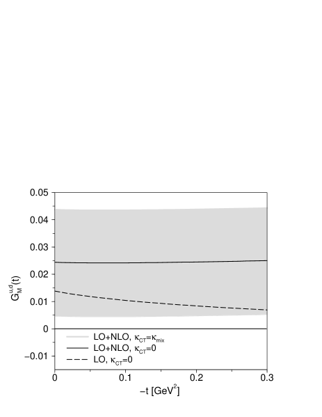
Figure 5: The form factor $G_{M}^{u,d}(t)$. The dashed line is the LO chiral prediction, the full line includes the NLO order corrections, both with $\kappa_{CT}^{u,d}(M_{\rho})=0$. The grey band is the chiral NLO representation with $\kappa_{CT}^{u,d}(M_{\rho})=-0.020\ldots+0.020$.

For the magnetic radius term, the two leading chiral contributions are unambiguously given in terms of loop effects. Evaluating Eq. (21) numerically, we find the chiral prediction at NLO to result in

$$\bigl{(}\rho_{M}^{u,d}\bigr{)}_{\chi}=\bigl{(}0.05-0.04\bigr{)}\,{\rm GeV}^{-2}=0.01\,{\rm GeV}^{-2}~{}.$$ (37)

Fig. 5 shows the purely chiral NLO representation of $G_{M}^{u,d}(t)$ in the range $0\leq-t\leq 0.3\,$GeV², together with the range of counterterm values as estimated from Eq. (31), shown as a grey band. For comparison, the LO and NLO representations are also shown for $\kappa_{CT}^{u,d}(M_{\rho})=0$. Although the uncertainty is sizeable, $G_{M}^{u,d}(t)$ is predicted to be positive and smaller than 0.05 in this range. Due to the substantial cancellation between chiral LO and NLO contributions to the magnetic radius, the $t$-dependence is very weak. Also, the curvature induced by chiral loop effects is minimal.

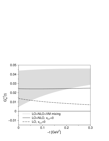
Figure 6: The form factor $G_{M}^{u,d}(t)$, notation as in Fig. 5. The grey band now includes the full $t$-dependence of the mixing amplitude. For details, see main text.

Even if the large cancellation between the LO and NLO terms for the magnetic radius is considered accidental, the (formally next-to-next-to-leading) vector meson contribution in Eq. (33) is seen to be at least of the same order of magnitude, potentially larger than both. The vector meson mixing contributions lead to a sign change in the radius as compared to the chiral prediction. Together with a positive magnetic moment, this means the form factors increase in absolute magnitude for non-vanishing virtuality in electron scattering experiments, $t<0$. This is shown in Fig. 6, where, in comparison to Fig. 5, we have replaced the low-energy constant contribution $\kappa^{u,d}_{CT}(M_{\rho})=\kappa^{u,d}_{mix}$ by the full $t$-dependence of the mixing amplitude, Eq. (28). As the complete mixing amplitude contains no more parameters than the constant at $t=0$, the uncertainty band can even get narrower: the upper boundary of the band (given by the vector meson parameters from Ref. Mergell et al. (1996)) changes very little and stays below $0.05$, while the lower boundary (given essentially by the parameters from Ref. Belushkin et al. ) rises with $-t$.

We want to emphasize that this combined chiral plus vector meson mixing representation as shown in Fig. 6 goes beyond strict effective field theory. We believe however that the additional $t$-dependence of the mixing contributions provides a good estimate of the most important higher-order terms that go beyond our chiral calculation, for the following reasons: the strongest $t$-dependence from pion loops has to correspond to cuts in the low-energy region, and among these, two-pion cuts are certainly the most prominent (see e.g. Ref. Bernard et al. (1996) on three-pion cut contributions to nucleon form factors); but we have already calculated the two-pion cuts up to NLO, and we do not expect higher-order corrections to these to be unreasonably large (witness Ref. Kaiser (2003) for two-loop corrections to the two-pion continuum). We therefore find it reasonable to expect low-energy constants (corresponding to resonance physics) to dominate the missing pieces beyond the NLO chiral representation. We have argued earlier that we expect resonance contributions beyond $\rho$–$\omega$ mixing to be minor corrections, and consider their possible impact well-covered by the uncertainty bands in Figs. 5, 6. Note finally that such a combined approach was shown to work rather well for the isospin conserving form factors in Refs. Kubis and Meißner (2001a); Kubis and Meißner (2001b).

We now turn to the electric form factor $G_{E}^{u,d}(t)$. It can only be predicted unambiguously to leading order in ChPT, where one has $G_{E}^{u,d}(t)=F_{1}^{u,d}(t)$.

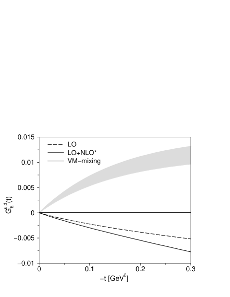
Figure 7: Contributions to the form factor $G_{E}^{u,d}(t)$. The full line is the LO chiral prediction, the dashed line contains partial NLO order corrections as discussed in the main text. The grey band is the vector meson mixing contribution.

This is shown as the dashed line in Fig. 7. A partial higher-order correction is given by the chiral contributions to $t/4m_{N}^{2}\times F_{2}^{u,d}(t)$, see Eq. (2), which is added to the leading-order expression for the full line in Fig. 7 and can be seen there to be also numerically subleading.

The leading chiral prediction for the electric radius term is, from Eq. (19) and Appendix A.1,

$$\bigl{(}\rho_{E}^{u,d}\bigr{)}_{\chi}=\frac{5\pi\,C}{6M_{\pi}m_{N}}+{\cal O}\bigl{(}M_{\pi}^{0}\Delta m\bigr{)}~{}.$$ (38)

Numerically, this amounts to

$$\bigl{(}\rho_{E}^{u,d}\bigr{)}_{\chi}=0.03\,{\rm GeV}^{-2}~{},$$ (39)

which demonstrates that the vector meson contribution, see Eq. (32), is numerically dominant, albeit formally subleading. It again leads to a sign change compared to the leading chiral prediction. This can also be seen from Fig. 7, where the full $\rho$–$\omega$ mixing amplitude is depicted as a grey band, corresponding to the range of vector meson coupling constants yielding the electric radius range in Eq. (32). Compared to $G_{M}^{u,d}(t)$, the band is better constrained as the particularly controversial coupling $\kappa^{\omega}$ plays no major role in the electric form factor.

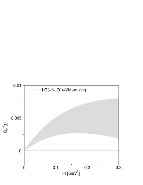
Figure 8: The complete form factor $G_{E}^{u,d}(t)$. The band combines uncertainties in the vector meson mixing amplitude as well as from higher-order chiral corrections. For details see main text.

Chiral and vector meson contributions are combined in Fig. 8, where we have taken the partial NLO chiral contributions described above as an uncertainty for higher-order loop corrections. Errors from both sources were added linearly. We consider this band a conservative estimate. Due to the bigger mixing amplitude, the total form factor is positive, but remains small ($<0.01$) and therefore well-constrained in the whole momentum transfer range considered.

Table 3: Comparison of selected experimental measurements of strange form factors to the results of this work. The column “electric/magnetic” shows the linear combination of strange electric and magnetic form factors as well as the momentum transfer in the respective kinematics, the column “$G^{s}$” the corresponding result. The column “$G^{u,d}$” gives the range of the isospin breaking form factor contributions for the same linear combination, in the same kinematics, as predicted in this work.

experiment	electric/magnetic	$G^{s}$	$G^{u,d}$
SAMPLE Spayde et al. (2004)	$G_{M}\bigl{(}-0.1\,{\rm GeV}^{2}\bigr{)}$	$0.37\pm 0.20\pm 0.26\pm 0.07$	$0.02\ldots 0.05$
A4 Maas et al. (2005)	$\bigl{[}G_{E}+0.106\,G_{M}\bigr{]}\bigl{(}-0.108\,{\rm GeV}^{2}\bigr{)}$	$0.071\pm 0.036$	$0.004\ldots 0.010$
HAPPEX Aniol et al. (2005)	$\bigl{[}G_{E}+0.080\,G_{M}\bigr{]}\bigl{(}-0.099\,{\rm GeV}^{2}\bigr{)}$	$0.030\pm 0.025\pm 0.006\pm 0.012$	$0.004\ldots 0.009$

In order to put these numbers into perspective concerning the strangeness form factor measurements, we want to compare them to some experimental results on the latter. Ref. Young et al. (2006) is a recent attempt to combine all available world data on parity violating electron scattering and perform a best fit for the leading strangeness moments. The fit including only leading-order moments (e.g. no strange magnetic radius) yields

$$\begin{split}\kappa^{s}&=0.12\pm 0.55\pm 0.07~{},\\ \rho_{E}^{s}&=\bigl{(}-0.06\pm 0.41\mp 0.00\bigr{)}\,{\rm GeV}^{-2}~{},\end{split}$$ (40)

while a fit allowing for next-to-leading-order moments results in $\rho_{M}^{s}=(0.7\pm 6.8)\,$GeV^-2, i.e. the data are not sufficiently accurate yet to pin down the magnetic radius to reasonable accuracy. So while the central values of Eq. (40) are already of comparable magnitude to $\kappa^{u,d}$, ${\rho_{E}^{u,d}}$, the isospin violating moments are still, by a factor of 6–10, smaller than the combined uncertainties on the strangeness moments.

In Table 3, we also compare to a few selected individual experimental numbers on strangeness form factors Spayde et al. (2004); Aniol et al. (2005); Maas et al. (2005). We contrast those results with bands for the isospin violating form factors in the same kinematics, i.e. for the same combination of electric and magnetic, and the same momentum transfer $t$. The error band corresponds to a worst-case combination of the bands discussed in connection with Figs. 6, 8. The conclusion is similar here: the uncertainty from isospin breaking is still smaller than the overall experimental error, but is relevant as measurements become more and more precise.

V Summary and conclusions

In this paper, we have re-investigated the isospin breaking vector form factors of the nucleon that are increasingly becoming a necessary ingredient to the precise extractions of the strange vector form factors. Our findings can be summarized as follows:

1. We calculate the isospin breaking electric and magnetic form factors $G_{E/M}^{u,d}(t)$ to leading and next-to-leading order in two-flavor chiral perturbation theory, correcting some errors in Ref. Lewis and Mobed (1999a). Up to this order of accuracy, all loop effects are due to the proton-neutron mass difference. Only one combination of unknown low-energy constants enters the chiral representation of these form factors, namely a contribution to the isospin breaking magnetic moment. Leading and next-to-leading-order contributions to the magnetic radius are seen to cancel to a large extent, leading to a very weak momentum dependence.

2. In order to estimate the missing counterterms, we employ the method of resonance saturation. We provide analytic expressions for the isospin breaking magnetic moment as well as for (formally subleading) electric and magnetic radii in terms of various vector meson coupling constants and the $\rho$–$\omega$ mixing angle. While most of these phenomenological parameters are known to apt precision, by far the most uncertain coupling is the $\omega$–nucleon tensor coupling, which dominates the rather broad error band in our prediction for the isospin breaking magnetic form factor.

3. For the electric and magnetic radii where counterterms only come in at subleading orders, we find that the combination of the relatively small nucleon mass difference, which is responsible for the chiral loop contributions, and the strong vector-meson–nucleon couplings, which numerically enhance the effect of low-energy constants, tends to upset the hierarchy suggested by chiral power counting. The vector meson mixing contributions lead to sign changes in the radii compared to the purely chiral predictions.

4. We combine chiral loop contributions and the full vector meson mixing amplitudes in a phenomenological approach, adding the various uncertainties to produce conservative error bands. We find that $G_{E/M}^{u,d}(t)$ are both positive in the momentum transfer range $0\leq-t\leq 0.3\,$GeV², with approximate upper limits $G_{M}^{u,d}(t)<0.05$, $G_{E}^{u,d}(t)<0.01$.

In order to sharpen our findings and make the prediction for the isospin breaking vector form factors even more stringent, the predominant task would be to improve on our knowledge of the $\omega$–nucleon tensor coupling, if feasible. Higher-order chiral calculations would be extremely tedious as they would involve two-loop diagrams with pions and photons, and are unlikely to be of high numerical relevance compared to the resonance physics considered in this article.

Appendix A Chiral background

A.1 Loop functions

Here we spell out the explicit forms of the loop functions used in Section III.3:

$$\begin{split}\bar{\gamma}_{0}(t)&=\frac{1}{16\pi}\biggl{(}\frac{2M_{\pi}}{\sqrt{-t}}\arctan\frac{\sqrt{-t}}{2M_{\pi}}-1\biggr{)}~{},\\ \bar{\gamma}_{3}(t)&=\frac{1}{16\pi}\biggl{(}\frac{4M_{\pi}^{2}-t}{4M_{\pi}\sqrt{-t}}\arctan\frac{\sqrt{-t}}{2M_{\pi}}-\frac{1}{2}\biggr{)}~{},~{}~{}\\ \xi(t)&=-\frac{1}{16\pi^{2}}\biggl{(}\sigma\log\frac{\sigma+1}{\sigma-1}-2\biggr{)}~{},\end{split}$$ (41)

where $\sigma=\sqrt{1-{4M_{\pi}^{2}}/{t}}$. $\bar{\gamma}_{0/3}(t)$ are linked to the loop functions $\gamma_{0/3}(t)$ used in Ref. Bernard et al. (1995) via

$$\bar{\gamma}_{0}(t)=M_{\pi}\bigl{(}\gamma_{0}(t)-\gamma_{0}(0)\bigr{)}~{},~{}~{}\bar{\gamma}_{3}(t)=M_{\pi}^{-1}\bigl{(}\gamma_{3}(t)-\gamma_{3}(0)\bigr{)}~{}.$$

The leading $t$-dependence of these functions is given by

$$\begin{split}\bar{\gamma}_{0}(t)&=\frac{t}{192\pi M_{\pi}^{2}}+{\cal O}(t^{2})~{},\\ \bar{\gamma}_{3}(t)&=-\frac{t}{192\pi M_{\pi}^{2}}+{\cal O}(t^{2}),\\ \xi(t)&=\frac{t}{96\pi^{2}M_{\pi}^{2}}+{\cal O}(t^{2})~{}.\end{split}$$ (42)

We note that the functions in Eq. (41) are the heavy-baryon loop functions that were reproduced from the infrared regularized loops by strict expansion in chiral powers. As we are only interested in the form factors in the space-like region, we disregard the complications ensuing from the anomalous threshold of the triangle diagram. We want to emphasize, though, that these representations do not reproduce the correct threshold behavior of the spectral functions.

A.2 Separate diagrams

For completeness, we show here the various contributions to ${F_{1/2}^{\!\not\,v}}(0)$, ${F_{1/2}^{\!\not\,s}}(0)$ from the diagrams displayed in Fig. 1. Of course ${F_{1}^{\!\not\,v}}(0)={F_{1}^{\!\not\,s}}(0)=0$ in the sum of all diagrams is a necessary requirement. The prefactor $C$ is as defined in Eq. (14).

$${F_{1}^{\!\not\,v}}(0)\bigl{[}\text{(a)}\bigr{]} =-2{F_{1}^{\!\not\,v}}\bigl{[}\text{(b)}\bigr{]}=-2{F_{1}^{\!\not\,v}}\bigl{[}\text{(c)}\bigr{]}=\frac{6\pi M_{\pi}}{m_{N}}\,C~{},$$

$${F_{1}^{\!\not\,s}}\bigl{[}\text{(b)}\bigr{]} =-{F_{1}^{\!\not\,s}}\bigl{[}\text{(c)}\bigr{]}=\frac{3\pi M_{\pi}}{m_{N}}\,C~{},$$ (43)

$${F_{2}^{\!\not\,v}}(0)\bigl{[}\text{(a)}\bigr{]} =4\biggl{[}1+2\log\frac{M_{\pi}}{\lambda}-\frac{4\pi M_{\pi}}{m_{N}}\biggr{]}\,C~{},$$

$${F_{2}^{\!\not\,v}}\bigl{[}\text{(b)}\bigr{]} =-{F_{2}^{\!\not\,s}}\bigl{[}\text{(b)}\bigr{]}=\frac{4\pi M_{\pi}}{m_{N}}\,C~{},$$

$${F_{2}^{\!\not\,v}}\bigl{[}\text{(d)}\bigr{]} =-\frac{1}{3}{F_{2}^{\!\not\,v}}\bigl{[}\text{(e)}\bigr{]}=\frac{\pi(\kappa_{p}-\kappa_{n})M_{\pi}}{m_{N}}\,C~{},$$

$${F_{2}^{\!\not\,s}}\bigl{[}\text{(d)}\bigr{]} =\frac{1}{3}{F_{2}^{\!\not\,s}}\bigl{[}\text{(e)}\bigr{]}=-\frac{\pi(\kappa_{p}+\kappa_{n})M_{\pi}}{m_{N}}\,C~{}.$$ (44)

Appendix B Vector meson coupling constants

In this appendix, we briefly spell out how to relate the vector-meson–nucleon coupling constants used in this paper to those in Refs. Kaiser (2003); Mergell et al. (1996); Hammer and Meißner (2004); Belushkin et al. .

In Ref. Kaiser (2003), the strength of the $\rho$ contributions to the isovector spectral functions of the Sachs form factors is parameterized in terms of two coupling constants $b_{E,M}$ that are given in terms of $g_{\rho}$, $\kappa_{\rho}$ according to

$$b_{E}=\frac{g_{\rho}F_{\rho}}{2M_{\rho}}\biggl{(}1+\frac{\kappa_{\rho}M_{\rho}^{2}}{4m_{N}^{2}}\biggr{)}~{},\quad b_{M}=\frac{g_{\rho}F_{\rho}}{2M_{\rho}}\bigl{(}1+\kappa_{\rho}\bigr{)}~{}.$$ (45)

In Ref. Kaiser (2003), the numerical values $b_{E}=1.0$, $b_{M}=3.6$ were extracted. Using the updated empirical isovector spectral function from Ref. Belushkin et al. (2006), we find the slightly shifted numbers $b_{E}=1.1$, $b_{M}=3.7$, while fitting the phenomenological $\rho$ contribution with just the one-loop two-pion continuum leads to $b_{E}=1.2$, $b_{M}=4.2$. These numbers, together with Eq. (45), feed into Table 1.

The $\omega$ coupling constants are given as pole residues $a_{1,2}^{\omega}$ in the isoscalar spectral functions of Dirac and Pauli form factors in Refs. Mergell et al. (1996); Hammer and Meißner (2004); Belushkin et al. . The coupling constants $g_{\omega}$, $\kappa_{\omega}$ can be calculated from these as

$$g_{\omega}=\frac{2a_{1}^{\omega}}{F_{\omega}M_{\omega}}~{},\quad\kappa_{\omega}=\frac{a_{2}^{\omega}}{a_{1}^{\omega}}~{}.$$ (46)

The pole residues from Ref. Belushkin et al. used for Table 2 are $a_{1}^{\omega}=0.752$ GeV², $a_{2}^{\omega}=0.425$ GeV².

References

- Spayde et al. (2004) D. T. Spayde et al. (SAMPLE), Phys. Lett. B583, 79 (2004), eprint nucl-ex/0312016.
- Maas et al. (2004) F. E. Maas et al. (A4), Phys. Rev. Lett. 93, 022002 (2004), eprint nucl-ex/0401019.
- Maas et al. (2005) F. E. Maas et al., Phys. Rev. Lett. 94, 152001 (2005), eprint nucl-ex/0412030.
- Aniol et al. (2006) K. A. Aniol et al. (HAPPEX), Phys. Rev. Lett. 96, 022003 (2006), eprint nucl-ex/0506010.
- Aniol et al. (2005) K. A. Aniol et al. (HAPPEX) (2005), eprint nucl-ex/0506011.
- Armstrong et al. (2005) D. S. Armstrong et al. (G0), Phys. Rev. Lett. 95, 092001 (2005), eprint nucl-ex/0506021.
- Dong et al. (1998) S. J. Dong, K. F. Liu, and A. G. Williams, Phys. Rev. D58, 074504 (1998), eprint hep-ph/9712483.
- Mathur and Dong (2001) N. Mathur and S.-J. Dong (Kentucky Field Theory), Nucl. Phys. Proc. Suppl. 94, 311 (2001), eprint hep-lat/0011015.
- Lewis et al. (2003) R. Lewis, W. Wilcox, and R. M. Woloshyn, Phys. Rev. D67, 013003 (2003), eprint hep-ph/0210064.
- Leinweber et al. (2005a) D. B. Leinweber et al., Phys. Rev. Lett. 94, 212001 (2005a), eprint hep-lat/0406002.
- Leinweber et al. (2005b) D. B. Leinweber et al., Eur. Phys. J. A24S2, 79 (2005b), eprint hep-lat/0502004.
- Leinweber et al. (2006) D. B. Leinweber et al. (2006), eprint hep-lat/0601025.
- Musolf and Ito (1997) M. J. Musolf and H. Ito, Phys. Rev. C55, 3066 (1997), eprint nucl-th/9607021.
- Hemmert et al. (1998) T. R. Hemmert, U.-G. Meißner, and S. Steininger, Phys. Lett. B437, 184 (1998), eprint hep-ph/9806226.
- Hemmert et al. (1999) T. R. Hemmert, B. Kubis, and U.-G. Meißner, Phys. Rev. C60, 045501 (1999), eprint nucl-th/9904076.
- Hammer et al. (2003) H. W. Hammer, S. J. Puglia, M. J. Ramsey-Musolf, and S.-L. Zhu, Phys. Lett. B562, 208 (2003), eprint hep-ph/0206301.
- Kubis (2005) B. Kubis, Eur. Phys. J. A24S2, 97 (2005), eprint nucl-th/0504004.
- Silva et al. (2004) A. Silva, H.-C. Kim, and K. Goeke, Eur. Phys. J. A22, 481 (2004), eprint hep-ph/0210189.
- Silva et al. (2005) A. Silva, H.-C. Kim, D. Urbano, and K. Goeke (2005), eprint hep-ph/0601239.
- Jido and Weise (2005) D. Jido and W. Weise, Phys. Rev. C72, 045203 (2005), eprint nucl-th/0504012.
- Carvalho et al. (2005) F. Carvalho, F. S. Navarra, and M. Nielsen, Phys. Rev. C72, 068202 (2005), eprint nucl-th/0509042.
- Chen et al. (2004) X.-S. Chen, R. G. E. Timmermans, W.-M. Sun, H.-S. Zong, and F. Wang, Phys. Rev. C70, 015201 (2004).
- Bijker (2005) R. Bijker (2005), eprint nucl-th/0511060.
- An et al. (2006) C. S. An, D. O. Riska, and B. S. Zou, Phys. Rev. C73, 035207 (2006), eprint hep-ph/0511223.
- Riska and Zou (2005) D. O. Riska and B. S. Zou (2005), eprint nucl-th/0512102.
- Ramsey-Musolf (2005) M. J. Ramsey-Musolf, Eur. Phys. J. A24S2, 197 (2005), eprint nucl-th/0501023.
- Dmitrasinovic and Pollock (1995) V. Dmitrasinovic and S. J. Pollock, Phys. Rev. C52, 1061 (1995), eprint hep-ph/9504414.
- Miller (1998) G. A. Miller, Phys. Rev. C57, 1492 (1998), eprint nucl-th/9711036.
- Lewis and Mobed (1999a) R. Lewis and N. Mobed, Phys. Rev. D59, 073002 (1999a), eprint hep-ph/9810254.
- Ma (1997) B.-Q. Ma, Phys. Lett. B408, 387 (1997), eprint hep-ph/9707226.
- Thomas et al. (2005) A. W. Thomas, R. D. Young, and D. B. Leinweber (2005), eprint nucl-th/0509082.
- Gardner et al. (1996) S. Gardner, C. J. Horowitz, and J. Piekarewicz, Phys. Rev. C53, 1143 (1996), eprint nucl-th/9508035.
- Becher and Leutwyler (1999) T. Becher and H. Leutwyler, Eur. Phys. J. C9, 643 (1999), eprint hep-ph/9901384.
- Lewis and Mobed (1999b) R. Lewis and N. Mobed, PiN Newslett. 15, 144 (1999b), eprint hep-ph/9910455.
- Jenkins and Manohar (1991) E. Jenkins and A. V. Manohar, Phys. Lett. B255, 558 (1991).
- Bernard et al. (1995) V. Bernard, N. Kaiser, and U.-G. Meißner, Int. J. Mod. Phys. E4, 193 (1995), eprint hep-ph/9501384.
- Ecker et al. (1989a) G. Ecker, J. Gasser, A. Pich, and E. de Rafael, Nucl. Phys. B321, 311 (1989a).
- Fettes et al. (2000) N. Fettes, U.-G. Meißner, M. Mojžiš, and S. Steininger, Ann. Phys. 283, 273 (2000), eprint hep-ph/0001308.
- Müller and Meißner (1999) G. Müller and U.-G. Meißner, Nucl. Phys. B556, 265 (1999), eprint hep-ph/9903375.
- Bég and Zepeda (1972) M. A. B. Bég and A. Zepeda, Phys. Rev. D6, 2912 (1972).
- Ecker et al. (1989b) G. Ecker, J. Gasser, H. Leutwyler, A. Pich, and E. de Rafael, Phys. Lett. B223, 425 (1989b).
- Donoghue et al. (1989) J. F. Donoghue, C. Ramirez, and G. Valencia, Phys. Rev. D39, 1947 (1989).
- Bernard et al. (1997) V. Bernard, N. Kaiser, and U.-G. Meißner, Nucl. Phys. A615, 483 (1997), eprint hep-ph/9611253.
- Kubis and Meißner (2001a) B. Kubis and U.-G. Meißner, Nucl. Phys. A679, 698 (2001a), eprint hep-ph/0007056.
- Höhler et al. (1976) G. Höhler et al., Nucl. Phys. B114, 505 (1976).
- Mergell et al. (1996) P. Mergell, U.-G. Meißner, and D. Drechsel, Nucl. Phys. A596, 367 (1996), eprint hep-ph/9506375.
- Hammer and Meißner (2004) H.-W. Hammer and U.-G. Meißner, Eur. Phys. J. A20, 469 (2004), eprint hep-ph/0312081.
- Urech (1995) R. Urech, Phys. Lett. B355, 308 (1995), eprint hep-ph/9504238.
- Gasser and Leutwyler (1982) J. Gasser and H. Leutwyler, Phys. Rept. 87, 77 (1982).
- Kucurkarslan and Meißner (2006) A. Kucurkarslan and U.-G. Meißner (2006), eprint hep-ph/0603061.
- Borasoy and Meißner (1996) B. Borasoy and U.-G. Meißner, Int. J. Mod. Phys. A11, 5183 (1996), eprint hep-ph/9511320.
- Bijnens and Gosdzinsky (1996) J. Bijnens and P. Gosdzinsky, Phys. Lett. B388, 203 (1996), eprint hep-ph/9607462.
- Benayoun and O’Connell (2001) M. Benayoun and H. B. O’Connell, Eur. Phys. J. C22, 503 (2001), eprint nucl-th/0107047.
- Eidelman et al. (2004) S. Eidelman et al. (Particle Data Group), Phys. Lett. B592, 1 (2004).
- Machleidt et al. (1987) R. Machleidt, K. Holinde, and C. Elster, Phys. Rept. 149, 1 (1987).
- Stoks et al. (1994) V. G. J. Stoks, R. A. M. Klomp, C. P. F. Terheggen, and J. J. de Swart, Phys. Rev. C49, 2950 (1994), eprint nucl-th/9406039.
- Davidson et al. (1991) R. M. Davidson, N. C. Mukhopadhyay, and R. S. Wittman, Phys. Rev. D43, 71 (1991).
- Pasquini et al. (2006) B. Pasquini, D. Drechsel, and L. Tiator, Eur. Phys. J. A27, 231 (2006), eprint nucl-th/0603006.
- Bernard et al. (1996) V. Bernard, N. Kaiser, and U.-G. Meißner, Nucl. Phys. A611, 429 (1996), eprint hep-ph/9607428.
- Mergell (1995) P. Mergell, Master’s thesis, Johann-Gutenberg-Universität Mainz, Institut für Kernphysik (1995).
- Belushkin et al. (2006) M. A. Belushkin, H.-W. Hammer, and U.-G. Meißner, Phys. Lett. B633, 507 (2006), eprint hep-ph/0510382.
- Kaiser (2003) N. Kaiser, Phys. Rev. C68, 025202 (2003), eprint nucl-th/0302072.
- (63) M. A. Belushkin, H.-W. Hammer, and U.-G. Meißner, in preparation.
- Kubis and Meißner (2001b) B. Kubis and U.-G. Meißner, Eur. Phys. J. C18, 747 (2001b), eprint hep-ph/0010283.
- Young et al. (2006) R. D. Young, J. Roche, R. D. Carlini, and A. W. Thomas (2006), eprint nucl-ex/0604010.