Dissipative hydrodynamics in 2+1 dimension

Abstract

In 2+1 dimension, we have simulated the hydrodynamic evolution of QGP fluid with dissipation due to shear viscosity. Comparison of evolution of ideal and viscous fluid, both initialised under the same conditions e.g. same equilibration time, energy density and velocity profile, reveal that the dissipative fluid evolves slowly, cooling at a slower rate. Cooling get still slower for higher viscosity. The fluid velocities on the otherhand evolve faster in a dissipative fluid than in an ideal fluid. The transverse expansion is also enhanced in dissipative evolution. For the same decoupling temperature, freeze-out surface for a dissipative fluid is more extended than an ideal fluid. Dissipation produces entropy as a result of which particle production is increased. Particle production is increased due to (i) extension of the freeze-out surface and (ii) change of the equilibrium distribution function to a non-equilibrium one, the last effect being prominent at large transverse momentum. Compared to ideal fluid, transverse momentum distribution of pion production is considerably enhanced. Enhancement is more at high $p_{T}$ than at low $p_{T}$. Pion production also increases with viscosity, larger the viscosity, more is the pion production. Dissipation also modifies the elliptic flow. Elliptic flow is reduced in viscous dynamics. Also, contrary to ideal dynamics where elliptic flow continues to increase with transverse momentum, in viscous dynamics, elliptic flow tends to saturate at large transverse momentum. The analysis suggest that initial conditions of the hot, dense matter produced in Au+Au collisions at RHIC, as extracted from ideal fluid analysis can be changed significantly if the QGP fluid is viscous.

I Introduction

Lattice QCD predicts that under certain conditions (sufficiently high energy density and temperature), ordinary hadronic matter (where quarks and gluons are confined), can undergo a phase transition to a deconfined matter, commonly known as Quark Gluon Plasma (QGP). Nuclear physicists are trying to produce and detect this new phase of matter at RHIC, BNL. Recent Au+Au collisions at RHIC, indicate that dense, color opaque medium of deconfined matter is created in very central collisions BRAHMSwhitepaper ; PHOBOSwhitepaper ; PHENIXwhitepaper ; STARwhitepaper . It is now also understood that the quarks and gluons strongly interact, giving rise to the notion of sQGP (strongly interacting QGP). The experimental data are successfully analysed in a ideal fluid dynamic model QGP3 . Hydrodynamic evolution of ideal QGP, thermalised at $\tau_{i}$=0.6 fm, with central entropy density of 110 $fm^{-3}$, or energy density of 35 $GeV/fm^{3}$ can explain a large volume of RHIC data, the $p_{T}$ spectra of identified particles, the elliptic flow etc QGP3 . However, experimental data do show deviation from ideal behavior. The ideal fluid description works well in almost central Au+Au collisions near mid-rapidity at top RHIC energy, but gradually breaks down in more peripheral collisions, at forward rapidity, or at lower collision energies Heinz:2004ar , indicating the onset of dissipative effects. To describe such deviations from ideal fluid dynamics quantitatively, requires the numerical implementation of dissipative relativistic fluid dynamics.

Eckart Eckart and Landau and Lifshitz LL63 formulated the theory of dissipative relativistic fluid. Their theories are called first order theories and suffer from the problem of causality; the signal can travel faster than light. 1st order theories assume that the entropy 4-current contains terms upto linear order in dissipative quantities. This restriction results in parabolic equations, which leads to causality problem. The causality problem is removed in the 2nd-order theories, formulated by Israel and Stewart IS79 . In 2nd order theories, dissipative fluxes are treated as (extended) thermodynamic variables and the linear relation between entropy 4-current and dissipative quantities is extended to include quadratic terms. The entropy 4-current contains terms upto 2nd order in dissipative forces. The resulting equations are hyperbolic in nature and the causality problem is removed. Naturally 2nd order theories are more complicated. In addition to the usual energy-momentum conservations equations, relaxation equations for dissipative fluxes are required to be solved simultaneously.

Though the theories of dissipative hydrodynamics Eckart ; LL63 ; IS79 has been known for more than 30 years , significant progress towards its numerical implementation has only been made very recently Muronga:2001zk ; Teaney:2004qa ; MR04 ; CH05 ; Heinz:2005bw . Earlier attempts were restricted to simple one-dimensional Bjorken expansion vis_bj . Since the hot dense matter, produced in RHIC collisions, undergoes large transverse expansion, such models are not of much help in extracting initial conditions of the fluid from the experiment. Recently Teaney Teaney:2004qa solved the hydrodynamic equations in a 1st order dissipative theory. He used the blast wave model and calculated the corrections to thermal distribution functions considering shear viscosity only. Blast wave models lack dynamics. Freeze-out surface is parameterised and one fit the freeze-out parameters with experimental observables. Information about the initial conditions of the hot dense matter is not available in blast wave models. In MR04 ; CH05 , 2nd order theories for dissipative fluid, is solved for QGP fluid. While the models are dynamic, (energy-momentum conservation equations are solved) energy-momentum conservation equations are solved in 1+1 dimension, assuming longitudinal boost-invariance and cylindrical symmetry. Thus these models do not give any information on the most sensitive experimental observable, the elliptic flow. Recently in Heinz:2005bw explicit equations describing the space-time evolution of non-ideal relativistic fluid, undergoing boost-invariant longitudinal and arbitrary transverse expansion, are given. Equations are written for both the 1st order and 2nd order theory.

At the Variable Energy Cyclotron Centre, Kolkata, we have developed a numerical code (AZHYDRO-KOLKATA) to solve, both the 1st order and 2nd order dissipative hydrodynamics in 2+1 dimension. In the present paper we will present AZHYDRO-KOLKATA results for the 1st order dissipative hydrodynamics. Results for 2nd order dissipative hydrodynamics will be presented in a later publication. As mentioned earlier, 1st order theories are acausal, signal can travel faster than light. In one dimension, 1st order theories can be solved analytically. Analytical solutions indicate that at early time, an unphysical reheating of the fluid can occur MR04 ; Baier:2006um . Even though in the present simulation, we donot find any indication of early reheating, nevertheless, we maintain that only 2nd order results, which do not have the unphysical causality the problem are more reliable. In this paper we will be concerned mainly with the effect of viscosity on fluid evolution and its affects the particle production; $p_{T}$ distribution and elliptic flow. No attempt will be made to explain experimental data.

Paper is organised as follows: in section II, we describe briefly the hydrodynamic equations needed for 1st order dissipative hydro-dynamics. In section III, we describe the equation of state, shear viscosity coefficient and initial conditions used in the present study. With dissipation, equilibrium distribution function is changed. Correction to equilibrium distribution function due to non-equilibrium effects are described in section IV. We have studied particle (pion) production in the model. The relevant equations for pion production with the equilibrium distribution function and its correction due to non-equilibrium effects, are discussed in section V. Results of the numerical simulations are shown in section VI. Lastly, in section VII, summary and conclusions are drawn.

II 1st order dissipative fluid dynamics

Relativistic dissipative hydrodynamics and associated equations in 2+1 dimensions has been discussed in detail in ref.Heinz:2005bw . Any fluid dynamical approach starts from the conservation laws for the conserved charges and for energy-momentum. For a singly charged fluid, the conservation laws are:

$$\partial_{\mu}N^{\mu} = 0$$ (1)

$$\partial_{\mu}T^{\mu\nu} = 0.$$ (2)

It must also ensure the second law of thermodynamics

$$\partial_{\mu}S^{\mu}\geq 0,$$ (3)

where $S^{\mu}$ is the entropy current.

In the present paper we restrict ourselves to central rapidity region, where the QGP fluid is essentially baryon free. We thus neglect Eq.1. To keep the calculations simple, we consider the most important dissipative term, the shear viscosity and neglect the other dissipative terms, e.g. heat conduction, bulk viscosity. For a baryon free fluid, the heat conduction is zero. Bulk viscosity is zero for QGP (point particles). Bulk viscosity will be non-zero in the hadronic phase but presently we neglect it.

With the help of hydrodynamic 4-velocity $u^{\mu}$ (normalised as $u^{\mu}u_{\mu}=1$) and projector $\Delta^{\mu\nu}=g^{\mu\nu}-u^{\mu}u^{\nu}$, with only shear viscosity as the dissipative flux, in Landau’s frame, the energy momentum tensor, and the entropy 4-current, can be decomposed as,

$$T^{\mu\nu}=T_{\rm eq}^{\mu\nu}+\delta T^{\mu\nu}=\varepsilon\,u^{\mu}u^{\nu}-p\Delta^{\mu\nu}+\pi^{\mu\nu}$$ (4)

$$S^{\mu}=S^{\mu}_{\rm eq}+\delta S^{\mu}=s\,u^{\mu}+\Phi^{\mu}.$$ (5)

where $\varepsilon=u_{\mu}T^{\mu\nu}u_{\nu}$ is the energy density, $p$ is the local pressure. $\pi^{\mu\nu}$ is the non-ideal part of the energy-momentum tensor, the stress tensor due to shear viscosity. $s=u_{\mu}S^{\mu}$ is the entropy density and $\Phi^{\mu}$ is the entropy flux due to dissipation.

In the first order theories, the shear stress tensors are written as,

$$\pi^{\mu\nu}=2\eta\nabla^{<\mu}u^{\nu>}$$ (6)

where $\eta$ is the shear viscosity coefficient and $\nabla^{<\mu}u^{\nu>}$ is a trace-less symmetric tensor defined as,

$$\nabla^{<\mu}u^{\nu>}=\left[\frac{1}{2}\left(\Delta^{\mu\sigma}\Delta^{\nu\tau}{+}\Delta^{\nu\sigma}\Delta^{\mu\tau}\right)-\frac{1}{3}\Delta^{\mu\nu}\Delta^{\sigma\tau}\right]$$ (7)

Viscous pressure $\pi^{\mu\nu}$ is symmetric ($\pi^{\mu\nu}=\pi^{\nu\mu}$), traceless ($\pi^{\mu}_{\mu}=0$) and transverse to hydrodynamic velocity, ($u_{\mu}\pi^{\mu\nu}=0)$. The 16-component $\pi^{\mu\nu}$ has only 5 independent components. As mentioned in the beginning, we have solved the equations with the assumption of longitudinal boost-invariance. With boost-invariance the number of independent shear-stress tensors further reduces to 3.

Heavy ion collisions are best described in terms of proper time $\tau=\sqrt{t^{2}-z^{2}}$ and rapidity $\eta_{s}=\frac{1}{2}\ln\frac{t+z}{t-z}$ (we use the subscript $s$ to distinguish spatial rapidity from the viscous coefficient $\eta$). In $(\tau,x,y,\eta_{s})$ coordinates, with longitudinal boost-invariance, the hydrodynamic 4-velocity can be written as,

$$u^{\mu}= (u^{\tau},u^{x},u^{y},u^{\eta_{s}})$$

$$= (\gamma_{\perp},\gamma_{\perp}v_{x},\gamma_{\perp}v_{y},0),$$ (8)

with $\gamma_{\perp}=1/\sqrt{1-v_{x}^{2}-v_{y}^{2}}$. Explicit equations for energy-momentum conservation, in $(\tau,x,y,\eta_{s})$ coordinate system has been developed in ref.Heinz:2005bw . Here we rewrite the results in a form suitable for numerical algorithm. The energy-momentum conservation equations are,

$$\partial_{\tau}\Bigl{(}\tilde{T}^{\tau\tau}\Bigr{)}+\partial_{x}\Bigl{(}\tilde{T}^{\tau\tau}\overline{v}_{x}\Bigr{)}+\partial_{y}\Bigl{(}\tilde{T}^{\tau\tau}\overline{v}_{y}\Bigr{)}=-\,(p+\tau^{2}\pi^{\eta\eta}),$$ (9)

$$\partial_{\tau}\Bigl{(}\tilde{T}^{\tau x}\Bigr{)}+\partial_{x}\Bigl{(}\tilde{T}^{\tau x}v_{x}\Bigr{)}+\partial_{y}\Bigl{(}\tilde{T}^{\tau x}v_{y}\Bigr{)}=-\partial_{x}(\tilde{p}+\tilde{\pi}^{xx}-\tilde{\pi}^{\tau x}v_{x})-\partial_{y}(\tilde{\pi}^{xy}-\tilde{\pi}^{\tau x}v_{y}),$$ (10)

$$\partial_{\tau}\Bigl{(}\tilde{T}^{\tau y}\Bigr{)}+\partial_{x}\Bigl{(}\tilde{T}^{\tau y}v_{x}\Bigr{)}+\partial_{y}\Bigl{(}\tilde{T}^{\tau y}v_{y}\Bigr{)}=-\partial_{x}(\tilde{\pi}^{xy}-\tilde{\pi}^{\tau y}v_{x})-\partial_{y}(\tilde{p}+\tilde{\pi}^{yy}-\tilde{\pi}^{\tau y}v_{y}),$$ (11)

where $\overline{v}_{x}=T^{\tau x}/T^{\tau\tau}$ and $\overline{v}_{y}=T^{\tau y}/T^{\tau\tau}$, and we have used the notation ”tilde” to represent quantities multiplied by the factor $\tau$, $\tilde{p}=\tau p$ and similarly $\tilde{T}^{ij}=\tau T^{ij}$. We note that unlike in ideal fluid, in viscous fluid dynamics conservation equations contain additional pressure gradients containing the dissipative fluxes. Both $T^{\tau x}$ and $T^{\tau y}$ components of energy-momentum tensors now evolve under the influence of additional pressure gradients.

In 1st order theory, the shear stress tensor components required in the preceding equations are,

$$\pi^{\tau x}=2\eta[-\frac{1}{2}\partial_{x}\gamma_{\perp}+\frac{1}{2}\partial_{\tau}(\gamma_{\perp}v_{x})-\frac{1}{2}D(\gamma_{\perp}^{2}v_{x})+\frac{\theta}{3}\,\gamma_{\perp}^{2}v_{x}],$$ (12)

$$\pi^{\tau x}=2\eta[-\frac{1}{2}\partial_{y}\gamma_{\perp}+\frac{1}{2}\partial_{\tau}(\gamma_{\perp}v_{y})-\frac{1}{2}D(\gamma_{\perp}^{2}v_{y})+\frac{\theta}{3}\,\gamma_{\perp}^{2}v_{y}],$$ (13)

$$\pi^{\tau\tau}=2\eta[\frac{\theta}{3}(\gamma_{\perp}^{2}-1)+\partial_{\tau}\gamma_{\perp}-\frac{1}{2}D(\gamma_{\perp}^{2})],$$ (14)

$$\pi^{\eta\eta}=2\eta[\frac{1}{\tau^{2}}\left(\frac{\theta}{3}-\frac{\gamma_{\perp}}{\tau}\right)],$$ (15)

$$\pi^{xx}=2\eta[-\partial_{x}(\gamma_{\perp}v_{x})-\frac{1}{2}D(\gamma_{\perp}^{2})+\frac{\theta}{3}(1+\gamma_{\perp}^{2}v_{x}^{2})],$$ (16)

$$\pi^{yy}=2\eta[-\partial_{x}(\gamma_{\perp}v_{y})-\frac{1}{2}D(\gamma_{\perp}^{2})+\frac{\theta}{3}(1+\gamma_{\perp}^{2}v_{y}^{2})]$$ (17)

where $D=u^{\mu}\partial_{\mu}$ is the convective time derivative,

$$D=\gamma_{\perp}(\partial_{\tau}+v_{x}\partial_{x}+v_{y}\partial_{y}),$$ (18)

and $\theta$ is the local expansion rate, given by,

$$\theta=\frac{\gamma_{\perp}}{\tau}+\partial_{\tau}\gamma_{\perp}+\partial_{x}(v_{x}\gamma_{\perp})+\partial_{y}(v_{y}\gamma_{\perp})$$ (19)

Given an equation of state, if energy density ($\varepsilon$) and fluid velocity ($v_{x}$ and $v_{y}$) distributions, at any time $\tau_{i}$ are known, Eqs.9,10 and 11 can be integrated to obtain $\varepsilon$,$v_{x}$ and $v_{y}$ at the next time step $\tau_{i+1}$. While for ideal hydrodynamics, this procedure works perfectly, viscous hydrodynamics poses a problem that shear stress-tensor components contains time derivatives, $\partial_{\tau}\gamma_{\perp}$, $\partial_{\tau}u^{x}$, $\partial_{\tau}u^{x}$ etc. Thus at time step $\tau_{i}$ one needs the still unknown time derivatives. In 1st order theories, this problem is circumvented by calculating the time derivatives from the ideal equation of motion,

$$Du^{\mu} = \frac{\nabla^{\mu}p}{\varepsilon+p},$$ (20)

$$D\varepsilon = -(\varepsilon+p)\nabla_{\mu}u^{\mu}.$$ (21)

With the help of these two equations all the time derivatives can be expressed entirely in terms of spatial gradients. 1st order theories are restricted to contain terms at most linear in dissipative quantities. Neglect of viscous terms can contribute only in 2nd order corrections, which is neglected in 1st order theories.

III Equation of state, viscosity coefficient and initial conditions

III.1 Equation of state

One of the most important inputs of a hydrodynamic model is the equation of state. Through this input, the macroscopic hydrodynamic models make contact with the microscopic world. In the present calculation we have used the equation of state, EOS-Q, developed in ref.QGP3 . It is a two-phase equation of state. The hadronic phase of EOS-Q is modeled as a non-interacting gas of hadronic resonance. As the temperature is increased, larger and larger fraction of available energy goes into production of heavier and heavier resonances. This results into a soft equation of state, with small speed of sound, $c^{2}_{s}\approx 0.15$. With increasing temperature, the available volume is filled up with resonances and the hadronic states starts to overlap, and microscopic degrees of freedom are changed from hadron to deconfined quarks and gluons. The QGP phase is modeled as that of a non-interacting quark (u,d and s) and gluons, confined by a bag pressure B. Corresponding equation of state, $p=\frac{1}{3}e-\frac{4}{3}B$ is stiff with a speed of sound $c_{s}^{2}=\frac{1}{3}$. The two phases are matched by Maxwell construction at the critical temperature, $T_{c}=164MeV$, adjusting the Bag pressure $B^{1/4}$=230 MeV. As discussed in QGP3 , ideal hydrodynamics explain a large volume of RHIC Au+Au data with EOS-Q.

III.2 Shear viscosity coefficient

Shear viscosity coefficient ($\eta$) of dense nuclear (QGP or resonance hadron gas) is quite uncertain. In perturbative regime, shear viscosity of a QGP is estimated Arnold:2000dr ; Baym:1990uj ,

$$\eta=86.473\frac{1}{g^{4}}\frac{T^{3}}{logg^{-1}},$$ (22)

With entropy of QGP, $s=37\frac{\pi^{2}}{15}T^{3}$ and $\alpha_{s}\approx$0.5, the ratio of viscosity over the entropy, in the perturbative regime is estimated as,

$$\left(\frac{\eta}{s}\right)_{pert}\approx 0.135,$$ (23)

However, QGP produced in nuclear collisions is non-perturbative. It is strongly interacting QGP. Recently, using the ADS/CFT correspondence Policastro:2001yc ; Policastro:2002se , shear viscosity of a strongly coupled gauze theory, N=4 SUSY YM, has been evaluated, $\eta=\frac{\pi}{8}N^{2}_{c}T^{3}$ and the entropy is given by $s=\frac{\pi^{2}}{2}N^{2}_{c}T^{3}$. Thus in the strongly coupled field theory,

$$\left(\frac{\eta}{s}\right)_{ADS/CFT}=\frac{1}{4\pi}\approx 0.08,$$ (24)

which is 2 times larger than the perturbative estimate. In the present paper, we treat the shear viscosity as a parameter of the model. To demonstrate the effect of viscosity on flow and subsequent particle production, we use both the perturbative and ADS/CFT estimate of viscosity.

1st order theories are acuasal. As mentioned earlier, unphysical effects like reheating of the fluid, early in the evolution, can occur. In one dimension energy-momentum conservation equation can be solved analytically. If initial fluid temperature is $T_{i}$ at initial time $\tau_{i}$, for constant $\eta/s$, the fluid temperature at time $\tau$ can be obtained as Baier:2006um ,

$$T(\tau)=T_{i}\left(\frac{\tau_{i}}{\tau}\right)^{1/3}\left[1+\frac{2}{3\tau_{i}T_{i}}\frac{\eta}{s}\left(1-\left(\frac{\tau_{i}}{\tau}\right)^{2/3}\right)\right]$$ (25)

For early times, $\tau<\tau_{max}$,

$$\tau_{max}=\tau_{i}\left(\frac{1}{3}+\frac{s}{\eta}\frac{\tau_{i}T_{i}}{2}\right)^{-3/2},$$ (26)

the solution shows an unphysical reheating. The unphysical reheating is minimised if $\tau_{max}$ is small or $\eta/s<<\tau_{i}T_{i}$. As will be explained below, we have used an initial time $\tau_{i}$=0.6 fm/c and initial temperature of the fluid, $T_{i}$=0.35 GeV . For both the values of viscosity, $\eta/s<<\tau_{i}T_{i}$, the unphysical reheating is minimised.

Shear viscosity can also be expressed in terms of sound attenuation length, $\Gamma_{s}$, defined as,

$$\Gamma_{s}=\frac{\frac{4\eta}{3}}{sT}$$ (27)

$\Gamma_{s}$ is equivalent to mean free path and for a valid hydrodynamic description $\Gamma_{s}/\tau<<1$, i.e. mean free path is much less than the system size. With the present choice of equilibration time and temperature, both for ADS/CFT and perurbative estimate of viscosity, at initial time, $\Gamma_{s}/\tau$ is much less than unity and hydrodynamics remains a valid description. At later time the validity condition becomes even better.

III.3 Initial conditions

As discussed earlier, ideal hydrodynamics has been very successful in explain a large volume of data in RHIC 200AGeV Au+Au collisions QGP3 . In the present demonstrative calculations, we have used the similar initial conditions as in ref.QGP3 . Details of the initial conditions can be found in QGP3 . We just mention that in ref.QGP3 , initial transverse energy is parameterised geometrically. At an impact parameter $\vec{b}$, transverse distribution of wounded nucleons $N_{WN}(x,y,\vec{b})$ and of binary NN collisions $N_{BC}(x,y,\vec{b})$ to are calculated in a Glauber model. A collision at impact parameter $\vec{b}$ is assumed to contain 25% hard scattering (proportional to number of binary collisions) and 75% soft scattering (proportional to number of wounded nucleons). Transverse energy density profile at impact parameter $\vec{b}$ is then obtained as,

$$\varepsilon(x,y,\vec{b})=\varepsilon_{0}(0.75\times N_{WN}(x,y,\vec{b})+0.25\times N_{BC}(x,y,\vec{b}))$$ (28)

The parameter $\varepsilon_{0}$ and the initial equilibration time $\tau_{i}$ are fixed to reproduce the experimental transverse momentum distribution of pions in central Au+Au collisions. STAR and PHENIX data are fitted to obtain initial equilibrium time $\tau_{i}$=0.6 fm and central entropy density of $s=110fm^{-3}$. This corresponds energy density of the fluid as 25 $GeV/fm^{3}$, or initial temperature of 350 MeV. Apart from initial energy density, initial velocity distribution is also required in hydrodynamic calculation. In the present calculation it is assumed that the at the initial time $\tau_{i}$, fluid velocities are zero, $v_{x}(x,y)=v_{y}(x,y)=0$.

In dissipative hydrodynamics, additionally, initial conditions for the dissipative fluxes needs to be specified. In the present paper we assume that by the equilibration time $\tau_{i}$, the dissipative fluxes attained their longitudinal boost-invariant values.

$$\pi^{\tau x}= 0$$ (29)

$$\pi^{\tau x}= 0$$ (30)

$$\pi^{\tau\tau}= 0$$ (31)

$$\tau^{2}\pi^{\eta\eta}= -4\eta/\tau_{i}$$ (32)

$$\pi^{xx}= 2\eta/\tau_{i}$$ (33)

$$\pi^{yy}= 2\eta/\tau_{i}$$ (34)

IV Non-equilibrium distribution function

With dissipation the system is not in equilibrium and the equilibrium distribution function,

$$f^{(0)}(x,p)=\frac{1}{exp[\beta(u_{\mu}p^{\mu}-\mu)]\pm 1},$$ (35)

with inverse temperature $\beta=1/T$ and chemical potential $\mu$ can no longer describe the system. In a highly non-equilibrium system, distribution function is unknown. If the system is slightly off-equilibrium, then it is possible to calculate correction to equilibrium distribution function due to (small) non-equilibrium effects. Slightly off-equilibrium distribution function can be approximated as,

$$F(x,p)=f^{(0)}(x,p)[1+\phi(x,p)],$$ (36)

$\phi(x,p)$ is the deviation from equilibrium distribution function $f^{(0)}$. With shear viscosity as the only dissipative forces, $\phi(x,p)$ can be locally approximated by a quadratic function of 4-momentum,

$$\phi(x,p)=\varepsilon_{\mu\nu}p^{\mu}p^{\nu}.$$ (37)

Without any loss of generality $\varepsilon_{\mu\nu}$ can be written as as,

$$\varepsilon_{\mu\nu}=C\pi^{\mu\nu},C=\frac{\beta^{2}}{2(\varepsilon+p)},$$ (38)

completely specifying the non-equilibrium distribution function.

V particle spectra

With the non-equilibrium distribution function thus specified, it can be used to calculate the particle spectra from the freeze-out surface. In the standard Cooper-Frye prescription, particle distribution is obtained as,

$$E\frac{dN}{d^{3}p}=\frac{dN}{dyd^{2}p_{T}}=\int_{\Sigma}d\Sigma_{\mu}p^{\mu}f(x,p)$$ (39)

In $(\tau,x,y,\eta_{s})$ coordinate, the freeze-out surface is parameterised as,

$$\Sigma^{\mu}=(\tau_{f}(x,y)\cosh\eta_{s},x,y,\tau_{f}(x,y)\sinh\eta_{s}),$$ (40)

and the normal vector on the hyper surface is,

$$d\Sigma_{\mu}=(\cosh\eta_{s},-\frac{\partial\tau_{f}}{\partial x_{f}},-\frac{\partial\tau_{f}}{\partial y_{f}},-\sinh\eta_{s})\tau_{f}dxdyd\eta_{s}$$ (41)

At the fluid position $(\tau,x,y,\eta_{s})$ the particle 4-momenta are parameterised as,

$$p^{\mu}=(m_{T}cosh(\eta_{s}-Y),p^{x},p^{y},m_{T}sinh(\eta_{s}-Y))$$ (42)

The volume element $p^{\mu}d\Sigma_{\mu}$ become,

$$p^{\mu}d\Sigma_{\mu}=(m_{T}cosh(\eta-Y)-\vec{p}_{T}.\vec{\nabla}_{T}\tau_{f})\tau_{f}dxdyd\eta$$ (43)

Equilibrium distribution function involve the term $\frac{p^{\mu}u_{\mu}}{T}$ which can be evaluated as,

$$\frac{p^{\mu}u_{\mu}}{T}=\frac{\gamma(m_{T}cosh(\eta-Y)-\vec{v}_{T}.\vec{p}_{T}-\mu/\gamma)}{T}$$ (44)

The non-equilibrium distribution function require the sum $p^{\mu}p^{\nu}\pi_{\mu\nu}$,

$$p_{\mu}p_{\nu}\pi^{\mu\nu}=a_{1}cosh^{2}(\eta-Y)+a_{2}cosh(\eta-Y)+a_{3}$$ (45)

with

$$a_{1}= m_{T}^{2}(\pi^{\tau\tau}+\tau^{2}\pi^{\eta\eta})$$ (46)

$$a_{2}= -2m_{T}(p_{x}\pi^{\tau x}+p_{y}\pi^{\tau y})$$ (47)

$$a_{3}= p_{x}^{2}\pi^{xx}+p_{y}^{2}\pi^{yy}+2p_{x}p_{y}\pi^{xy}-m_{T}^{2}\tau^{2}\pi^{\eta\eta}$$ (48)

Inserting all the relevant formulas in Eq.39 and integrating over spatial rapidity one obtains,

$$\frac{dN}{dyd^{2}p_{T}}=\frac{dN^{eq}}{dyd^{2}p_{T}}+\frac{dN^{neq}}{dyd^{2}p_{T}}$$ (49)

with,

$$\frac{dN^{eq}}{dyd^{2}p_{T}}=\frac{g}{(2\pi)^{3}}\int dxdy\tau_{f}[m_{T}K_{1}(n\beta)-p_{T}\vec{\nabla}_{T}\tau_{f}K_{0}(n\beta)]$$ (50)

$$\frac{dN^{neq}}{dyd^{2}p_{T}}=\frac{g}{(2\pi)^{3}}\int dxdy\tau_{f}[m_{T}\{{\frac{a_{1}}{4}K_{3}(n\beta)+\frac{a_{2}}{2}K_{2}(n\beta)+(\frac{3a_{1}}{4}+a_{3}+1)K_{1}(n\beta)+\frac{a_{2}}{2}K_{0}(n\beta)}\}$$

$$-\vec{p}_{T}.\vec{\nabla}_{T}\tau_{f}\{\frac{a_{1}}{2}K_{2}(n\beta)+a_{2}K_{1}(n\beta)+(\frac{a_{1}}{2}+a_{3}+1)K_{0}(n\beta)\}]$$ (51)

where $K_{0}$, $K_{1}$, $K_{2}$ and $K_{3}$ are the modified Bessel functions.

We will also show results for elliptic flow $v_{2}$. It is defined as,

$$V_{2}=\frac{\int_{0}^{2\pi}\frac{dN}{dyd^{2}p_{T}}\cos(2\phi)d\phi}{\int_{0}^{2\pi}\frac{dN}{dyd^{2}p_{T}}d\phi}$$ (52)

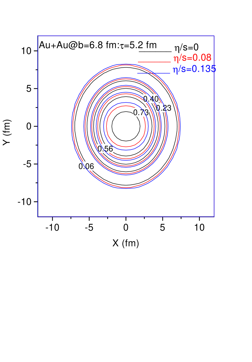
Figure 1: (color online). Contour plots of energy density at (proper) time $\tau$=5.6 fm. The black lines are for ideal fluid ($\eta/s$=0). The red and blue lines are for viscous fluid with ADS/CFT ($\eta/s$=0.08) and perturbative ($\eta/s$=0.135) estimate of viscosity.

VI Results

VI.1 Evolution of the viscous fluid

The energy-momentum conservation equations 9,10,11 are solved using the SHASTA-FCT algorithm. We have made extensive changes to the publicly available code AZHYDRO (described in QGP3 ) for simulation of ideal fluid. The modified code, called ”AZHYDRO-KOLKATA”, simulate the evolution of dissipative fluid, both in 1st and 2nd order theory. In this section we present results of AZHYDRO-KOLKATA for the 1st order theory of dissipative fluid. In the following we will show the results obtain in Au+Au collision at impact parameter $b=$ 6.8 fm, which approximately corresponds to 16-24% centrality Au+Au collisions. With the same initial conditions, we have solved the energy-momentum conservation equations for ideal fluid and viscous fluid.

In Fig.1, we have shown the constant energy density contour plot in x-y plane, after an evolution of 5 fm. The black lines are for ideal fluid evolution. The red and blue lines are for viscous fluid with ADS/CFT ($\eta/s$=0.08) and perturbative ($\eta/s$=0.135) estimate of viscosity. Constant energy density contours, as depicted in Fig.1, indicate that with viscosity fluid cools slowly. Cooling gets slower as viscosity increases. Thus at any point in the x-y plane, viscous fluid temperature is higher than that of the ideal fluid. The results are in accordance with our expectation. For dissipative fluid, ideal equation of motion Eq.21 is changed to,

$$D\varepsilon=-(\varepsilon+p)\nabla_{\mu}u^{\mu}+\pi^{\mu\nu}\nabla_{<\mu}u_{\nu>}\\$$ (53)

Due to viscosity, evolution of energy density is slowed down.

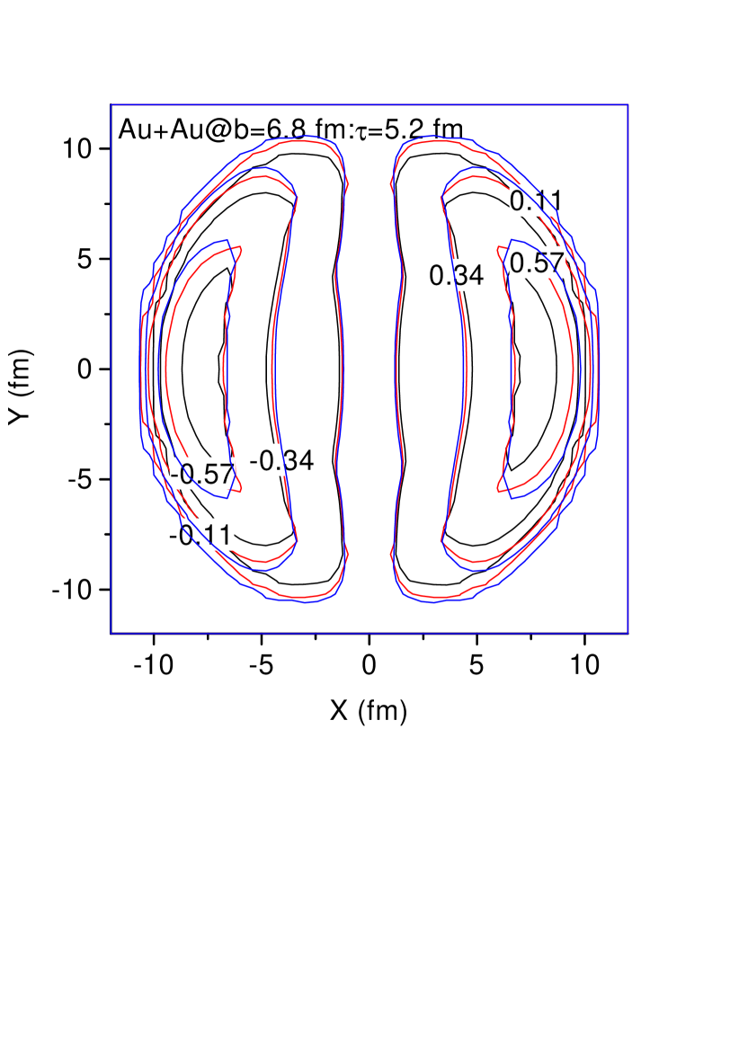
Figure 2: (color online). Contour plots of x-component of fluid velocity $v_{x}$ at $\tau$=5.6 fm. The black lines are for ideal fluid ($\eta/s$=0). The red and blue lines are for viscous fluid with ADS/CFT and perturbative estimate of viscosity, $\eta/s$=0.08 and 0.135.

In Fig.2, we have shown the constant $v_{x}$ contour plot in x-y plane again at $\tau$=5.6 fm. As before the black lines are for the ideal fluid evolution. The red and blue lines are for viscous fluid with $\eta/s$=0.08 and 0.135 respectively. In the central region of the fluid, viscous fluid has more velocity than its ideal counterpart. With viscosity while the energy density evolve slowly, the fluid velocity evolve faster. Contour plot of the y-component of fluid velocity also indicate similar results.

To obtain an idea of transverse expansion of viscous fluid, as opposed to ideal fluid, in Fig.3, we have shown the constant temperature contours in $\tau-x$ plane , at a fixed value of y=0 fm. Transverse expansion is substantially enhanced in a viscous fluid. More the viscosity, more is the transverse expansion. The plot also indicate that at late time, fluid at x=y=0 behaves similarly to a ideal fluid.

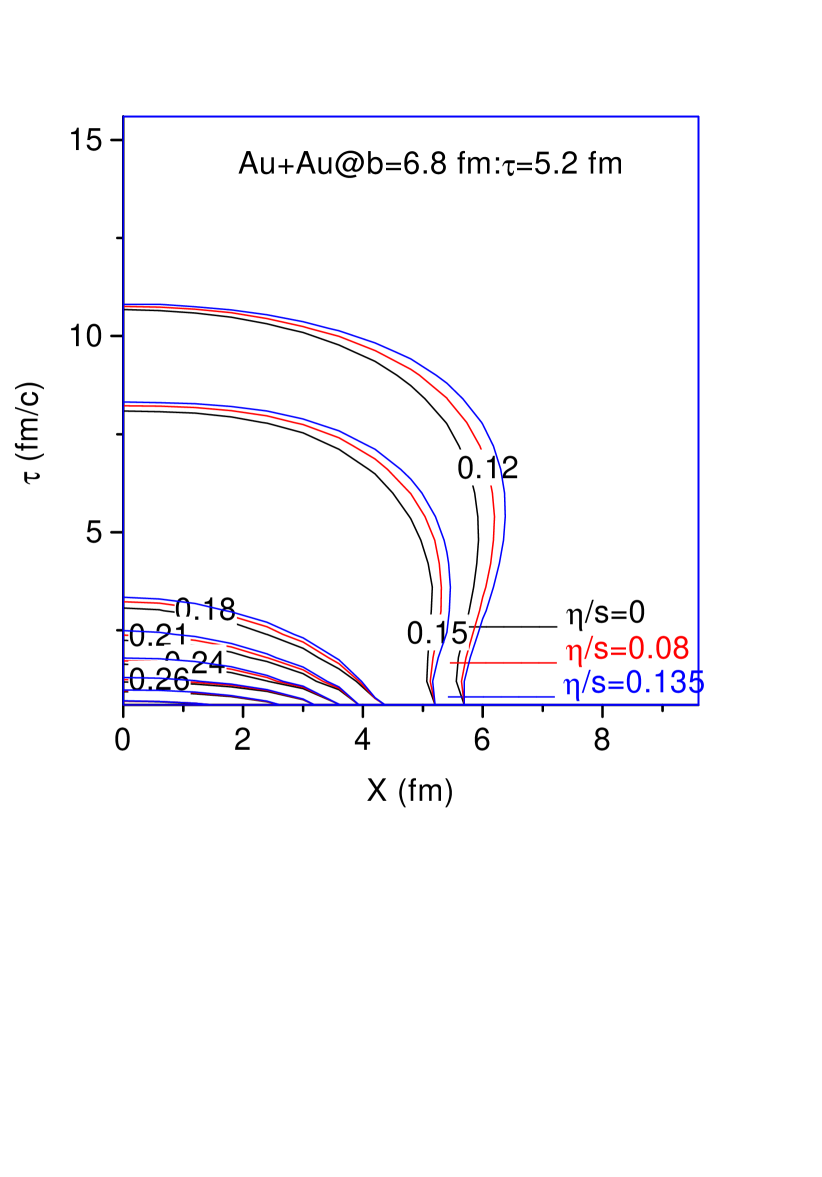
Figure 3: (color online). Contour plots of temperature at y=0 fm in $x-\tau$ plane. The black lines are for ideal fluid ($\eta/s$=0). The red and blue lines are for viscous fluid with $\eta/s$=0.08 and 0.135 respectively.

1st order dissipative theories are acausal. As mentioned earlier, acausality can lead to unphysical behavior like reheating of the fluid in the early stage of evolution MR04 ; Baier:2006um . Do we see any reheating? In Fig.4, the evolution of temperature in viscous dynamics, with perturbative estimate of viscosity ($\eta/s$=0.135) is shown. We have shown the temperature at two positions of the fluid, x=y=0 (the solid line) and x=0,y=3 fm (the dashed line). In both the positions of the fluid, with time as the fluid expands, temperature decreases (as it should be). We find no evidence of reheating. Reheating is not seen also with ADS/CFT estimate of viscosity.

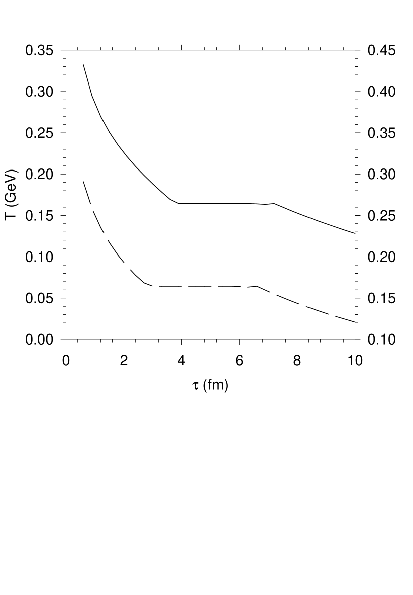
Figure 4: Evolution of the temperature in viscous dynamics with perturbative estimate of viscosity, $\eta/s$=0.135. The solid and dashed lines are for fluid at x=y=0 and x=0,y=3 fm respectively. The x=0,y=3 fm curve is plotted with the right side scale.

In Fig.5, in 4-panels we have shown shear stress tensors $\pi^{\tau\tau}(x,y=0)$, $\tau^{2}\pi^{\eta\eta}(x,y=0)$, $\pi^{xx}(x,y=0)$ and $\pi^{yy}(x,y=0)$ as a function of x. $\eta/s$ =0.135. The solid, long-dashed, dashed and short-dashed lines are for time 0.6, 2.2, 3.2 and 4.2 fm respectively. Initially at $\tau$=0.6 fm, $\pi^{\tau\tau}$ is zero. As the fluid evolve, $\pi^{\tau\tau}$ increases rapidly to a maximum and then decreases. By 4 fm of evolution, it decreases to very small values. We also note that $\pi^{\tau\tau}$ is never very large. The viscous pressures $\tau^{2}\pi^{\eta\eta}$, $\pi^{xx}$ and $\pi^{yy}$ are non-zero at initial time $\tau_{i}$=0.6 fm As the fluid evolve these viscous fluxes rapidly decreases to very small values.

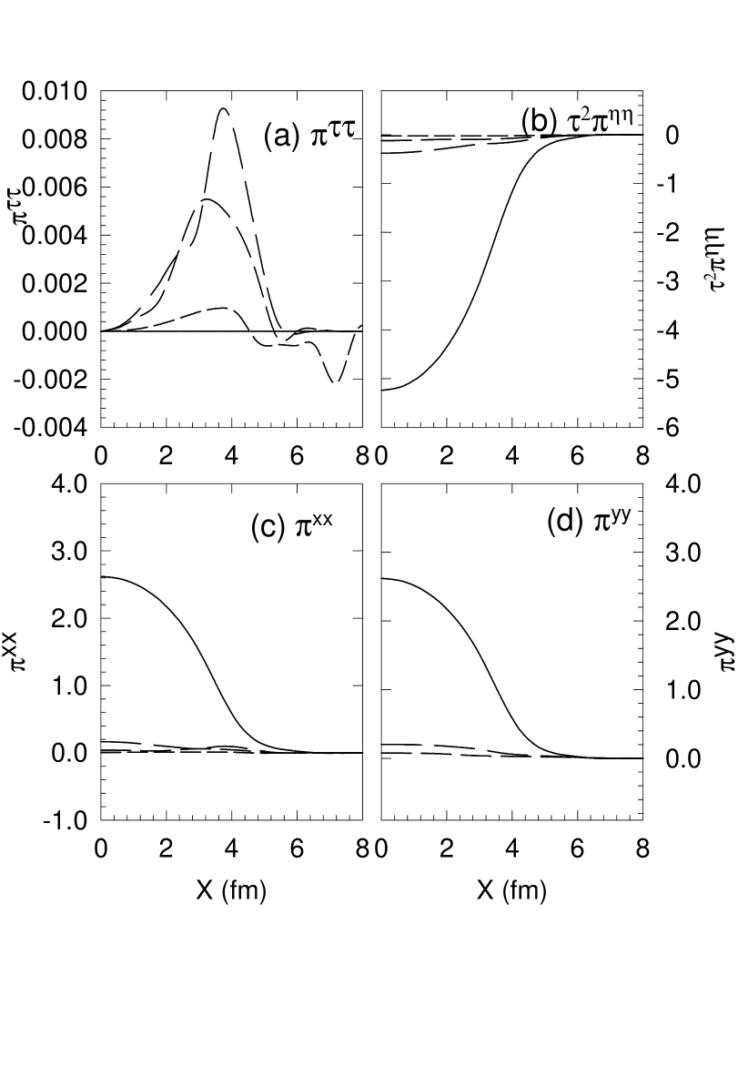
Figure 5: Shear stress tensor $\pi^{\tau\tau}(x,y=0)$, $\tau^{2}\pi^{\eta\eta}(x,y=0)$, $\pi^{xx}(x,y=0)$ and $\pi^{yy}(x,y=0)$ at $\tau$=0.6, 2.2, 3.2 and 4.2 fm are shown in 4 panels.

Viscosity generates entropy. In the model entropy generation due to dissipation can be calculated as,

$$\partial_{\mu}S^{\mu}=\frac{\pi^{\mu\nu}\pi_{\mu\nu}}{2\eta T}$$ (54)

Evolution of spatially average entropy is shown in Fig.6. Entropy generation saturates after $\sim$ 2 fm of evolution. It is expected. As seen in Fig.5, viscous fluxes rapidly decreases and by 2 fm of evolution, the viscous fluxes are decreased sufficiently and do not contribute significantly to the entropy.

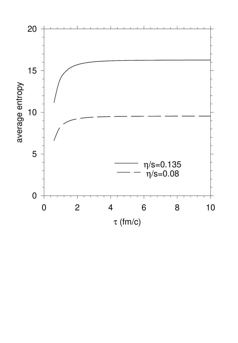
Figure 6: Evolution of average entropy with proper time, for two values of $\eta/s$ is shown.

VI.2 Particle spectra

In this exploratory calculations we have not attempted to fit experimental data. We just exhibit the effect of viscosity on (i) transverse momentum distribution and (ii) elliptic flow of pions. Viscosity influences the particle production by (i) changing the freeze-out surface (freeze-out surface is extended) and (ii) by introducing a correction to the equilibrium distribution function. Non-equilibrium correction to equilibrium distribution function depend, quadratically on the momentum and linearly on the viscous fluxes.

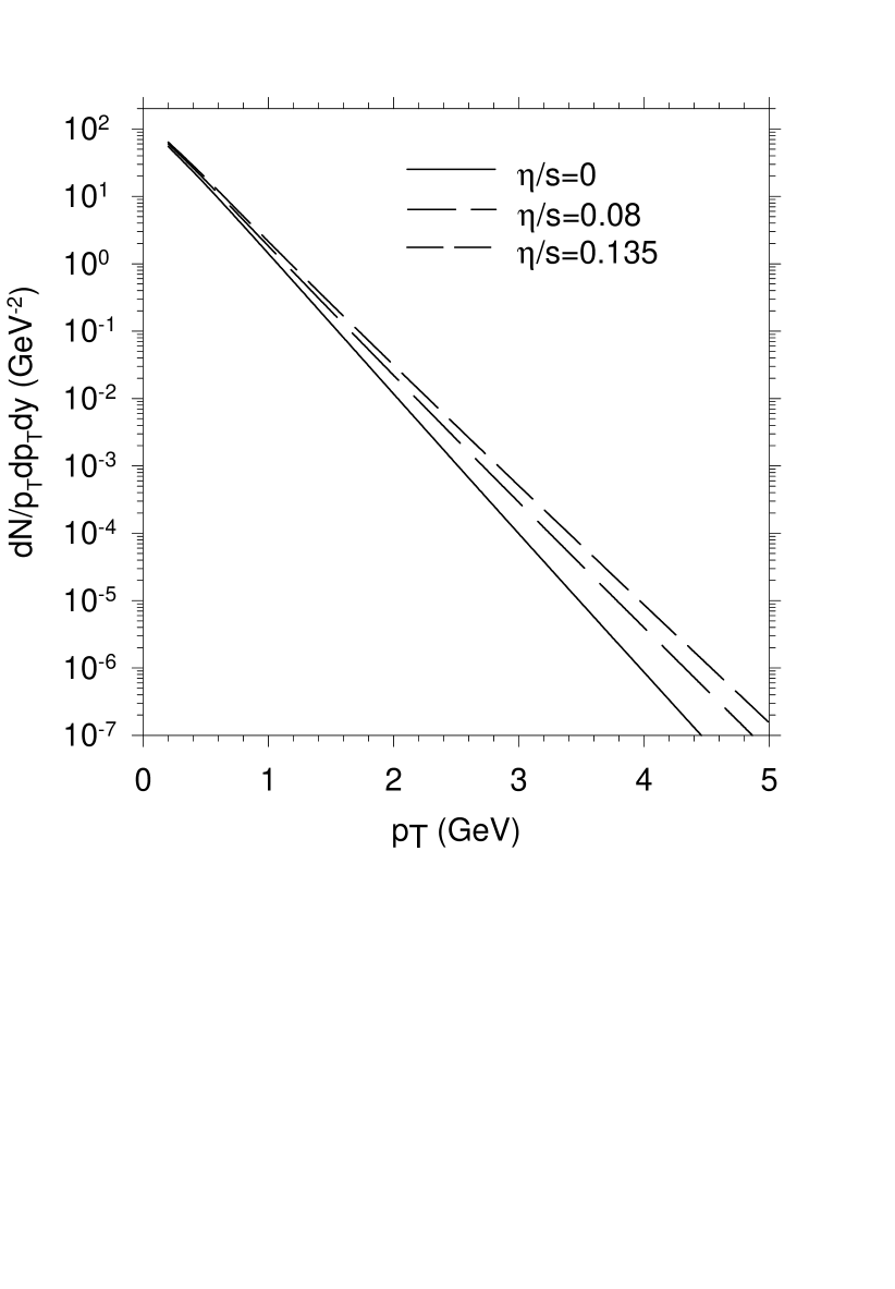
Figure 7: $P_{T}$ distribution of pions. The solid line is for ideal fluid. The long-dashed and medium-dashed lines are for viscous fluid with ADS/CFT ($\eta/s$=0.08) and perturbative ($\eta/s$=0.135) estimate of viscosity. Non-equilibrium correction to equilibrium distribution function is included.

In Fig.7, we have shown the transverse momentum distribution of pions obtained in the Cooper-Frye formalism. Freeze-out temperature is $T_{F}$=0.158 GeV. In this calculation resonance contribution to pion spectra is neglected. Pion production is increased in viscous dynamics. We also note that effect of viscosity is more prominent at large $p_{T}$ than at low $p_{T}$. $p_{T}$ spectra of pions are flattened with viscosity. Particle production increases if viscosity increases. Thus while with ADS/CFT estimate of viscosity, $\eta/s$=0.08, at $p_{T}$ =3 GeV, pion production is increased by a factor 3, with the perturbative estimate of viscosity, $\eta/s$=0.135, the production is increased by a factor of 5. Increase is even more at larger $p_{T}$.

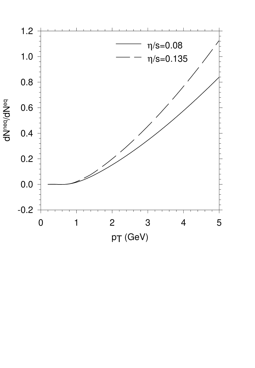
Figure 8: Ratio of correction to particle production due to non-equilibrium distribution to equilibrium distribution function.

We have obtained the non-equilibrium distribution as a correction to the equilibrium distribution function. It is implied that non-equilibrium effects are small and the ratio

$$\frac{dN^{neq}}{dN^{eq}}=\frac{\frac{dN^{neq}}{dyd^{2}p_{T}}}{\frac{dN^{eq}}{dyd^{2}p_{T}}},$$ (55)

is less than 1. In Fig.8, the ratio is shown as a function of $p_{T}$. With ADS/CFT estimate of viscosity, $\eta/s$=0.08, non-equilibrium correction to particle production become comparable to equilibrium contribution beyond $p_{T}$=5 GeV. However, with perturbative estimate, $\eta/s$=0.135, non-equilibrium correction become comparable to or exceeds the equilibrium contribution at $p_{T}$=4.5 GeV. Thus with perturbative estimate of viscosity, hydrodynamic description break down above $p_{T}\sim 4.5GeV$. The blast wave model analysis Teaney:2004qa on the otherhand indicated that viscous dynamics get invalidated beyond $p_{T}\sim$1.7 GeV. The results are not contradictory. In the blast wave model, at the freeze-out, viscosity is quite large, sound attenuation length $\Gamma_{s}\sim$ 1.4 fm. In the present simulation, even for perturbative estimate of viscosity, sound attenuation length at the freeze-out is $\Gamma_{s}\sim 0.2fm$, 7 times smaller than the sound attenuation length used in the blast wave analysis. Naturally, non-equilibrium corrections to equilibrium distribution function remains small over an extended $p_{T}$ range.

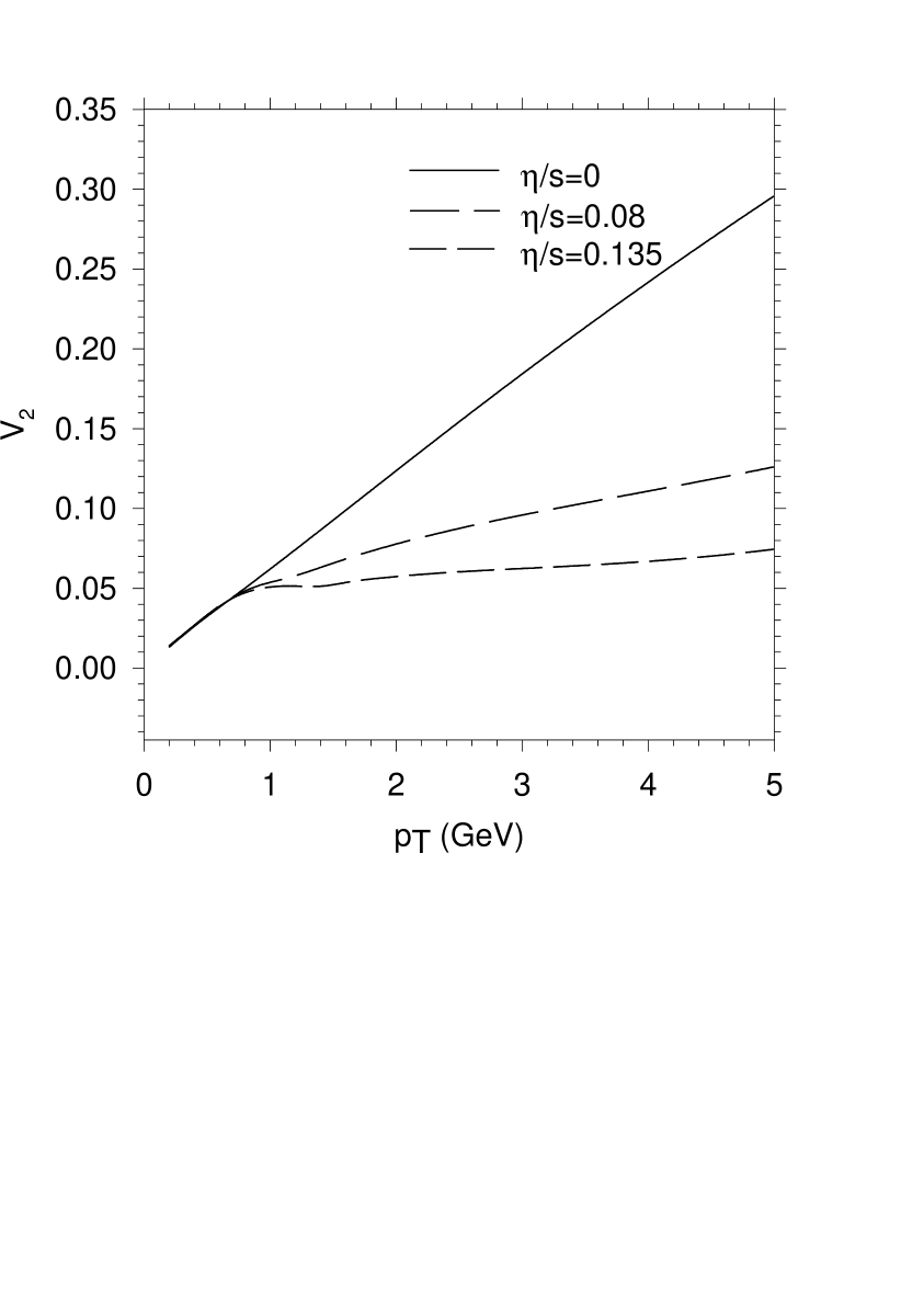
Figure 9: Elliptic flow as a function of transverse momentum. The solid line is for ideal fluid. The long-dashed, medium-dashed and short-dashed lines are for viscous fluid with $\eta/s$=0.08 and 0.135 respectively. Non-equilibrium correction to equilibrium distribution function is included.

We have also calculated the elliptic flow in the model. Being a ratio, elliptic flow is very sensitive to the model. Experimentally, elliptic flow saturates at large $p_{T}$. It is known that ideal fluid does not explain the saturation of elliptic flow. In contrast to experiment, with ideal fluid, elliptic flow continues to increase with $p_{T}$. In Fig.9, we have compared the elliptic flow in ideal and viscous fluid. The solid line is $v_{2}$ for the ideal fluid. The long-dashed and medium-dashed lines are for viscous fluid with ADS/CFT ($\eta/s$=0.08) and perturbative ($\eta/s$=0.135) estimated viscosity. Elliptic flow decreases with viscosity. As viscosity increases, elliptic flow is also reduced. We also note that both for ADS/CFT and perturbative estimate of viscosity, elliptic flow indicate saturation at large $p_{T}$. The result is very encouraging, as experimentally also elliptic flow tends to saturate at large $p_{T}$.

As discussed earlier, ideal fluid dynamics, can explain a large volume of data in Au+Au collisions at RHIC. Our present knowledge about the hot dense matter produced in central Au+Au collisions are obtained from the ideal fluid analysis. As shown in the present paper, QGP fluid, even with ADS/CFT estimate of viscosity $\eta/s$=0.08, generate enough entropy to enhance particle production by a factor of 3 at $p_{T}$=3 GeV. Naturally, if QGP fluid is viscous, initial conditions as required to explain RHIC data with ideal fluid dynamics will overpredict the experimental $p_{T}$ distribution. Viscous fluid dynamics will require much less initial temperature than an ideal fluid to explain the same $p_{T}$ spectra. As an example, in Fig.10, we have compared the pion spectra obtained in viscous dynamics with ADS/CFT estimate of viscosity ($\eta/s$=0.08), initialised with entropy density of 110,80, and 60 $fm^{-3}$ with the pion spectra obtained in an ideal fluid dynamics, initialised with entropy density s=110 $fm^{-3}$. For all the fluids, the initial time is $\tau_{i}$=0.6 fm and freeze-out temperature is 158 MeV. Viscous fluid initialised with entropy density between 60-80 $fm^{-3}$, compare well with the pion spectra from ideal fluid initialised at much higher entropy density. To produce the same pion spectra, while ideal fluid require a initial temperature of 350 MeV, the viscous fluid require much less temperature between 270-290 MeV. The ideal fluid dynamics can overestimate the initial temperature of fluid produced in Au+Au collisions at RHIC by 20-30%.

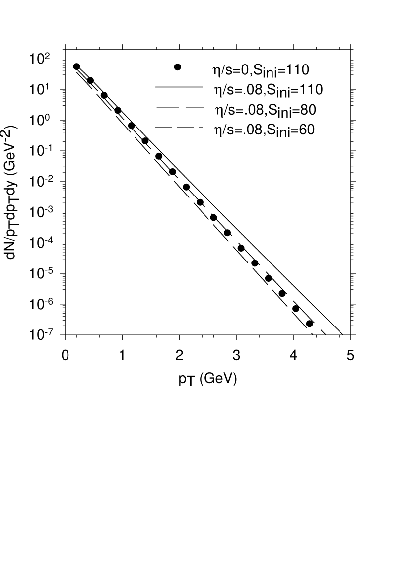
Figure 10: The solid circle is the $p_{T}$ distribution obtained in ideal fluid dynamics, with initial entropy density s=110$fm^{-3}$. The solid, long dashed and dashed lines are for viscous fluid with ADS/CFT estimate of viscosity, $\eta/s$=0.08, initialised at entropy density s=60,80 and 110 $fm^{-3}$ respectively. Non-equilibrium correction to equilibrium distribution function is included.

VII Summary and conclusions

We have studied the boost-invariant hydrodynamic evolution of QGP fluid with dissipation due to shear viscosity. In this study we have employed the 1st order theory of dissipative relativistic fluid. 1st order theories suffer from the problem of causality, signal can travel faster than light. Unphysical effects like reheating of the fluid, early in the evolution, can occur. However, for a fluid like QGP, where viscosity is small, with appropriate initial conditions, effects of causality violation can be minimised. In this model study, we have considered two values of viscosity, the ADS/CFT motivated value, $\eta/s\approx$0.08 and perturbatively estimated viscosity, $\eta/s\approx$0.135. Both the ideal and viscous fluids are initialised similarly. At the initial time $\tau_{i}$=0.6 fm, initial central entropy density is 110 $fm^{-3}$, with transverse profile taken from a Glauber model calculation. Viscous hydrodynamics require initial conditions for the shear-stress tensor components. It is assumed that at the equilibration time, the shear stress tensors components have reached their boost-invariant values. The initial conditions of the fluid are such that for both the values of viscosity ($\eta/s$=0.08 and 0.135), the condition of validity of viscous hydrodynamics, $\Gamma_{s}/\tau<<1$ is satisfied all through the evolution. Explicit simulation of ideal and viscous fluids confirms that energy density of a viscous fluid, evolve slowly than its ideal counterpart. The fluid velocities on the other hand evolve faster in viscous dynamics than in ideal dynamics. Transverse expansion is also more in viscous dynamics. For a similar freeze-out condition freeze-out surface is extended in viscous fluid.

We have also studied the effect of viscosity on particle production. Viscosity generates entropy leading to enhanced particle production. Particle production is increased due to (i) extended freeze-out surface and (ii) non-equilibrium correction to equilibrium distribution function. Non-equilibrium correction to equilibrium distribution function is a dominating factor influencing the particle production at large $p_{T}$. With ADS/CFT (perturbative) estimate of viscosity, at $p_{T}$=3 GeV, pion production is increased by a factor 3 (5) . Increase is even more at large $p_{T}$. While viscosity enhances particle production, it reduces the elliptic flow. At $p_{T}$=3 GeV, for ADS/CFT(perturbative) estimate of viscosity, elliptic flow is reduced by a factor of 2(3). We also find that at large $p_{T}$ elliptic flow tends to saturate.

To conclude, present study shows viscosity, even if small, can be very important in analysis of RHIC Au+Au collisions. Currently accepted initial temperature of hot dense matter produced in RHIC Au+Au collisions, obtained from ideal fluid analysis can be changed by 20% or more with dissipative dynamics.

- (1) BRAHMS Collaboration, I. Arsene et al., Nucl. Phys. A 757, 1 (2005).
- (2) PHOBOS Collaboration, B. B. Back et al., Nucl. Phys. A 757, 28 (2005).
- (3) PHENIX Collaboration, K. Adcox et al., Nucl. Phys. A 757 (2005), in press [arXiv:nucl-ex/0410003].
- (4) STAR Collaboration, J. Adams et al., Nucl. Phys. A 757 (2005), in press [arXiv:nucl-ex/0501009].
- (5) P. F. Kolb and U. Heinz, in Quark-Gluon Plasma 3, edited by R. C. Hwa and X.-N. Wang (World Scientific, Singapore, 2004), p. 634.
- (6) U. Heinz, J. Phys. G 31, S717 (2005).
- (7) C. Eckart, Phys. Rev. 58, 919 (1940).
- (8) L. D. Landau and E. M. Lifshitz, Fluid Mechanics, Sect. 127, Pergamon, Oxford, 1963.
- (9) W. Israel, Ann. Phys. (N.Y.) 100, 310 (1976); W. Israel and J. M. Stewart, Ann. Phys. (N.Y.) 118, 349 (1979).
- (10) D. A. Teaney, J. Phys. G 30, S1247 (2004). Phys. Rev. C 68, 034913 (2003) [arXiv:nucl-th/0301099].
- (11) A. Muronga, Phys. Rev. Lett. 88, 062302 (2002) [Erratum ibid. 89, 159901 (2002)]; and Phys. Rev. C 69, 034903 (2004).
- (12) A. Muronga and D. H. Rischke, nucl-th/0407114 (v2).
- (13) A. K. Chaudhuri and U. Heinz, nucl-th/0504022.
- (14) U. W. Heinz, H. Song and A. K. Chaudhuri, Phys. Rev. C 73, 034904 (2006) [arXiv:nucl-th/0510014].
- (15) K. Kajantie, Nucl. Phys. A 418, 41C (1984). G. Baym, Nucl. Phys. A 418, 525C (1984). A. Hosoya and K. Kajantie, Nucl. Phys. B 250, 666 (1985). A. K. Chaudhuri, J. Phys. G 26, 1433 (2000) [arXiv:nucl-th/9808074]. A. K. Chaudhuri, Phys. Scripta 61, 311 (2000) [arXiv:nucl-th/9705047]. A. K. Chaudhuri, Phys. Rev. C 51, 2889 (1995).
- (16) R. Baier, P. Romatschke and U. A. Wiedemann, arXiv:hep-ph/0602249.
- (17) P. Arnold, G. D. Moore and L. G. Yaffe, JHEP 0011, 001 (2000) [arXiv:hep-ph/0010177].
- (18) G. Baym, H. Monien, C. J. Pethick and D. G. Ravenhall, Phys. Rev. Lett. 64, 1867 (1990).
- (19) G. Policastro, D. T. Son and A. O. Starinets, Phys. Rev. Lett. 87, 081601 (2001) [arXiv:hep-th/0104066].
- (20) G. Policastro, D. T. Son and A. O. Starinets, JHEP 0209, 043 (2002) [arXiv:hep-th/0205052].