Coleman-Weinberg mechanism for spontaneous chiral symmetry breaking in the massless chiral sigma model

Abstract

We study the effect of one-loop corrections from nucleon together with those from boson in the massless chiral sigma model, where we perform the Coleman-Weinberg renormalization procedure. This renormalization procedure has a mechanism of spontaneous symmetry breaking due to radiative corrections in $\phi^{4}$ theory. We apply it to the system of nucleon and bosons with chiral symmetry where the negative-mass term of bosons does not exist. Spontaneous chiral symmetry breaking is derived from the contribution of nucleon and boson loops which generates the masses of nucleon, scalar meson, and vector meson dynamically. We find that the renormalization scale plays an important role for the breaking of the symmetry between fermion (nucleon) and boson, and eventually for the chiral symmetry at the same time. In addition, we find that the naturalness restores by means of the introduction of the vacuum fluctuation from both nucleon and boson. Finally we obtain a stable effective potential with the effect of Dirac sea in the chiral model for the first time.

I Introduction

The relativistic mean field (RMF) approximation is very popular now for the description of nuclei and nuclear matter. The success of the RMF model originates from the presence of large scalar and vector potentials with opposite sign walecka . The scalar potential is attractive and proportional to the scalar density, while the vector potential is repulsive and proportional to the vector density. This fact makes the net potential attractive for small densities and repulsive for large densities, the feature of which provides the saturation property of nuclear matter. The large scalar and vector potentials with opposite sign provide a large spin-orbit potential, which is necessary to provide the jj-closed shell magic numbers meyerjensen . Further introduction of non-linear terms of the sigma meson field with a few additional parameters is able to make the incompressibility appropriate and describe nuclei quantitatively in the entire mass region rheinhard ; sugahara ; lalazisis .

In principle, however, we have to include the contribution of negative-energy states to the total energy and the densities due to the modification of the negative-energy states caused by formation of the nucleus. This is because the nucleons with positive energy polarize the negative-energy states and the whole object including the negative-energy nucleons should be the nucleus of our concern. In the development of the RMF model, we have assumed that the parameters in the RMF Lagrangian mocks up the contribution from negative-energy states. In this sense, the present RMF model is simply not more than a phenomenological model. Definitely, there are several works to try to include the contribution of negative-energy states walecka ; greiner ; nagata .

A theoretical study of the RMF model of the nucleus was performed by using the sigma model of Gell-mann and Levy gellmann . The use of the original Lagrangian after making the Weinberg transformation in addition to the introduction of the omega meson term was not successful to generate a good saturation property of nuclear matter in the mean field approximation boguta1 . Hence, the chiral model was modified by introducing the dynamical mass generation term for the omega meson as the case of the nucleon. This modified sigma model, named as chiral sigma model, is able to provide a good saturation property for nuclear matter boguta1 ; ogawa1 . However, the incompressibility comes out to be too large (K=650[MeV]), which causes a bad feature in the single particle spectra of finite nuclei ogawa1 .

This observation sets a stage to study the modification of negative-energy states, since the linear sigma model Lagrangian is used for the hadron properties and for pion dynamics. Hence, we study the effect of the Dirac sea in the chiral sigma model for nuclear structure. The chiral sigma model is renormalizable, and it is legitimate to include the Dirac sea in this model. In the non-chiral model (Walecka model) it is known that the contribution of the Dirac sea is to make the scalar density decrease by about 10% to 20% at the saturation density and reduces the incompressibility nagata . We shall try now to include the Dirac sea in the chiral sigma model. Since the chiral sigma model has the chiral symmetry, the counter terms need to respect this symmetry matsui . We obtain the counterterms with the chiral symmetry, but the counterterms remain arbitrary and the total effective potential comes out to be unstable boguta2 . We should reconstruct one-loop corrections with chiral symmetry using a new renormalization procedure and the mechanism of the spontaneous symmetry breaking. This is the purpose of this paper.

In Sect. II, we review the radiative corrections as the origin of spontaneous symmetry breaking in the Coleman-Weinberg scheme coleman . Using the Coleman-Weinberg renormalization scheme, we calculate the one-loop corrections with chiral symmetry and construct the massless chiral sigma model with Dirac sea in Sect. III. In Sect. IV and V, we show some properties of the massless chiral sigma model. We summarize the present study in Sect. VI.

II Radiative corrections and spontaneous symmetry breaking

The chiral model usually has a mechanism of spontaneous chiral symmetry breaking by construction. This mechanism comes from the negative-mass term of (Higgs) bosons to make a minimum point in the wine bottle potential. First, we review the radiative corrections of this system in the $\phi^{4}$ theory. The Lagrangian is

$$\mathcal{L}=\frac{1}{2}(\partial_{\mu}\phi)^{2}-\frac{\mu^{2}}{2}\phi^{2}-\frac{\lambda}{4!}\phi^{4}-\delta\mathcal{L}_{CTC}.$$ (1)

This Lagrangian consists of only the field $\phi$ for scalar meson, and $\mu^{2}$, $\lambda$ are the mass and the coupling constant. The last term $\delta\mathcal{L}_{CTC}$ is the counterterm Lagrangian, which is necessary to renormalize the boson loop in Fig. 1.

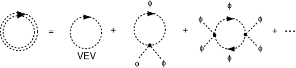
Figure 1: All-order boson loop corrections at the one-loop level. First term of the right hand side is the vacuum expectation value (VEV) corresponding to the contribution from the valence bosons. The second and the third terms are the higher order corrections of VEV.

The effective action of Eq. (1) at the one-loop level can be written as

$$\Gamma^{B} = \int d^{4}x\left[\frac{i}{2}\mathop{\mathrm{Tr}}\nolimits\ln\left(p^{2}-\mu^{2}-\frac{\lambda}{2}\phi^{2}\right)-VEV+\mathcal{L}\right]$$ (2)

$$= \int d^{4}x\left[-V_{B}^{R}(\phi)+\frac{1}{2}\left(1+Z_{\phi}(\phi)\right)(\partial_{\mu}\phi)^{2}+Y_{\phi}(\phi)(\partial_{\mu}\phi)^{4}+\cdots\right].$$

We take ordinary renormalization conditions for mass, coupling constant, and derivative term to Eq. (2) with counterterms,

$$\left.\frac{\partial^{2}V_{B}^{R}}{\partial\phi^{2}}\right|_{\phi=0} = \mu^{2},$$ (3)

$${}\left.\frac{\partial^{4}V_{B}^{R}}{\partial\phi^{4}}\right|_{\phi=0} = \lambda,$$ (4)

$${}Z_{\phi}|_{\phi=0} = 0.$$ (5)

Here, we keep only the lowest order derivative term, since the derivative expansion is known to converge rapidly greiner ; fraser ; haga . Therefore we obtain the renormalized Lagrangian as,

$$\mathcal{L} = \frac{1}{2}\left(1+Z_{\phi}\right)(\partial_{\mu}\phi)^{2}-V_{B}^{R},$$ (6)

where

$$V_{B}^{R} = \frac{\mu^{2}}{2}\phi^{2}+\frac{\lambda}{4!}\phi^{4}$$ (7)

$$+\frac{\mu^{4}}{64\pi^{2}}\left[\left(1+\frac{\lambda\phi^{2}}{2\mu^{2}}\right)^{2}\ln\left(1+\frac{\lambda\phi^{2}}{2\mu^{2}}\right)-\frac{\lambda\phi^{2}}{2\mu^{2}}-\frac{3}{2}\left(\frac{\lambda\phi^{2}}{2\mu^{2}}\right)^{2}\right],$$

$${}Z_{\phi} = \frac{\lambda^{2}\phi^{2}}{192\pi^{2}\left(\mu^{2}+\frac{1}{2}\lambda\phi^{2}\right)}.$$ (8)

This potential has a mechanism to break the spontaneous symmetry owing to the negative-mass term ($\mu^{2}<0$). This is the standard spontaneous symmetry breaking scheme.

We introduce now the Coleman-Weinberg renormalization scheme coleman . In the Coleman-Weinberg scheme, we set the mass term vanish and let the radiative corrections have the same role as the negative-mass term. We change the renormalization conditions from (3) $\sim$ (5) to the new ones as,

$$\left.\frac{\partial^{2}V_{B}^{R}}{\partial\phi^{2}}\right|_{\phi=0} = 0,$$ (9)

$${}\left.\frac{\partial^{4}V_{B}^{R}}{\partial\phi^{4}}\right|_{\phi=m} = \lambda,$$ (10)

$${}Z_{\phi}|_{\phi=m} = 0,$$ (11)

where we introduce the renormalization scale $m$ to Eqs. (10) and (11) in order to avoid the logarithmic singularity at the origin of the effective potential. Finally the renormalized effective potential becomes

$$V_{B}^{R} = \frac{\lambda}{4!}\phi^{4}+\frac{\lambda^{2}\phi^{4}}{256\pi^{2}}\left[\ln\left(\frac{\phi^{2}}{m^{2}}\right)-\frac{25}{6}\right],$$ (12)

with the constant correction $\frac{\lambda}{96\pi^{2}}$ in $Z_{\phi}$ before the renormalization, which is removed by the counterterm. Since the second term of Eq. (12) is negative around the origin, it has an effect to make a new minimum at some point away from the origin. This mechanism plays the role of spontaneous symmetry breaking in the Coleman-Weinberg scheme. This scheme is not used, however, in the actual case, since the radiative corrections are much bigger than the tree level contributions.

III One-loop corrections with chiral symmetry

It is well known that chirally symmetric renormalization in the conventional way gives unstable effective potential boguta2 and too large non-linear interactions furn . These features come from the form of the counterterms and the renormalization conditions. In order to respect the chiral symmetry of the model, the number of the counterterms is restricted to two terms despite of four divergent diagrams of the nucleon loop. After spontaneous chiral symmetry breaking, we take only two renormalization conditions for a local minimum and the mass in the ordinary way matsui ; lee . In this way the coupling constant $\lambda$ could not be renormalized properly.

Boson-loop corrections were, then, introduced for the cancellation of the unstable effective potential coming from the nucleon loop jackson ; lee . We have to take a large sigma meson mass as about 1125 MeV in order to achieve the cancellation of the nucleon and the boson loop corrections. In this case, we get too small scalar potential and eventually too small spin-orbit splitting for the case of the nucleus. In addition, the problem of instability is not solved perfectly. Hence, until now, we do not have a satisfactory procedure to treat the vacuum polarization for the Lagrangian with the chiral symmetry.

We consider now the Coleman-Weinberg renormalization scheme to both the nucleon and boson loops with chiral symmetry. As shown in the previous section, radiative corrections from boson are taken into account before symmetry breaking and give rise to the spontaneous symmetry breaking. We consider then one-loop corrections for nucleon before the spontaneous chiral symmetry breaking in the same way as the boson loop in the $\phi^{4}$ theory.

We begin with the chiral sigma model boguta1 ; ogawa1 :

$$\mathcal{L} = \bar{\psi}\left[i\gamma_{\mu}\partial^{\mu}-g_{\sigma}(\phi+i\gamma_{5}\bm{\tau}\cdot\bm{\pi})-g_{\omega}\gamma_{\mu}\omega^{\mu}\right]\psi$$ (13)

$$+ \frac{1}{2}\left(\partial_{\mu}\phi\partial^{\mu}\phi+\partial_{\mu}\bm{\pi}\cdot\partial^{\mu}\bm{\pi}\right)-\frac{\mu^{2}}{2}\left(\phi^{2}+\bm{\pi}^{2}\right)-\frac{\lambda}{4}\left(\phi^{2}+\bm{\pi}^{2}\right)^{2}$$

$$- \frac{1}{4}\Omega_{\mu\nu}\Omega^{\mu\nu}+\frac{1}{2}{}\widetilde{g_{\omega}}^{2}\left(\phi^{2}+\bm{\pi}^{2}\right)\omega_{\mu}\omega^{\mu}-\delta\mathcal{L}_{CTC},$$

where $\psi$, $\phi$, and $\bm{\pi}$ are nucleon field, sigma meson field, and pi meson field, respectively. This Lagrangian has the chiral symmetry. The sigma meson field appears together with the pion field in the chiral symmetric way. There does not exist the nucleon mass term, which is produced by chiral symmetry breaking in this chiral sigma model. We introduce omega meson field, $\omega_{\mu}$, in order to generate an appropriate repulsive effect to obtain a stable nucleus. The coupling constant $g_{\omega}$ is therefore considered to be a free parameter. The omega meson acquires its mass by chiral symmetry breaking as the case of the nucleon field boguta1 ; ogawa1 . The field strength of the isoscalar vector meson is given by

$$\Omega_{\mu\nu}=\partial_{\mu}\omega_{\nu}-\partial_{\nu}\omega_{\mu}.$$ (14)

Up to this stage this Lagrangian has a mass term $\mu^{2}$ of scalar bosons. We take the limit $\mu^{2}\rightarrow 0$ in the Coleman-Weinberg renormalization procedure. In this sense we name it the massless chiral sigma model (MCSM). We describe $\phi$ for the scalar field before the chiral symmetry breaking and $\sigma$ after the chiral symmetry breaking hereafter.

III.1 Boson loop with chiral symmetry

We expect that the boson loop effective potential with chiral symmetry is almost the same as the one in the previous section. It is necessary to consider new diagrams with different bosons as shown in Fig. 2.

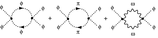
Figure 2: For the four external lines of sigma meson, for example, three-type diagrams exist.

In order to respect the chiral symmetry we must deal with sigma and pi meson equally. The effective action becomes

$$\Gamma_{B}^{\chi} = \int d^{4}x\left[\frac{i}{2}\ln\det\left(-\frac{\delta^{2}\mathcal{L}}{\delta b\delta b}\right)-VEV-\delta\mathcal{L}_{CTC}^{B}\right]$$ (15)

$$= \int d^{4}x\left[-V_{B}^{R}(\phi,\bm{\pi})+\frac{1}{2}Z_{\sigma\pi}^{B}(\partial_{\mu}\phi\partial^{\mu}\phi+\partial_{\mu}{\bm{\pi}}\cdot\partial^{\mu}{\bm{\pi}})+\cdots\right],$$

where $\mathcal{L}$ includes the tree contribution and $\delta\mathcal{L}^{B}_{CTC}$ is the counterterms for the boson loop. $\frac{\delta^{2}\mathcal{L}}{\delta b\delta b}$ means the second functional derivatives of $\mathcal{L}$ with respect to bosons (sigma, pi, and omega mesons). Here we can neglect the external lines of vector meson owing to the current conservation. For simplicity we introduce the new variable,

$$\rho^{2}=\phi^{2}+{\bm{\pi}}^{2}.$$ (16)

We change the renormalization conditions for Eq. (15) using its variable as

$$\left.\frac{\partial^{2}V_{B}^{R}}{\partial\rho^{2}}\right|_{\rho^{2}=0} = 0,$$ (17)

$${}\left.\frac{\partial^{4}V_{B}^{R}}{\partial\rho^{4}}\right|_{\rho^{2}=m^{2}} = 0,$$ (18)

$${}\left.Z_{\sigma\pi}^{B}\right|_{\rho^{2}=m^{2}} = 0.$$ (19)

Finally the renormalized potential of boson with the chiral symmetry becomes

$$V_{B}^{R} = \frac{\rho^{4}}{256\pi^{2}}\left[(6\lambda)^{2}\left\{1+3\left(\frac{1}{3}\right)^{2}\right\}+12\widetilde{g_{\omega}}^{4}\right]\left[\ln\left(\frac{\rho^{2}}{m^{2}}\right)-\frac{25}{6}\right]$$ (20)

$$= \frac{3\rho^{4}}{64\pi^{2}}\left(4\lambda^{2}+\widetilde{g_{\omega}}^{4}\right)\left[\ln\left(\frac{\rho^{2}}{m^{2}}\right)-\frac{25}{6}\right]$$

$$= \frac{3\left(4\lambda^{2}+\widetilde{g_{\omega}}^{4}\right)}{64\pi^{2}}(\phi^{2}+{\bm{\pi}}^{2})^{2}\left[\ln\left(\frac{\phi^{2}+{\bm{\pi}}^{2}}{m^{2}}\right)-\frac{25}{6}\right].$$

The calculation is entirely analogous to Eq. (12). We only need to note that the $\phi^{2}{\bm{\pi}}^{2}$ coupling is $1/3$ of the $\phi^{4}$ coupling and there are three kinds of pion and that the extra factor 12 in the omega loop comes from the trace of Lorentz-gauge propagator and coupling constant. In the same way we calculate the coefficients of derivative terms by including all contributions from boson and find before the renormalization,

$$Z_{\sigma\pi}^{B}=\frac{2\lambda+\widetilde{g_{\omega}}^{2}}{16\pi^{2}}.$$ (21)

This constant correction is removed by taking a counterterm to cancel out. Hence, we have $Z_{\sigma\pi}^{B}=0$ eventually.

III.2 Nucleon loop with chiral symmetry

It is important to take into account the nucleon loop before the chiral symmetry breaking since the chiral symmetry is fulfilled only in the massless phase. However we encounter the same difficulty like the logarithmic singularity of boson loop in the massless limit. At first we calculate the nucleon loop with finite mass in the same way as the boson loop. Then we take the limit of massless phase ($M\rightarrow 0$) and replace $\sigma$ with $\phi$ at the same time in the renormalization procedure. The one-loop effective action of nucleon with chiral symmetry is given by

$$\Gamma_{F}^{\chi} = \int d^{4}x\left[-i\mathop{\mathrm{Tr}}\nolimits\ln\left\{/{k}-M-g_{\sigma}(\sigma+i\gamma_{5}\bm{\tau}\cdot\bm{\pi})-g_{\omega}\gamma_{\mu}\omega^{\mu}\right\}-VEV-\delta\mathcal{L}^{F}_{CTC}\right]$$ (22)

$$= \int d^{4}x\left[-V_{F}^{R}(\phi,\bm{\pi})+\frac{1}{2}Z_{\sigma\pi}^{F}(\partial_{\mu}\phi\partial^{\mu}\phi+\partial_{\mu}{\bm{\pi}}\cdot\partial^{\mu}{\bm{\pi}})+\frac{1}{4}Z_{\omega}^{F}\Omega_{\mu\nu}\Omega^{\mu\nu}+\cdots\right],$$

where $\delta\mathcal{L}^{F}_{CTC}$ is the counterterms for nucleon loop.

Figure 3: Nucleon loop potential in the relativistic mean field (RMF) approximation. Double line is nucleon propagator with RMF and includes all-order scalar, pseudoscalar, and vector potentials from Dyson equation. Note that the contributions of nucleon loops coupled with odd-order pion couplings vanish due to the property of $\gamma_{5}$. First term in right hand side means vacuum expectation value (VEV) corresponding to the loop contribution from the valence nucleon.

In the calculation it is important to consider the one-nucleon loop contribution in the massless phase. In the phase of the chiral symmetry breaking the diagrams from sigma meson are different from ones from pi meson due to the property of pseudoscalar coupling in Fig. 3. However we can deal with both sigma and pi mesons symmetrically before the chiral symmetry breaking. We take the renormalization conditions for Eq. (22) using new variable

$$\left.\frac{\partial^{2}V_{F}^{R}}{\partial\rho^{2}}\right|_{\rho^{2}=0} = 0,$$ (23)

$${}\left.\frac{\partial^{4}V_{F}^{R}}{\partial\rho^{4}}\right|_{\rho^{2}=m^{2}} = 0,$$ (24)

$${}\left.Z_{\sigma\pi}^{F}\right|_{\rho^{2}=m^{2}} = 0,$$ (25)

$${}\left.Z_{\omega}^{F}\right|_{\rho^{2}=m^{2}} = 0.$$ (26)

Using these conditions we obtain the renormalized potential of nucleon loop as

$$V_{F}^{R} = -\frac{g_{\sigma}^{4}\rho^{4}}{8\pi^{2}}\left[\ln\left(\frac{\rho^{2}}{m^{2}}\right)-\frac{25}{6}\right]$$ (27)

$$= -\frac{g_{\sigma}^{4}}{8\pi^{2}}(\phi^{2}+{\bm{\pi}}^{2})^{2}\left[\ln\left(\frac{\phi^{2}+{\bm{\pi}}^{2}}{m^{2}}\right)-\frac{25}{6}\right],$$

$${}Z_{\sigma\pi}^{F} = -\frac{g_{\sigma}^{2}}{4\pi^{2}}\ln\left(\frac{\phi^{2}+\bm{\pi}^{2}}{m^{2}}\right),$$ (28)

$${}Z_{\omega}^{F} = \frac{g_{\omega}^{2}}{6\pi^{2}}\ln\left(\frac{\phi^{2}+\bm{\pi}^{2}}{m^{2}}\right).$$ (29)

In the same way as the boson loop, we also introduce the same renormalization scale $m$ in order to avoid a logarithmic singularity. As one can see in Eqs. (20) and (27), the difference between boson and fermion loops is sign and coupling constant, but both of them have the same function forms. This is true before chiral symmetry breaking and by using this renormalization procedure we can deal with the loop contributions from the boson and nucleon symmetrically. Through these good features we define the absolute ratio of $V_{B}^{R}$ to $V_{F}^{R}$ in order to estimate the loop corrections from boson and nucleon,

$$\gamma=\left|\frac{V_{B}^{R}}{V_{F}^{R}}\right|=\frac{3\left(4\lambda^{2}+\widetilde{g_{\omega}}^{4}\right)}{8g_{\sigma}^{4}}.$$ (30)

It is possible to obtain the total renormalized potential using this ratio as

$$V_{all}^{R}=V_{B}^{R}+V_{F}^{R}=\frac{\gamma-1}{8\pi^{2}}g_{\sigma}^{4}(\phi^{2}+{\bm{\pi}}^{2})^{2}\left[\ln\left(\frac{\phi^{2}+{\bm{\pi}}^{2}}{m^{2}}\right)-\frac{25}{6}\right].$$ (31)

III.3 Total Lagrangian and spontaneous chiral symmetry breaking

In the above two subsections, we have obtained the renormalized one-loop potential of boson and nucleon with the chiral symmetry. The massless chiral sigma model with Eq. (31) becomes

$$\mathcal{L}^{MCSM} = \bar{\psi}\left[i\gamma_{\mu}\partial^{\mu}-g_{\sigma}(\phi+i\gamma_{5}{\bm{\tau}}\cdot{\bm{\pi}})-g_{\omega}\gamma_{\mu}\omega^{\mu}\right]\psi$$ (32)

$$+ \frac{1}{2}\left(\partial_{\mu}\phi\partial^{\mu}\phi+\partial_{\mu}{\bm{\pi}}\cdot\partial^{\mu}{\bm{\pi}}\right)-\frac{\lambda}{4}(\phi^{2}+{\bm{\pi}}^{2})^{2}$$

$$- \frac{1}{4}\Omega_{\mu\nu}\Omega^{\mu\nu}+\frac{1}{2}\widetilde{g_{\omega}}^{2}(\phi^{2}+{\bm{\pi}}^{2})\omega_{\mu}\omega^{\mu}$$

$$- \frac{\gamma-1}{8\pi^{2}}g_{\sigma}^{4}(\phi^{2}+{\bm{\pi}}^{2})^{2}\left[\ln\left(\frac{\phi^{2}+{\bm{\pi}}^{2}}{m^{2}}\right)-\frac{25}{6}\right]$$

$$+ \frac{1}{2}Z_{\sigma\pi}\left(\partial_{\mu}\phi\partial^{\mu}\phi+\partial_{\mu}{\bm{\pi}}\cdot\partial^{\mu}{\bm{\pi}}\right)+\frac{1}{4}Z_{\omega}\Omega_{\mu\nu}\Omega^{\mu\nu}$$

$$+ \epsilon\phi.$$

Here, we have added the explicit chiral symmetry breaking term, $\epsilon\phi$, which produces the finite pion mass after chiral symmetry breaking. The functional coefficients of the derivative terms are given by

$$Z_{\sigma\pi} = Z_{\sigma\pi}^{F}+Z_{\sigma\pi}^{B}=-\frac{g_{\sigma}^{2}}{4\pi^{2}}\ln\left(\frac{\phi^{2}+{\bm{\pi}}^{2}}{m^{2}}\right),$$ (33)

$${}Z_{\omega} = Z_{\omega}^{F}=\frac{g_{\omega}^{2}}{6\pi^{2}}\ln\left(\frac{\phi^{2}+{\bm{\pi}}^{2}}{m^{2}}\right).$$ (34)

Here, we have defined a non-trivial local minimum away from the origin using $<0|\phi|0>=f_{\pi}$ and $<0|\pi|0>=0$ at the zero density (vacuum), together with $<0|\omega_{\mu}|0>=0$ as

$$\left.\frac{\partial U_{all}}{\partial\phi}\right|_{\phi=f_{\pi},{\bm{\pi}}=0,\omega_{\mu}=0}=0.$$ (35)

where $U_{all}$ means all of the tree and loop contributions. Eq. (35) for the local minimum determines the coupling constant $\lambda$ dependent on the renormalization scale $m$,

$$\frac{3}{2\pi^{2}}\left[\ln\left(\frac{f_{\pi}}{m}\right)-\frac{11}{6}\right]\lambda^{2}+\lambda-\frac{g_{\sigma}^{4}-\frac{3}{8}\widetilde{g_{\omega}}^{4}}{\pi^{2}}\left[\ln\left(\frac{f_{\pi}}{m}\right)-\frac{11}{6}\right]-\frac{\epsilon}{f_{\pi}^{3}}=0.$$ (36)

Eq. (36) has two solutions as a function of $m$ and we choose the positive coupling constant $\lambda$ as the natural choice.

Figure 4: One-loop potentials from nucleon and bosons (Eqs. (20) and (27)) as a function of the field $\phi$ of sigma meson before chiral symmetry breaking with Eq. (36). We take $m=f_{\pi}$ for this presentation with the values of the coupling constants in Table I. The total effective potential (Eq. (31)) is negative as denoted by the solid curve. This property provides spontaneous chiral symmetry breaking.

As shown in Fig. 4 both the boson and the nucleon loops are too large as compared with the tree contributions. However, the total loop potential is a reasonable and negative one due to cancellation between the large positive potential from the nucleon loop and the large negative one from the boson loop. As a result, the total renormalized loop potential plays an important role as the negative mass term of the linear sigma model and the source of the Higgs mechanism through Eq. (35).

In the linear representation of chiral symmetry we obtain the Lagrangian as

$$\mathcal{L} = \bar{\psi}\left[i\gamma_{\mu}\partial^{\mu}-M-g_{\sigma}(\sigma+i\gamma_{5}{\bm{\tau}}\cdot{\bm{\pi}})-g_{\omega}\gamma_{\mu}\omega^{\mu}\right]\psi$$ (37)

$$+ \frac{1}{2}\left(1+Z_{\sigma\pi}^{\prime}\right)\left(\partial_{\mu}\sigma\partial^{\mu}\sigma+\partial_{\mu}{\bm{\pi}}\cdot\partial^{\mu}{\bm{\pi}}\right)$$

$$- \frac{3}{2}\lambda f_{\pi}^{2}\sigma^{2}-\lambda f_{\pi}\sigma^{3}-\frac{1}{4}\lambda\sigma^{4}-\frac{1}{2}\lambda f_{\pi}^{2}{\bm{\pi}}^{2}-\lambda f_{\pi}\sigma{\bm{\pi}}^{2}-\frac{1}{2}\lambda\sigma^{2}{\bm{\pi}}^{2}-\frac{1}{4}\lambda{\bm{\pi}}^{4}$$

$$- \frac{1}{4}\left(1-Z_{\omega}^{\prime}\right)\Omega_{\mu\nu}\Omega^{\mu\nu}+\frac{1}{2}m_{\omega}^{2}\omega_{\mu}\omega^{\mu}+\frac{1}{2}\widetilde{g_{\omega}}^{2}(2f_{\pi}\sigma+\sigma^{2}+{\bm{\pi}}^{2})\omega_{\mu}\omega^{\mu}$$

$$- \frac{\gamma-1}{8\pi^{2}}g_{\sigma}^{4}\left[\left(f_{\pi}^{*2}+\bm{\pi}^{2}\right)^{2}\ln\left(\frac{f_{\pi}^{*2}+\bm{\pi}^{2}}{m^{2}}\right)-2f_{\pi}^{4}\ln\left(\frac{f_{\pi}}{m}\right)\right.$$

$$- \left.\frac{25}{6}\left\{\left(f_{\pi}^{*2}+\bm{\pi}^{2}\right)^{2}-f_{\pi}^{4}\right\}-4\sigma f_{\pi}^{3}\left\{2\ln\left(\frac{f_{\pi}}{m}\right)-\frac{11}{3}\right\}\right],$$

where

$$M = g_{\sigma}f_{\pi},$$ (38)

$${}f_{\pi}^{*} = f_{\pi}+\sigma,$$ (39)

$${}M^{*} = M+g_{\sigma}\sigma=g_{\sigma}f_{\pi}^{*},$$ (40)

$${}m_{\omega} = \widetilde{g_{\omega}}f_{\pi},$$ (41)

$${}Z_{\sigma\pi}^{\prime} = -\frac{g_{\sigma}^{2}}{4\pi^{2}}\ln\left(\frac{f_{\pi}^{*2}+\bm{\pi}^{2}}{m^{2}}\right),$$ (42)

$${}Z_{\omega}^{\prime} = \frac{g_{\omega}^{2}}{6\pi^{2}}\ln\left(\frac{f_{\pi}^{*2}+\bm{\pi}^{2}}{m^{2}}\right).$$ (43)

The spontaneous chiral symmetry breaking makes nucleon, sigma meson, and omega meson massive. Only the pion mass is generated from the explicitly chiral symmetry breaking term. The masses of scalar and pseudoscalar mesons are given from the effective potential by

$$m_{\sigma}^{2} = \left.\frac{\partial^{2}U_{all}}{\partial\sigma^{2}}\right|_{\sigma=0,{\bm{\pi}}=0}=3\lambda f_{\pi}^{2}+(\gamma-1)\frac{3M^{2}g_{\sigma}^{2}}{2\pi^{2}}\left[2\ln\left(\frac{f_{\pi}}{m}\right)-3\right],$$ (44)

$$m_{\pi}^{2} = \left.\frac{\partial^{2}U_{all}}{\partial{\bm{\pi}}^{2}}\right|_{\sigma=0,{\bm{\pi}}=0}=\frac{\epsilon}{f_{\pi}}.$$ (45)

We take the masses and the pion decay constant as $M=$ 939 [MeV], $m_{\omega}=$ 783 [MeV], $m_{\pi}=$ 139 [MeV], and $f_{\pi}=$ 93 [MeV]. Then, the other parameters can be determined automatically using Eqs. (36), (38), (41), (44), and (45) in Table 1.

Table 1: Parameter sets through the relationships using $m=f_{\pi}$.

$M$[MeV]	$m_{\omega}$[MeV]	$m_{\pi}$[MeV]	$f_{\pi}$[MeV]	$g_{\sigma}$	$\widetilde{g_{\omega}}$	$\lambda$	$\gamma$	$\epsilon$[MeV3]	$m_{\sigma}$[MeV]
939	783	139	93	10.09	8.419	77.07	1.038	1.79$\times 10^{6}$	641

Figure 5: The effective potential as a function of the new field $\sigma$ of sigma meson around the new local minimum using the massless chiral sigma model (MCSM) by the solid curve at $m=f_{\pi}$. As a comparison, the tree level potential of the chiral sigma model ogawa1 and that of the TM1 parameter set sugahara are represented by the dash-dotted and dotted curves, respectively.

Using all of the parameters we plot the effective potential around the new local minimum as a function of the scalar field $\sigma$ in Fig. 5. The renormalized effective potential consistent with chiral symmetry becomes stable around the new origin satisfying Eq. (36) by using the Coleman-Weinberg renormalization procedure for the first time. It is amazing that the results in Fig. 4 and 5 come out without free parameters. These results come out naturally from the chiral symmetry in the Coleman-Weinberg scheme.

IV Naturalness in the massless chiral sigma model

We estimate here the validity of the vacuum contribution using the naive dimensional analysis (NDA) georgi . Although the Walecka model and the chiral sigma model in the linear representation are renormalizable, it is known that the effects of not only chirally symmetric renormalization using ordinary procedure but also one-loop potential from nucleon in the Walecka model are not natural by the NDA furn ; friar .

In this section we follow the definition and the convention for the NDA in Ref. furn . For example a term in the scalar effective potential takes the form using the appropriate dimensional scales

$$U_{n}(\sigma)=\kappa_{n}\frac{1}{n!}f_{\pi}^{2}\Lambda^{2}\left(\frac{\sigma}{f_{\pi}}\right)^{n}.$$ (46)

The dimensionless coefficients $\kappa_{n}$ should be of order unity if naturalness holds. In this paper we use $\Lambda=M=939$ [MeV].

At first we evaluate the naturalness in the Walecka model as mentioned above. The contribution of nucleon loop is written as serot ; chin

$$\Delta\mathcal{E}_{VF}^{Walecka}$$ (47)

$$= -\frac{1}{4\pi^{2}}\left[M^{*4}\ln\left(\frac{M^{*}}{M}\right)-M^{3}\Phi-\frac{7}{2}M^{2}\Phi^{2}-\frac{13}{3}M\Phi^{3}-\frac{25}{12}\Phi^{4}\right]$$

$$= -\frac{M^{4}}{4\pi^{2}}\left[\frac{1}{5}\left(\frac{\Phi}{M}\right)^{5}-\frac{1}{30}\left(\frac{\Phi}{M}\right)^{6}+\cdots+\frac{4!(n-5)!(-1)^{n-1}}{n!}\left(\frac{\Phi}{M}\right)^{n}\right].$$

where $\Phi=g_{\sigma}\sigma$. The leading term of Eq. (47) should be scaled based on the scaling rules (Eq. (46)) as

$$-\frac{M^{4}}{4\pi^{2}}\frac{g_{\sigma}^{5}\sigma^{5}}{5M^{5}}=\kappa_{5}\left(\frac{M^{2}}{5!f_{\pi}^{3}}\sigma^{5}\right)\rightarrow\kappa_{5}=-61.97$$ (48)

Thus the one-nucleon loop contribution to the energy has a large naturalness value. However, total effective potential with tree contributions and one-loop corrections are still stable in the Walecka model.

Next we consider naturalness of the massless chiral sigma model in the NDA. The vacuum fluctuation (Eq. (37)) of scalar meson becomes

$$\Delta\mathcal{E}_{VF}(\sigma)_{\pi=0} = \frac{\gamma-1}{8\pi^{2}}g_{\sigma}^{4}\left[2f_{\pi}^{*4}\ln\left(\frac{f_{\pi}^{*}}{m}\right)-2f_{\pi}^{4}\ln\left(\frac{f_{\pi}}{m}\right)-\frac{25}{6}\left(f_{\pi}^{*4}-f_{\pi}^{4}\right)\right.$$ (49)

$$\left.-4\sigma f_{\pi}^{3}\left\{2\ln\left(\frac{f_{\pi}}{m}\right)-\frac{11}{3}\right\}\right]$$

$$= \frac{\gamma-1}{4\pi^{2}}M^{4}\left[-9\left(\frac{\Phi}{M}\right)^{2}-4\left(\frac{\Phi}{M}\right)^{3}+\frac{1}{5}\left(\frac{\Phi}{M}\right)^{5}-\frac{1}{30}\left(\frac{\Phi}{M}\right)^{6}\right.$$

$$\left.+\cdots+\frac{4!(n-5)!(-1)^{n-1}}{n!}\left(\frac{\Phi}{M}\right)^{n}\right],$$

where we choose $m=f_{\pi}$. Especially a leading term of Eq. (49) and another leading term which comes from radiative corrections are evaluated in the NDA

$$-\frac{\gamma-1}{4\pi^{2}}\frac{9M^{4}\Phi^{2}}{M^{2}} = \kappa_{2}\left(\frac{M^{2}}{2!}\sigma^{2}\right)\rightarrow\kappa_{2}=-\frac{9g_{\sigma}^{2}}{2\pi^{2}}(\gamma-1)=-1.76,$$ (50)

$${}\frac{\gamma-1}{4\pi^{2}}\frac{M^{4}\Phi^{5}}{5M^{5}} = \kappa_{5}\left(\frac{M^{2}}{5!f_{\pi}^{3}}\sigma^{5}\right)\rightarrow\kappa_{5}=\frac{3!g_{\sigma}^{2}}{\pi^{2}}(\gamma-1)=2.35.$$ (51)

When we consider the effect of only nucleon loop in any model and any renormalization scheme, it has too large non-linear potential and unnatural coefficient. By introducing both nucleon and boson loops before the symmetry breaking in the Coleman-Weinberg scheme, we find that two contributions from vacuum fluctuation are almost cancelled. In the RMF consistent with chiral symmetry, the naturalness is fulfilled even with the introduction of one-loop corrections of nucleon and bosons for the first time.

V The physical meaning of the renormalization scale

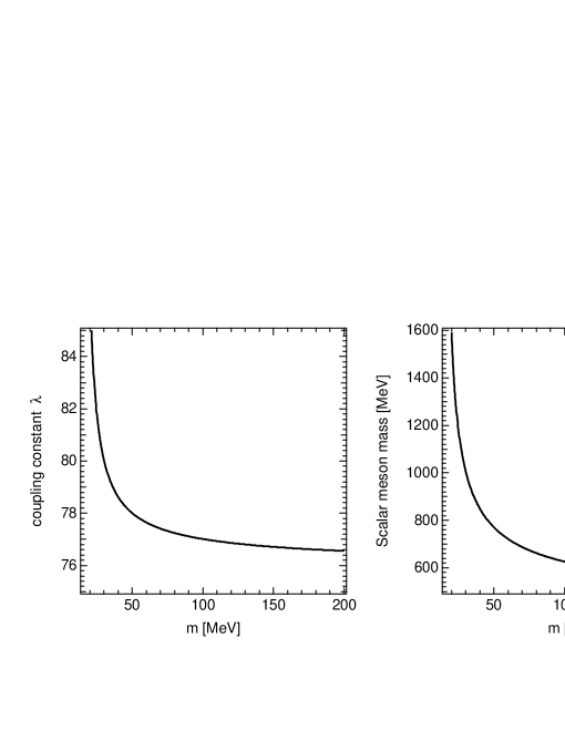
Figure 6: The dependence of the coupling constant $\lambda$ and the mass of the sigma meson on $m$.

We consider here the physical meaning of the renormalization scale $m$ in the massless chiral sigma model through the ratio $\gamma$. At first we consider the coupling constant $\lambda$ (Eq. (36)) and the mass of the sigma meson $m_{\sigma}$ (Eq. (44)) for their dependence on the renormalization scale $m$ in Fig. 6. In the small $m$ region, the dependence of two values on $m$ is large, while it saturates in the large $m$ region. We find an interesting property of dependence on renormalization scale in the limit $m\rightarrow\infty$

$$\lambda \rightarrow 75.315,$$ (52)

$$m_{\sigma} \rightarrow 0.$$ (53)

Especially Eq. (53) shows the restoration of the chiral symmetry in the limit of $m\rightarrow\infty$. Since one-loop corrections give rise to spontaneous chiral symmetry breaking in our model, it means that this generator vanishes in the limit $m\rightarrow\infty$. In order to check this fact we estimate the ratio (Eq. (30)) with Eq. (36),

$$\gamma\rightarrow 1\ \ (m\rightarrow\infty).$$ (54)

As shown in Fig. 7, all of the radiative corrections are perfectly cancelled in this limit, and the mechanism of spontaneous symmetry breaking does not occur. Thus both nucleon and boson becomes massless particle in this phase. Once a renormalization scale has a finite value, the symmetry between fermion and boson is broken. At the same time, spontaneous symmetry breaking occurs and the masses of both nucleon and bosons are generated dynamically. This means that the MCSM becomes trivial for $m=\infty$, while the system becomes non-trivial at finite $m$. It is now legitimate to set $m=f_{\pi}$, since the renormalization condition is naturally taken at the point where the nucleon and all the bosons should have the known physical values in the non-trivial vacuum.

Figure 7: The dependence of the ratio $\gamma$ on $m$. This figure shows that the contribution from the boson loop is larger than the one from the nucleon loop. It corresponds to the result of Fig. 4. Taking the limit $m\rightarrow\infty$ with Eq. (36), this ratio goes to 1. It means that the one-loop corrections from boson and nucleon perfectly cancel each other in this limit.

VI Conclusion

We have studied the vacuum polarization of the Dirac sea with chiral symmetry using the Coleman-Weinberg renormalization procedure. In the Coleman-Weinberg scheme, we start with the massless fermion and boson Lagrangian with the chiral symmetry, where the renormalization scale is chosen at finite $m$. We work out the renormalization procedure and obtain a divergence-free chiral Lagrangian, which includes the vacuum polarization effect. The mean field approximation provides the lowest energy state as the ground state, which corresponds to the sigma field $\phi=f_{\pi}$. We take the renormalization scale at $m=f_{\pi}$, because this is the vacuum state, where the nucleon mass and meson masses are known as the experimental values. Hence, all the parameters in the Lagrangian are fixed by the experiment.

It is interesting to analyze the Coleman-Weinberg renormalization scheme applied to the fermion-boson system with chiral symmetry. The contributions of the loop diagrams of both the fermion and boson come out to have the same functional forms except for the coupling constants. The renormalized Lagrangian at some renormalization scale $m$ provides non-trivial solution with the lowest mean field energy at $\phi=f_{\pi}$ for the case of the finite renormalization scale. However, as $m\rightarrow\infty$ the fermion loop and the boson loop cancel completely each other and the model becomes trivial. In this limit the quantum corrections completely disappears.

We have now a theoretical model to handle the chirally symmetric Lagrangian with the vacuum polarization effect having been worked out. We are now armed to describe the nuclear system at finite nucleon density and also the hadronic system at finite temperature with the model Lagrangian with chiral symmetry.

References

• (1) J. D. Walecka, Ann. of Phys. 83, 491 (1974).
• (2) M. G. Meyer, Phys. Rev. 75, 1969 (1949); O. Haxel, J. H. D. Jensen and H. E. Suess, Phys. Rev. 75, 1766 (1949).
• (3) P. G. Reinhard, M. Rufa, J. Maruhn, W. Greiner and J. Friedrich, Z. Phys. A323, 13 (1986).
• (4) Y. Sugahara and H. Toki, Nucl. Phys. A579, 557 (1994).
• (5) G. A. Lalazissis, J. König and P. Ring, Phys. Rev. C55, 540 (1997).
• (6) G. Mao, H. Stöcker and W. Greiner, Int. J. Mod. Phys. E8, 389 (1999).
• (7) T. Nagata, A. Kato and T. Kohmura, Nucl. Phys. A601, 333 (1996).
• (8) M. Gell-mann and M. Levy, Nuovo Cimento 16, 705 (1960).
• (9) J. Boguta, Phys. Lett. B120, 34 (1983).
• (10) Y. Ogawa, H. Toki, S. Tamenaga, H. Shen, A. Hosaka, S. Sugimoto, K .Ikeda, Prog. Theor. Phys. 111, 75 (2004).
• (11) T. Matsui and B. D. Serot, Ann. of Phys. 144, 107 (1982).
• (12) J. Boguta, Nucl. Phys. A501, 637 (1989).
• (13) S. R. Coleman and E. Weinberg, Phys. Rev. D7, 1888 (1973).
• (14) I. J. Aitchison and C. M. Fraser, Phys. Lett. B146, 63 (1984);
C. M. Fraser, Z. Phys. C28, 101 (1985);
R. J. Perry, Phys. Lett. 182, 269 (1986);
R. J. Furnstahl and C. E. Price, Phys. Rev. C41, 1792 (1990).
• (15) A. Haga, S. Tamenaga, H. Toki, Y. Horikawa, Phys. Rev. C70, 064322 (2004).
• (16) R. J. Furnstahl, B. D. Serot, H. -B. Tang, Nucl. Phys. A618, 446 (1997).
• (17) T. D. Lee and G. C. Wick, Phys. Rev. D9, 2291 (1974);
T. D. Lee and M. Margulies, Phys. Rev. D11, 1591 (1975).
• (18) A. D. Jackson, M. Rho, E. Krotscheck, Nucl. Phys. A407, 495 (1983);
E. M. Nyman and M. Rho, Phys. Lett. B60, 134 (1976).
• (19) B. D. Serot and J. D. Walecka, in Advances in Nuclear Physics, ed. J. W. Negele and E .Vogt (Plenum Press, New York, 1986), vol. 16, p.1.
• (20) S. A. Chin, Ann. of Phys. 108, 301 (1977).
• (21) H. Georgi, Adv. Nucl. Phys. 43, 209 (1993);
H. Georgi and A. Manohar, Nucl. Phys. B234, 189 (1984).
• (22) J. L. Friar, D. G. Madland, B. W. Lynn, Phys. Rev. C53, 3085 (1996).