Abstract

We propose a collective model formalism which describes the strong parity shift observed in low-lying spectra of nuclei with octupole deformations together with the fine rotational band structure developed at higher angular momenta. The parity effect is obtained by the Schrödinger equation for oscillations of the reflection asymmetric (octupole) shape between two opposite orientations in an angular momentum dependent double-well potential. The rotational structure is obtained by a collective quadrupole-octupole rotation Hamiltonian. The model scheme reproduces the complicated beat staggering patterns observed in the octupole bands of light actinide nuclei. It explains the angular momentum evolution of octupole spectra as the interplay between the octupole shape oscillation (parity shift) mode and the stable quadrupole-octupole rotation mode.

PACS: 21.60.Ev; 21.10.Re

Keywords: octupole deformation, alternating parity bands, staggering effect

Short title: Parity shift and beat staggering structure …

1 Introduction

The appearance of reflection asymmetric shapes in atomic nuclei is associated in the geometric model framework with the manifestation of octupole degrees of freedom [1]. The specific physical characteristics of systems with reflection asymmetry are related to the violation of the $\mathcal{R}$- symmetry ($\mathcal{R}$ is the operator of a rotation by $\pi$ about an axis rectangular to a symmetry axis of the system) and the $\mathcal{P}$- symmetry [$\mathcal{P}$ is the space inversion (parity) operator]. It is known that while these symmetries are violated separately, the system can be still invariant with respect to the product operator $\mathcal{P}\mathcal{R}$^-1 [1]. Then the spectrum of the system is characterized with the presence of energy bands in which the parity changes alternatively with the angular momentum.

The best examples of such alternating parity bands, called also octupole bands, are known in the region of light actinide nuclei Rn, Ra and Th [2, 3, 4]. Although the general structure of the observed spectra unambiguously indicates the presence of reflection asymmetry, the detailed analysis of experimental data suggests the manifestation of a more complicated collective dynamics. Thus, a strong parity shift effect is observed in the region of low angular momenta $I<7-8$. The negative parity levels appear above the neighboring even levels with energy $E_{1^{-}}>E_{2^{+}}$, $E_{3^{-}}>E_{4^{+}}$, and so on. Near $I\sim 8-10$ the shift effect rapidly decreases and further at higher angular momenta (up to $I\sim 28$) a single collective octupole band with normally ordered levels is formed. In such a way the data suggest a specific evolution of collectivity with angular momentum.

The properties of nuclei with octupole degrees of freedom have been extensively studied within various geometric, algebraic and microscopic model approaches in nuclear structure (for review see [5] and references therein). In particular, the alternating parity bands have been described in several recent works, most of them covering the low and medium angular momenta $I<18-20$ [6, 7, 8] and some of them reaching the higher region of $I\sim 28$ [9]. These works provide specific model explanations of the properties of octupole deformed nuclei. However, the dynamical mechanism which governs the complete angular momentum evolution of octupole collectivity remains to be understood. Still, the considerable change in the structure of the spectrum from the low-spin region ($I<10-12$) to the medium ($I\sim 12-16$) and higher ($I\sim 20-28$) angular momenta needs an explanation. This is quite clear in view of the “beat” odd-even ($\Delta I=1$) staggering patterns observed in the octupole bands of light actinide nuclei [10]. They correspond to a zigzagging behavior of the odd-even energy difference as a discrete function of $I$ with changing amplitude and presence of one or more zero-amplitude points. Another important circumstance that should be taken into account is that the octupole deformation appears as a superposition on the top of the quadrupole deformation [5]. Therefore, one should consider a system with a complicated quadrupole-octupole shape. A prescription for the most general Hamiltonian of the quadrupole-octupole deformed system is given in [11]. It is based on the Pauli quantization procedure applied to a generalized Bohr Hamiltonian, including the octupole degrees of freedom, with a subsequent transformation to the body fixed frame.

Having in mind the above remarks, we suggest that the complete structure of alternating parity bands can be interpreted within the following general framework. In the low-energy region the system can be characterized by oscillations of the octupole shape between two opposite orientations, which we call soft octupole mode, and by simultaneous rotations of the entire quadrupole–octupole shape. The parity shift is then the result of the tunnelling between the two reflection asymmetric shape orientations separated by an angular momentum dependent potential barrier [12]. With the increase of the angular momentum the energy barrier increases and suppresses respectively the tunnelling effect and the shape oscillations. In such a way a stable quadrupole–octupole shape is formed. At the high angular momenta, the parity effect is completely reduced, and there the properties of collective motion can be associated with the rotation of a stable quadrupole–octupole shape [14].

The purpose of the present work is to provide a model formalism capable to describe the strong parity shift in the low-lying spectra together with the fine rotational band structure developed at higher angular momenta. This is achieved by introducing a double-well potential with an angular momentum dependent energy barrier induced by a centrifugal term and by using the Hamiltonian of the point-symmetry based Quadrupole-Octupole Rotation Model (QORM) [14].

In section 2, the formalism of the soft octupole mode is developed and in section 3 the formalism of QORM is discussed. In section 4, results of the application of both schemes, soft octupole mode and QORM, to spectra of several light actinide nuclei are presented. In section 5, concluding remarks are given.

2 Soft octupole deformation and parity shift effect

The model frame for the description of the parity shift effect in nuclei with octupole deformations can be defined through the following main assumptions:

i) The parity shift in octupole bands is determined by the oscillation of the system with respect to a deformation variable $\beta$ in a symmetric double-well potential centered at $\beta=0$. We assume that $\beta$ is related to the axial octupole deformation ($Y_{30}$).

ii) The potential barrier increases with the increase of the angular momentum $I$ as the result of a centrifugal interaction with a deformation dependent moment of inertia.

iii) The octupole deformation $\beta_{\mbox{\scriptsize min}}$ in the minimum of the potential does not change with the angular momentum. Therefore, with increasing $I$ the octupole shape “stabilizes” to a fixed octupole deformation.

iv) The parity shift can be extracted from the potential energy by excluding the contribution of the rotation mode. The rotation degrees of freedom can be considered separately without double counting in the potential energy.

v) For given $I$ the intrinsic state is determined by the lowest level in the potential whose parity $\pi$ together with the $\mathcal{R}$- symmetry of the rotation wave function, $(-1)^{I}$, conserves the total $\mathcal{P}\mathcal{R}$^-1-symmetry, $s=\pi(-1)^{I}$. Thus for $I=$even the intrinsic state of the system is determined by the first level $E_{I}^{(+)}$ in the potential with $\pi=(+)$. For $I=$odd it is determined by the second level $E_{I}^{(-)}$ with $\pi=(-)$.

The Hamiltonian for oscillations in the octupole shape (the soft octupole mode) can be taken in the general form

$$H^{\mbox{\scriptsize oct}}_{\mbox{\scriptsize osc}}=-\frac{\hbar^{2}}{2B_{3}}\frac{d^{2}}{{d\beta}^{2}}+U_{I}(\beta)\ ,$$ (1)

where $B_{3}$ is an effective octupole mass parameter. The potential $U_{I}(\beta)$ is determined as follows. We consider the angular momentum dependent potential

$$U(\beta,I)=\frac{1}{2}C{\beta}^{2}+\frac{1}{2{\mathcal{L}}(\beta)}I(I+1)\ .$$ (2)

The quantity ${\mathcal{L}}(\beta)$ can be associated to the moment of inertia of the system taken in the form ${\mathcal{L}}(\beta)=d_{1}+d_{2}\beta^{2}$, where $d_{1},\,d_{2}>0$ are constants. Such a dependence can be explained through the moment of inertia of an axial symmetric quadrupole-octupole shape, ${\mathcal{L}}^{(\mbox{\scriptsize quad+oct})}\sim 3B_{2}\beta^{2}_{\mbox{\scriptsize quad}}+6B_{3}\beta^{2}_{\mbox{\scriptsize oct}}$, where $\beta_{\mbox{\scriptsize quad}}$ and $\beta_{\mbox{\scriptsize oct}}=\beta$ are the quadrupole and octupole deformation parameters, respectively [15]. For a stable quadrupole deformation, $\beta_{\mbox{\scriptsize quad}}=\mbox{const}$, ${\mathcal{L}}^{(\mbox{\scriptsize quad+oct})}$ reduces to the above form of ${\mathcal{L}}(\beta)$, and the potential (2) reads

$$U(\beta,I)=\frac{1}{2}C{\beta}^{2}+\frac{X(I)}{d_{1}+d_{2}\beta^{2}}\ ,$$ (3)

with $X(I)=I(I+1)/2$. For $X(I)/C>d_{1}^{2}/2d_{2}$, the shape of the potential (3) represents a double well with a potential barrier centered at $\beta=0$. The term quadratic in $\beta$ generates oscillations of the reflection asymmetric (octupole) shape between two opposite orientations of the system, providing a parity shift effect in the collective energy. The second term in (3) corresponds to a centrifugal interaction generating a potential barrier. The height of the barrier increases with increasing $I$ and suppresses respectively the parity shift.

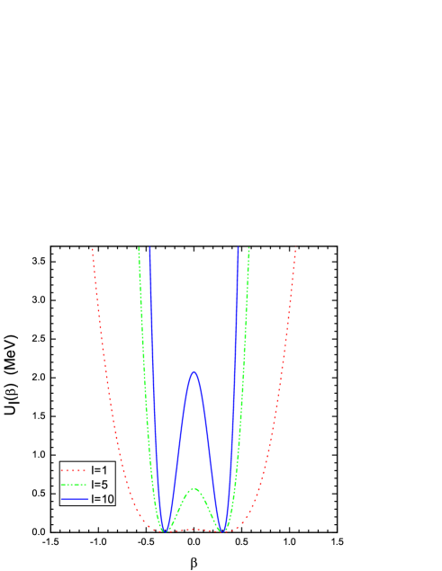
Figure 1: The octupole deformation potential (6) is plotted for three different values of the angular momentum $I=1,5,10$. The parameters values used in equation (6) are given in figure 2.

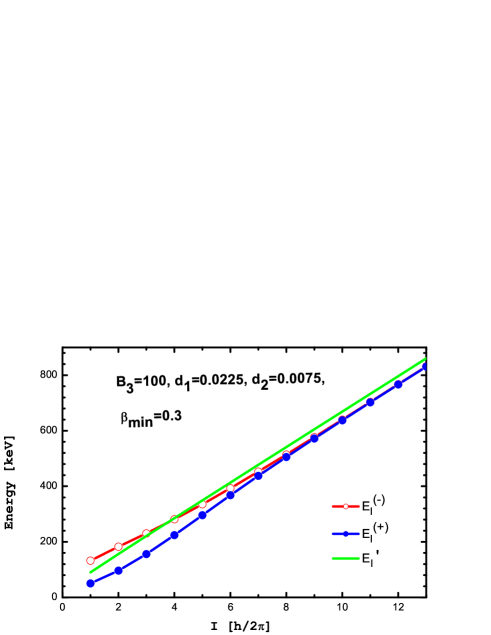
Figure 2: The first and the second energy levels $E_{I}^{(+)}$ and $E_{I}^{(-)}$ in the potential (6) as well as the approximating oscillator energy $E^{\prime}_{I}$, equation (7), are shown as functions of angular momentum. The parameters $B_{3}$, $d_{1}$ and $d_{2}$ are given in $\hbar^{2}$/MeV, MeV^-1 and MeV^-1, respectively, while $\beta_{\mbox{\scriptsize min}}$ is dimensionless.

We remark that double-well potentials without angular momentum dependence of the potential barrier have been considered in earlier works [16, 17]. Some general properties of angular momentum dependent double-well potentials have been discussed in references [12, 13]. A spin-dependent potential with a centrifugal term similar to that in (3) has been applied in [18, 19] in reference to the phase transitions in nuclei with octupole degrees of freedom.

Following the assumption iii), we consider that the potential $U(\beta,I)$ has a minimum at some fixed value of $\beta=\beta_{\mbox{\scriptsize min}}$. The extremum condition $\left.\frac{\partial}{\partial\beta}U(\beta,I)\right|_{\beta_{\mbox{\scriptsize min}}}=0$ gives

$$C\equiv C(I)=\frac{2X(I)d_{2}}{(d_{1}+d_{2}\beta_{min}^{2})^{2}}.$$ (4)

Thus, the requirement for a fixed potential minimum in the octupole deformation imposes an angular momentum dependence of the parameter $C$. The substitution of equation (4) into (3), leads to the following form of the octupole potential

$$U(\beta,I)=\frac{X(I)}{d_{1}+d_{2}\beta^{2}}\left[1+\frac{d_{2}(d_{1}+d_{2}\beta^{2})}{(d_{1}+d_{2}\beta_{\mbox{\scriptsize min}}^{2})^{2}}\beta^{2}\right]\ .$$ (5)

To eliminate (according to assumption iv) the angular momentum (rotation) dependence of the origin of the energy scale we determine the potential as $U_{I}(\beta)=U(\beta,I)-U(\beta_{\mbox{\scriptsize min}},I)$,

$$U_{I}(\beta)=\frac{X(I)d_{2}^{2}(\beta^{2}-\beta_{\mbox{\scriptsize min}}^{2})^{2}}{(d_{1}+d_{2}\beta_{\mbox{\scriptsize min}}^{2})^{2}(d_{1}+d_{2}\beta^{2})}.$$ (6)

The evolution of the potential (6) with the angular momentum is demonstrated in figure 1. It is seen that, the increase in the potential barrier with $I$ is associated with a respective decrease in the width of the potential well. This corresponds to an increasing stiffness of the system, and therefore, to a rapid stabilization of the shape in the higher angular momenta.

Figure 3: Numerical behavior of the octupole oscillation term $E_{\mbox{\scriptsize osc}}(I)$ (8) [part (a)] and its contribution to the staggering quantity (9) [part (b)]. $E_{0}$ is given in keV, while the other parameters are as in figure 2.

We determine the energy levels $E_{I}^{(+)}$ and $E_{I}^{(-)}$ [according to the assumption v)] in the potential $U_{I}(\beta)$ [equation (6)] by solving numerically the Schrödinger equation with the Hamiltonian (1). These energies still carry a rotation input due to the narrowing of the potential minima. As shown in figure 2, the both levels increase with $I$. To estimate analytically this dependence we approximate the shapes of the potential minima by $U^{\prime}_{I}(\beta)=(1/2)C^{\prime}(I)(|\beta|-\beta_{\mbox{\scriptsize min}})^{2}$, with $C^{\prime}(I)=\left.\frac{\partial^{2}}{\partial\beta^{2}}U_{I}(\beta)\right|_{\beta_{\mbox{\scriptsize min}}}$. The lowest energy level in this potential is

$$E^{\prime}_{I}=\frac{\hbar}{2}\sqrt{\frac{C^{\prime}(I)}{B_{3}}}=\frac{\hbar}{\sqrt{2B_{3}}}\frac{d_{2}\beta_{\mbox{\scriptsize min}}}{(d_{1}+d_{2}\beta_{\mbox{\scriptsize min}}^{2})^{3/2}}\sqrt{I(I+1)}.$$ (7)

It approximates the overall increase of the levels $E_{I}^{(+)}$ and $E_{I}^{(-)}$ as demonstrated in figure 2. Thus, to keep only the parity dependence in the intrinsic energy according to assumption iv), and not the part nearly linearly increasing with $I$ one should set the energy of the octupole shape oscillations in the form

$$E_{\mbox{\scriptsize osc}}(I)=E_{0}-\frac{1}{2}(-1)^{I}\delta E(I),$$ (8)

where $\delta E(I)=E_{I}^{(-)}-E_{I}^{(+)}$ and $E_{0}$ is a constant. Thus the intrinsic energy related to octupole degrees of freedom is separated in a part independent of the angular momentum, and an “alternating” part, which takes into account the shift down (for $I=$even) and the shift up (for $I=$odd) of the intrinsic “octupole” energy with respect to $E_{0}$. So, equation (8) approximates the non-rotational part of the energy in the alternating parity bands.

The angular momentum dependence of $E_{\mbox{\scriptsize osc}}(I)$ is demonstrated in figure 3(a). We see that in the low spin region it exhibits a strongly oscillating behavior. With increasing $I$ the oscillations rapidly vanish and $E_{\mbox{\scriptsize osc}}(I)$ is reduced to the constant $E_{0}$. In figure 3(b) we illustrate the contribution of $E_{\mbox{\scriptsize osc}}(I)$ to the higher order staggering quantity

$$\mbox{Stg}(I)=6\Delta E(I)-4\Delta E(I-1)-4\Delta E(I+1)+\Delta E(I+2)+\Delta E(I-2)\ ,$$ (9)

where $\Delta E(I)=E(I+1)-E(I)$. As it is seen from figure 3(b), for $E(I)\equiv E_{\mbox{\scriptsize osc}}(I)$, this quantity shows a well developed staggering pattern with a rapidly decreasing magnitude similar to what is observed in the low spin region of alternating parity bands in light actinide nuclei [10]. However, while the solutions of the Schrödinger equation for the Hamiltonian (1) suggest a complete disappearance of the parity shift and the respective staggering after some point, the experimental data show [10] more complicated “beat” patterns with the presence of further staggering regions at higher angular momenta. This additional staggering regions can not be explained by the octupole oscillation mode. Their presence can be attributed to the properties of a rotating system with a stable quadrupole-octupole deformation which will be considered in the next section.

3 The Quadrupole–Octupole Rotation Model

The Quadrupole–Octupole Rotation Model (QORM) has been proposed for the description of rotation motion in nuclear systems in the presence of stable quadrupole–octupole shapes [14]. The general model Hamiltonian is given in the form

$$\hat{H}_{\mbox{\scriptsize QORM}}=\hat{H}_{\mbox{\scriptsize quad}}+\hat{H}_{\mbox{\scriptsize oct}}+\hat{H}_{\mbox{\scriptsize qoc}}\ .$$ (10)

The quadrupole rotation term

$$\hat{H}_{\mbox{\scriptsize quad}}=A\hat{I}^{2}+A^{\prime}\hat{I}_{z}^{2}$$ (11)

provides the general energy scale for rotation motion of the nucleus. The octupole Hamiltonian part

$$\hat{H}_{\mbox{\scriptsize oct}}=\hat{H}_{A_{2}}+\sum_{r=1}^{2}\sum_{i=1}^{3}\hat{H}_{F_{r}(i)}$$ (12)

is constructed by using the irreducible representations $A_{2}$, $F_{1}(i)$ and $F_{2}(i)$ ($i=1$, 2, 3) of the octahedron $(O)$ point–symmetry group, where

$$\hat{H}_{A_{2}}={a}_{2}\frac{1}{4}[(\hat{I}_{x}\hat{I}_{y}+\hat{I}_{y}\hat{I}_{x})\hat{I}_{z}+\hat{I}_{z}(\hat{I}_{x}\hat{I}_{y}+\hat{I}_{y}\hat{I}_{x})]\ ,$$ (13)

$$\hat{H}_{F_{1}(1)}=\frac{1}{2}{f}_{11}(5\hat{I}_{z}^{3}-3\hat{I}_{z}\hat{I}^{2}) \hat{H}_{F_{2}(1)}={f}_{21}\frac{1}{2}[\hat{I}_{z}(\hat{I}_{x}^{2}-\hat{I}_{y}^{2})+(\hat{I}_{x}^{2}-\hat{I}_{y}^{2})\hat{I}_{z}]$$

$$\hat{H}_{F_{1}(2)}=\frac{1}{2}{f}_{12}(5\hat{I}_{x}^{3}-3\hat{I}_{x}\hat{I}^{2}) \hat{H}_{F_{2}(2)}={f}_{22}(\hat{I}_{x}\hat{I}^{2}-\hat{I}_{x}^{3}-\hat{I}_{x}\hat{I}_{z}^{2}-\hat{I}_{z}^{2}\hat{I}_{x})$$ (14)

$$\hat{H}_{F_{1}(3)}=\frac{1}{2}{f}_{13}(5\hat{I}_{y}^{3}-3\hat{I}_{y}\hat{I}^{2}) \hat{H}_{F_{2}(3)}={f}_{23}(\hat{I}_{y}\hat{I}_{z}^{2}+\hat{I}_{z}^{2}\hat{I}_{y}+\hat{I}_{y}^{3}-\hat{I}_{y}\hat{I}^{2})\ .$$

The different terms in $\hat{H}_{\mbox{\scriptsize oct}}$ (cubic combinations of angular momentum operators in the body fixed frame) represent the contribution of the various octupole shapes to the rotation energy with a magnitude determined by the parameters ${a}_{2}$ and ${f}_{r\,i}$ ($r=1,2;\,i=1,2,3$). The last term in equation (10) represents a higher order quadrupole–octupole interaction [14]

$$\hat{H}_{\mbox{\scriptsize qoc}}=f_{\mbox{\scriptsize qoc}}\frac{1}{I^{2}}(15\hat{I}_{z}^{5}-14\hat{I}_{z}^{3}\hat{I}^{2}+3\hat{I}_{z}\hat{I}^{4}).$$ (15)

The energy corresponding to the diagonal part of $\hat{H}_{\mbox{\scriptsize QORM}}$ in the states $|IK\rangle$ with collective angular momentum $I$ and intrinsic projection $K$ has the form

$$E_{K}(I) = AI(I+1)+A^{\prime}K^{2}+\frac{1}{2}f_{11}\left(5K^{3}-3KI(I+1)\right)$$ (16)

$$+ f_{\mbox{\scriptsize qoc}}\frac{1}{I^{2}}\left(15K^{5}-14K^{3}I(I+1)+3KI^{2}(I+1)^{2}\right)\ .$$

We remark that a similar structure of the high order angular momentum terms can be obtained by applying the method of contact transformations [1, 20] to a Hamiltonian including the intrinsic particle motion and the Coriolis interaction [21]. The analysis in reference [21] provides a deeper physical meaning of the QORM Hamiltonian parameters in relation to the matrix elements of the intrinsic angular momentum operators in the intrinsic single particle states.

Equation (16) provides the main part of the collective rotation energy corresponding to the QORM Hamiltonian. The off-diagonal terms in the octupole Hamiltonian (12) [see equations. (14)] have to be taken into account through a numerical diagonalization procedure. Since the octupole shape is fixed with respect to the space orientation angles, only three off-diagonal terms, $\hat{H}_{F_{1}(2)}$, $\hat{H}_{F_{2}(1)}$ and $\hat{H}_{F_{2}(2)}$ are considered to contribute to the structure of the spectrum [14]. Further, one may keep only terms mixing states with neighboring $K$ values, i.e. $K\pm 1$, omitting the term $\hat{H}_{F_{2}(1)}$ (with $K\pm 2$ mixing) whose contribution is essentially smaller. Then, noticing that the matrix elements of the remaining terms $\hat{H}_{F_{1}(2)}$ and $\hat{H}_{F_{2}(2)}$ have similar angular momentum dependences (see the appendix in reference [14]) we realize that the use of any one of them could provide a reasonable non-diagonal octupole contribution to the energy of the system.

The model spectrum is obtained by minimizing the energy in the diagonal part of $\hat{H}_{\mbox{\scriptsize QORM}}$, equation (16), with respect to $K$ and by diagonalizing the total Hamiltonian (with the appropriate non-diagonal terms) in the set of states $|IK\rangle$. The energy-minimum values of the quantum number $K$, resulting from the minimization procedure, gradually increase with the increase of $I$, forming a sequence of the type $K=0,0,1,1,2,2,...$ for $I=1,2,3,4,5,6,...$. The increase of $K$ after two consecutive equal values by a unit (a discrete jump) generates an odd-even ($\Delta I=1$) staggering effect in the collective band structure. The regularity of the $K$- sequence depends on the behavior of the energy (16) as a function of $K$ and of the respective change of its minimum with $I$ (see figure 4). The numerical analysis of this behavior shows that after a range of regularly ordered sequence, at some value of $I$ there is an appearance of a single $K$- value $K=K_{s}$. For example one may have $K=...,K_{s}-1,K_{s}-1,K_{s},K_{s}+1,K_{s}+1,...$ The presence of such an irregularity in the sequence causes an irregularity in the $\Delta I=1$ staggering pattern. As a result the phase of the oscillations is changed [the sign of the staggering quantity (9) is inverted] and a “beat” staggering region is formed. The angular momentum values where such irregularities appear depend on the model parameters entering the energy expression (16). A detailed justification and specific tests related to the appearing yrast $K$- sequences are given in sec. VI of reference [14].

In such a way the QORM Hamiltonian explains the appearance of “beats” in the staggering patterns of nuclear octupole bands. It has been demonstrated that QORM is capable to reproduce the “beat” staggering effects in the high angular momentum regions of alternating parity spectra in light actinide nuclei [22, 23]. We should remark that the above presented formalism can not describe alone the lowest levels of alternating parity bands where the soft (oscillating) octupole mode dominates the odd-even angular momentum shift.

4 Description of the complete alternating parity band structure

The application of the formalism of the “soft” octupole mode (given in section 2) and the model Hamiltonian of QORM (section 3) allows us to describe the complete structure of nuclear alternating parity bands. We take the collective model energy of the quadrupole–octupole deformed system in the form

$$E_{\mbox{\scriptsize coll}}(I)=E_{\mbox{\scriptsize osc}}(I)+E_{\mbox{\scriptsize QORM}}(I)\ ,$$ (17)

where $E_{\mbox{\scriptsize osc}}(I)$, is given in equation (8) and determined through the numerical solution of the Schrödinger equation for the potential (6) as explained in section 2. It depends on the constant $E_{0}$, the deformation $\beta_{\mbox{\scriptsize min}}$ in the potential minimum, and the inertial parameters $d_{1}$ and $d_{2}$ of the centrifugal term in equation (3). We take the same value for the mass parameter $B_{3}=200$ $\hbar^{2}$/MeV in all nuclei under study, as done in [13]. The second term in equation (17), $E_{\mbox{\scriptsize QORM}}(I)$, represents the rotation energy of the quadrupole–octupole shape determined by $\hat{H}_{\mbox{\scriptsize QORM}}$, equation (10), within the procedure explained in the end of section 3 and presented in more details in [14]. Here we consider that $E_{\mbox{\scriptsize QORM}}(I)$ depends on the quadrupole parameters $A$ and $A^{\prime}$, the octupole shape parameters $f_{11}$ and $f_{12}$ [see equation (16) and equations (14)], and the parameter of quadrupole–octupole interaction, $f_{\mbox{\scriptsize qoc}}$, equation (15).

Table 1: Theoretical and experimental energy levels (in keV) of the octupole bands in ²²⁴Ra, ²²⁶Ra, ²²⁴Th and ²²⁶Th. The respective parameter values are given in figures 4-7. References for the experimental data are given in the respective columns. The RMS deviations (in keV) are given at the bottom.

	224Ra		226Ra		224Th		226Th
$I$	th	exp [2]	th	exp [2]	th	exp [3]	th	exp [4]
1	245.6	215.9	281.8	253.7	241.4	251.0	215.2	230.4
2	99.1	84.5	63.2	67.7	110.2	98.1	105.2	72.2
3	298.6	290.5	352.4	321.5	327.0	305.3	312.6	307.5
4	276.3	251.0	210.7	211.7	294.4	284.1	237.4	226.4
5	415.8	433.1	441.7	447.0	466.5	464.5	454.6	450.5
6	490.6	479.6	421.5	416.7	540.3	534.7	445.1	447.3
7	619.4	641.0	599.6	627.2	692.9	699.5	654.8	657.9
8	743.7	755.7	668.1	669.6	829.2	833.9	715.3	721.9
9	888.3	906.9	828.2	858.2	991.2	997.7	914.2	923.1
10	1043.5	1069.4	947.5	960.3	1163.7	1173.8	1032.3	1040.3
11	1207.9	1221.7	1108.9	1133.5	1343.9	1347.3	1227.5	1238.4
12	1387.9	1414.7	1262.7	1281.6	1541.2	1549.8	1388.6	1395.2
13	1570.0	1578.3	1434.5	1448.0	1739.2	1738.7	1588.2	1596.0
14	1771.5	1788.5	1612.7	1628.9	1955.2	1958.9	1778.7	1781.5
15	1968.1	1969.4	1796.2	1796.5	2167.8	2164.7	1987.0	1989.4
16	2183.2	2188.7	1993.8	1998.7	2397.9	2398.0	2197.0	2195.8
17	2396.0	2388.8	2187.4	2174.9	2621.1	2620.2	2414.9	2412.8
18	2621.2	2613.1	2400.0	2389.8	2861.0	2864.0	2637.6	2635.1
19	2847.3	2831.7	2602.1	2579.3			2863.8	2861.1
20	3079.3	3060.2	2821.8	2801.1			3094.0	3097.1
21	3316.0	3294.5	3034.7	3006.7
22	3551.3	3527.3	3258.3	3232.7
23	3795.9	3774.3	3479.6	3454.9
24	4031.0	4012.4	3704.2	3685.6
25	4280.6	4271.1	3931.2	3921.9
26	4512.1	4513.2	4153.9	4158.2
27	4760.6	4782.7	4384.0	4405.9
28	4988.6	5031.4	4601.8	4650.7
RMS	$19.0$		$20.4$		$8.1$		$9.8$

We have applied the above presented formalism to the alternating parity bands of the nuclei ^224,226Ra and ^224,226Th. We choose them as the best examples for nuclear spectra carrying both octupole deformation characteristics and pronounced collective rotation structure. In addition the spectra in ^224,226Ra are characterized with well developed beat staggering patterns. After adjusting the model parameters to the respective experimental data, we have obtained a good agreement between the theoretical and experimental levels with a standard root mean square (RMS) deviation of 19 keV for ²²⁴Ra, 20.4 keV for ²²⁶Ra, 8.1 keV for ²²⁴Th and 9.8 keV for ²²⁶Th. This is shown in table 1, where the theoretical and experimental energy values are compared. The respective $\Delta I=1$ staggering patterns have been also reproduced successfully. The theoretical and experimental staggering patterns are compared in figures 4-7. The theoretical patterns are extended providing model prediction for the structure of octupole bands above the experimentally observed angular momenta.

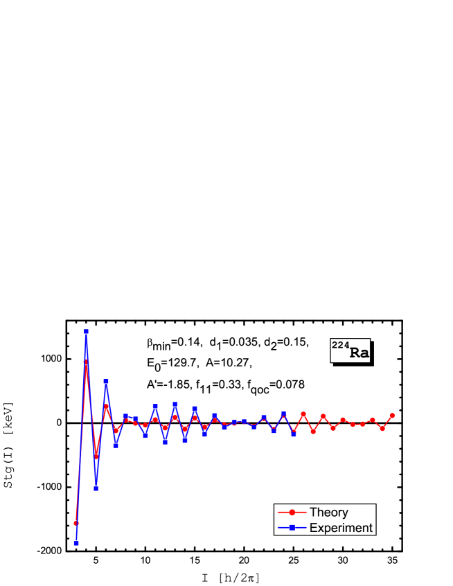
Figure 4: $\Delta I=1$ staggering patterns for the octupole band in ²²⁴Ra: experiment (data from [2]) and theory. The parameters $B_{3}$, $d_{1}$ and $d_{2}$ are given in $\hbar^{2}$/MeV, MeV^-1 and MeV^-1, respectively, $\beta_{\mbox{\scriptsize min}}$ is dimensionless, while the other parameters are in keV.

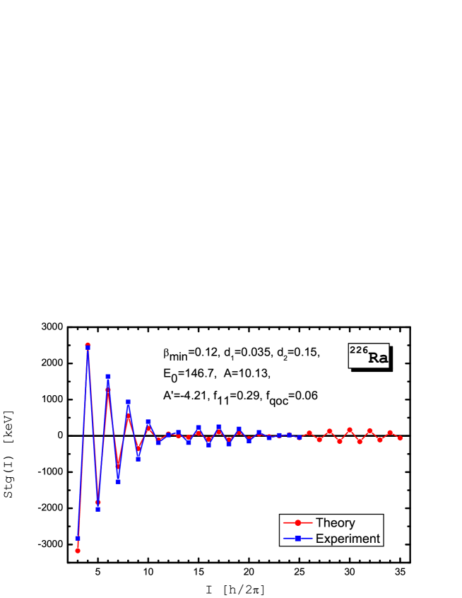
Figure 5: The same as in figure 4, but for the octupole band of ²²⁶Ra.

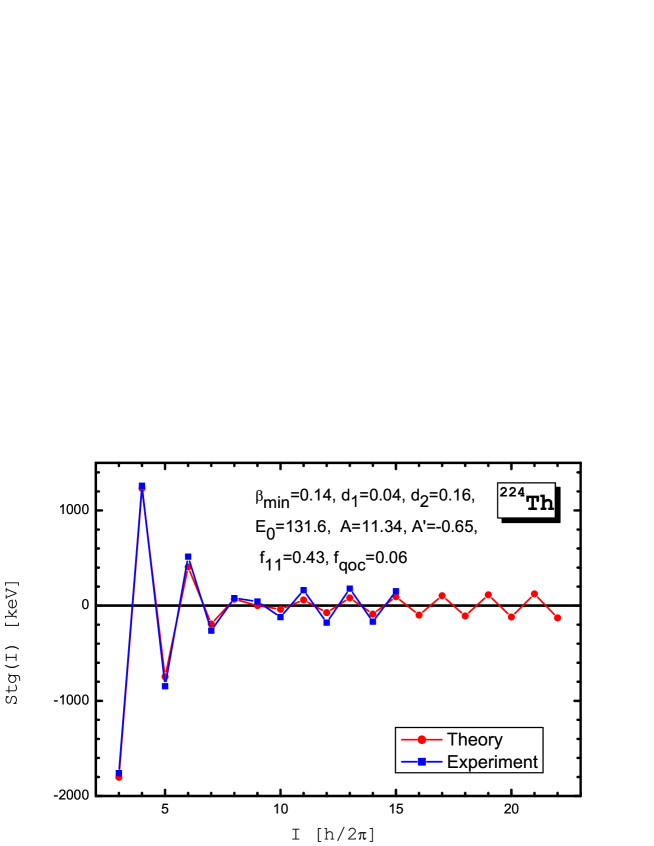
Figure 6: The same as in figure 4, but for the octupole band of ²²⁴Th. Data from [3].

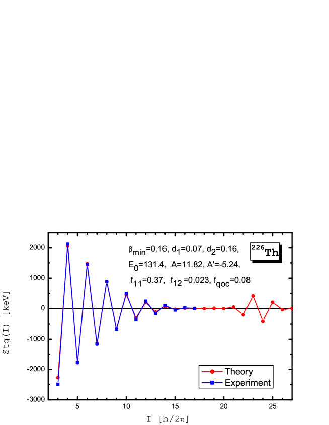
Figure 7: The same as in figure 4, but for the octupole band of ²²⁶Th. Data from [4].

The following comments on the obtained results have to be made.

i) The model description reproduces correctly the points with near zero staggering amplitude, which separate the different beat regions in the staggering patterns. In this way the model formalism clearly identifies the angular momentum region where the two separate sequences of negative and positive parity levels merge into a single octupole rotational band. We note that both modes, the soft octupole and the stable quadrupole–octupole, fit to each other quite consistently.

ii) As a consequence of i), our results show that the complicated odd-even staggering structure of alternating parity bands can be explained as the result of two consistently manifesting dynamical effects in the nucleus. The one is the parity splitting effect due to oscillations in the orientation (tunnelling effect) of the octupole shape and the other is the ”beat” staggering effect due to the angular momentum properties (with the specific sequences of $K$-values described in the end of section 3) of the rotating quadrupole–octupole shape. So, our model description suggests that in the low angular momentum region of the spectrum the staggering effect is mainly due to the parity effect, while in the higher spin region the beat staggering structure of the band is due to the rotating complex shape. In this aspect the first “zero” in the staggering amplitude can be attributed to a transition angular momentum region where the nuclear collectivity changes from the soft octupole to the stable rotation behavior.

iii) The successful reproduction of the second and the third beat regions in the staggering patterns of ²²⁴Ra and ²²⁶Ra provides a useful theoretical tool for the analysis and prediction of collective band structure at high angular momenta. This is a result of the model mechanism presented in the end of section 3. According to the explanation given there, the presence of second, third and further “zeros” in the staggering amplitude can be interpreted as the result of respective irregularities in the yrast $K$-sequences. Our calculations predict that the third staggering region in ²²⁴Ra (figure 4) could be completed near $I=30$ and a fourth region could be expected if further experimental data are obtained. In ²²⁶Ra (figure 5), again an additional third beat is expected near $I=30$. In ²²⁴Th (figure 6) the prediction suggests that the second staggering region could be continued in the region $I=15-20$, while in ²²⁶Th (figure 7) the expectation is that a second staggering region can take place for $I>20$. So, any further experimental data in these spectra will be of great interest to test the model predictions.

iv) We remark that the current calculations predict the presence of a non-axial octupole deformation in ²²⁶Th with an off-diagonal parameter value $f_{12}=0.023keV$. For the other considered nuclei $f_{12}$ obtains zero values. The appearance of a non-zero value of $f_{12}$ can be related to the recently suggested shape phase transition between the regions of octupole deformations and octupole vibrations [24]. It was shown that the nuclei ²²⁶Ra and ²²⁶Th are closely placed to the transition point. In this meaning the presence of triaxiality could be interpreted as the sign of the transition from octupole deformation to octupole vibration.

The following comments on the applied model approach and its further development should take a place here.

i) Although the total number of used model parameters looks large, their numerical values in the different nuclei vary in quite narrow limits (See the values shown in figures 4-7). We could keep some of them ($d_{1}$ or $d_{2}$, $A$ and $A^{\prime}$) as overall constants similarly to the mass parameter $B_{3}$, without essential loss of accuracy. However, at the current stage of study we prefer to consider them as the output of the fitting procedure because of their clear physical meaning. This consideration holds especially for the parameter $\beta_{\mbox{\scriptsize min}}$ which provides a direct model prediction for the octupole deformations of nuclei. Actually it could be related to the QORM Hamiltonian parameter $f_{11}$ through the nuclear moment of inertia. As a consequence a possible change in $\beta_{\mbox{\scriptsize min}}$ with increasing angular momentum could be allowed. Such a consideration would be a step towards constructing a single model Hamiltonian where the same degrees of freedom are incorporated and which possesses two different limiting cases for low and high angular momenta.

ii) We note that further refinements of the considered approach are possible. For example, it is known that the experimentally observed parity shift in the light actinide nuclei decreases with the angular momentum almost exponentially [13]. We see in figure 3(a) that in the first few levels with $I=1,2,3$ the theoretical splitting does not decrease enough rapidly to fit this exponential behavior, while for $I>3$ the fast decrease is already reached. We notice that the behavior of the theoretical splitting for $I<3$ is due to the change of the potential shape from a parabola at $I=0$ to the double–well for $I>0$, which affects most strongly the energy shift in $I=1$ and $I=2$. As a result relatively large discrepancies between the theoretical and experimental energy values are observed at these angular momenta (see table 1), with the related $R_{4}=E(L=4)/E(L=2)$ ratios (characteristics of collectivity) being also affected. This problem can be fixed if the potential (3) is modified so as to obtain a double–well shape at $I=0$. The modification can be achieved by applying in equation (3) the term $d_{0}+X(I)$ instead of $X(I)$, where $d_{0}$ is a constant. A numerical analysis shows that the behavior of the theoretical parity splitting and the respective values of the low energy levels can be better reproduced by means of the additional parameter $d_{0}$. So we suggest that such efforts should be done in a further work after the electromagnetic transition probabilities being considered (see below).

iii) The present formalism is capable of providing model predictions on $B(E1)$, $B(E2)$ and $B(E3)$ reduced transition probabilities between levels of alternating parity bands. Their specific model behavior is related to the changing values of $K$ in the collective angular momentum states $|IK\rangle$. Our preliminary analysis indicates that specific staggering effects in the transition probabilities could be expected on this basis. On the other hand the presence of $K$- mixing amplitudes coming from the non-diagonal terms in the QORM Hamiltonian would restrict such a staggering behavior. Therefore, the involvement of electromagnetic transition probabilities in the study would make the model more sensitive to the presence of non-axial octupole deformations. In addition, the involvement of the “intrinsic” wave function determined in the solution of the Schrödinger equation is of importance in the model analysis of electromagnetic transition probabilities. This study is the subject of further work.

5 Summary

In conclusion, we propose a collective model formalism incorporating the characteristics of the soft (oscillating) octupole mode and the properties of the stable quadrupole–octupole shapes in nuclei. This formalism is capable to reproduce the entire structure of nuclear alternating parity bands. We showed that it provides a successful description of the octupole bands and their staggering structure in several light actinide nuclei. The complicated “beat” staggering patterns are explained as the result of the interplay between octupole shape oscillations in a spin-dependent double-well potential and rotations of the quadrupole–octupole shape. The model analysis clearly indicates the transition between these two collective modes. So, the implemented study suggests a specific dynamical mechanism for the evolution of quadrupole–octupole collectivity. The model predictions outline a possible way for development of collectivity in the higher angular momenta with a presence of further staggering regions. The considered dynamical mechanism can govern a wide range of properties of nuclei with complex shapes.

Acknowledgements

We thank Professor R V Jolos for valuable discussions and advises. This work is supported by DFG and by the Bulgarian Scientific Fund under contract No F-1502/05.

References

- [1] Bohr A and Mottelson B R 1975 Nuclear Structure, vol. II (New York: Benjamin)
- [2] Cocks J F C et al 1997 Phys. Rev. Lett. 78 2920
- [3] Artna-Cohen A 1997 Nucl. Data Sheets 80 227
- [4] Akovali Y A 1996 Nucl. Data Sheets 77 433
- [5] Butler P A and Nazarewicz W 1996 Rev. Mod. Phys. 68 349
- [6] Denisov V Yu, Dzyublik A Ya 1995 Nucl. Phys. A 589 17
- [7] Zamfir N V and Kusnezov D 2001 Phys. Rev. C 63 054306
- [8] Shneidman T M, Adamian G G, Antonenko N V, Jolos R V and Scheid W 2002 Phys. Lett. B 526 322; 2003 Phys. Rev. C 67 014313
- [9] Raduta A A and Ionescu D, Ursu I I and Faessler A 2003 Nucl. Phys. A 720 43
- [10] Bonatsos D, Daskaloyannis C, Drenska S, Karoussos N, Minkov N, Raychev P and Roussev R 2000 Phys. Rev. C 62 024301
- [11] Rohoziński S G, Gajda M and Greiner W 1982 J.Phys. G 8 787
- [12] Jolos R, Brentano P von and Dönau F 1993 J. Phys. G 19 L151
- [13] Jolos R, Brentano P von 1994 Phys. Rev. C 49 R2301
- [14] Minkov N, Drenska S, Raychev P, Roussev R and Bonatsos D 2001 Phys. Rev. C 63 044305
- [15] Davidson J P 1968 Collective Models of the Nucleus (New York and London: Academic Press)
- [16] Krappe H J and Wille U 1969 Nucl. Phys. A 124 641
- [17] Leander G A, Sheline R K, Möller P, Olanders P, Ragnarsson I and Sierk A J 1982 Nucl. Phys. A 388 452
- [18] Bizzeti P G 2003 in Symmetries in Nuclear Physics, ed Vitturi A and Casten R F (World Scientific, Singapore) p.262; Bizzeti P G and Bizzeti-Sona A M 2004 Eur. Phys. J. A 20 179
- [19] Bizzeti P G and Bizzeti-Sona A M 2004 Phys. Rev. C 70 064319
- [20] Birss F W and Choi J H 1970 Phys. Rev. A 2 1228
- [21] Jolos R V, Minkov N and Scheid W 2005 Phys. Rev. C, 72 064312
- [22] Minkov N and Drenska S 2002 Prog. Theor. Phys. Suppl. 146 597
- [23] Minkov N, Drenska S and Yotov P 2002 in Proceedings of the 21-st International Workshop on Nuclear Theory (Rila, Bulgaria 2002), ed. V. Nikolaev, (Heron Press, Sofia) p. 290
- [24] Bonatsos D, Lenis D, Minkov N, Petrellis D and Yotov P 2005 Phys. Rev. C 71 064309