The nucleon-sigma coupling constant in QCD Sum Rules

Abstract

The external-field QCD Sum Rules method is used to evaluate the coupling constant of the light isoscalar-scalar meson (“$\sigma$” or $\varepsilon$) to the nucleon. The contributions that come from the excited nucleon states and the response of the continuum threshold to the external field are calculated. The obtained value of the coupling constant is compatible with the large value required in one-boson exchange potential models of the two-nucleon interaction.

I Introduction

The values of the meson-baryon coupling constants are of particular interest in understanding the nucleon-nucleon (NN) Nag78 ; Sto94 and hyperon-nucleon (YN) Mae89 ; Rij98 interactions in terms of e.g. one-boson exchange (OBE) models. The scalar mesons play a significant role in such phenomenological potential models. The structure and even the status of the scalar mesons have, however, always been controversial Tim94 ; Swa94 . In early OBE models for the NN interaction the exchange of an isoscalar-scalar “$\sigma$” meson with a mass of about 500 MeV was needed to obtain enough medium-range attraction and a sufficiently strong spin-orbit force. It was only later understood that the exchange of a broad isoscalar-scalar meson, the $\varepsilon$(760), simulates the exchange of such a low-mass “$\sigma$” Bin72 . The $\varepsilon$(760) is difficult to detect because it is broad and hidden under the strong signal from the $\rho^{0}$(770). There are strong arguments from chiral symmetry for the existence of such a light isoscalar-scalar meson approximately degenerate with the $\rho$ meson Wei90 .

In the quark model, the simplest assumption for the structure of the scalar mesons is the ${}^{3}P_{0}$ $q\bar{q}$ states. In this case, the scalar mesons might form a complete nonet of dressed $q\bar{q}$ states, resulting from e.g. the coupling of the $P$-wave $q\bar{q}$ states to meson-meson channels Bev86 . Explicitly, the unitary singlet and octet states, denoted respectively by $\varepsilon_{1}$ and $\varepsilon_{8}$, read

$$\varepsilon_{1} = (u\bar{u}+d\bar{d}+s\bar{s})/\sqrt{3}\,,$$

$$\varepsilon_{8} = (u\bar{u}+d\bar{d}-2s\bar{s})/\sqrt{6}\,.$$ (1)

The physical states are mixtures of the pure $SU(3)$-flavor states, and are written as

$$\varepsilon = \cos\theta_{s}\,\varepsilon_{1}+\sin\theta_{s}\,\varepsilon_{8}\,,$$

$$f_{0} = -\sin\theta_{s}\,\varepsilon_{1}+\cos\theta_{s}\,\varepsilon_{8}\,.$$ (2)

For ideal mixing holds that $\tan\theta_{s}=1/\sqrt{2}$ or $\theta_{s}\simeq 35.3^{\circ}$, and thus one would identify

$$\varepsilon(760) = (u\bar{u}+d\bar{d})/\sqrt{2}\,,$$

$$f_{0}(980) = -s\bar{s}\,.$$ (3)

The isotriplet member of the octet is $a_{0}^{\pm,0}$(980), where

$$a_{0}^{0}(980)=(u\bar{u}-d\bar{d})/\sqrt{2}\,.$$ (4)

An alternative and arguably more natural explanation for the masses and decay properties of the lightest scalar mesons is to regard these as cryptoexotic $q^{2}\bar{q}^{2}$ states Jaf77 . In the MIT bag model, the scalar $q\bar{q}$ states are predicted around $1250$ MeV, while the attractive color-magnetic force results in a low-lying nonet of scalar $q^{2}\bar{q}^{2}$ mesons Jaf77 ; Aer80 . This nonet contains a nearly degenerate set of $I=0$ and $I=1$ states, which are identified as the $f_{0}(980)$ and $a^{\pm,0}_{0}(980)$ at the $\bar{K}K$ threshold, where

$$a^{0}_{0}(980) = (sd\bar{s}\bar{d}-su\bar{s}\bar{u})/\sqrt{2}\,,$$

$$f_{0}(980) = (sd\bar{s}\bar{d}+su\bar{s}\bar{u})/\sqrt{2}\,,$$ (5)

with the ideal-mixing angle $\tan\theta_{s}=-\sqrt{2}$ or $\theta_{s}\simeq-54.8^{\circ}$ in this case. The light isoscalar member of the nonet is

$$\varepsilon(760) = ud\bar{u}\bar{d}\,.$$ (6)

The nonet is completed by the strange member $\kappa$(880), which like the $\varepsilon$(760) is difficult to detect because it is hidden under the strong signal from the $K^{*}$(892) Tim94 ; Swa94 . In keeping with other recent works Bla99 ; Mai04 ; Bri04 we will use in this paper the nomenclature $(a_{0}^{\pm,0},f_{0},\sigma,\kappa)$ for the scalar-meson nonet, where one should identify $\sigma=\varepsilon(760)$, but we will not rely on a particular theoretical prejudice about the quark structure of the light scalar mesons.

One way to make progress with the scalar mesons is to study their role in the various two-baryon reactions (NN, YN, YY). Our aim in this paper is to calculate the nucleon-$\sigma$ coupling constant $g_{N\!N\sigma}$  by using the QCD Sum Rules (QCDSR) method Shi79 . QCDSR links the hadronic degrees of freedom with the underlying QCD parameters, and serves as a powerful tool to extract qualitative and quantitative information about hadron properties Rei84 ; Col00 . In this framework, one starts with a correlation function that is constructed in terms of hadron interpolating fields. On the theoretical side, the correlation function is calculated using the Operator Product Expansion (OPE) in the Euclidian region. This correlation function is matched with an Ansatz that is introduced in terms of hadronic degrees of freedom on the phenomenological side. The matching provides a determination of hadronic parameters like baryon masses, magnetic moments, coupling constants of hadrons, and so on.

The QCDSR method has been extensively used to investigate meson-baryon coupling constants. One usually starts with the vacuum-to-vacuum matrix element of the correlation function that is constructed with the interpolating fields of two baryons and one meson. However, this three-point function method has as a major drawback that at low momentum transfer the OPE fails. Moreover, when the momentum of the meson is large, the latter is plagued by problems with higher resonance contamination Mal97 . A method that can be used at low momentum transfer is the external-field method Iof84 . There are two formulations that can be used to construct the external-field sum rules: The first one is to start with a vacuum-to-vacuum transition matrix element of the nucleon interpolating fields. In this approach, no vacuum-to-meson matrix elements occur, but one has to know the response of the various condensates in the vacuum to the external field, which can be described by a susceptibility $\chi$. This method has been used to determine the magnetic moments of baryons Iof84 ; Bal83 ; Chi86 ; Chi85 , the nucleon axial coupling constant Chi85 ; Bel84 , the nucleon sigma term Jin93 , and baryon isospin mass splittings Jin95 . In the second approach, one starts with a vacuum-to-meson transition matrix element of the nucleon interpolating fields, where some other transition matrix elements should be evaluated Rei84 . (This is also the starting point of the light-cone QCDSR method.) In Shi95 , pion-nucleon coupling constant was calculated in the soft meson limit using this approach. Later it was pointed out that the sum rule for pion-nucleon coupling in the soft-meson limit can be reduced to the sum rule for the nucleon mass by a chiral rotation so the coupling was calculated again with a finite meson momentum Bir96 . These calculations were improved considering the coupling schemes at different Dirac structures and beyond the chiral limit contributions Oka98 ; Lee98 ; Kim99 . This coupling constant has also been calculated using the vacuum-to-vacuum method Hwa97 ; Hwa96 , and it was pointed out that the sum rule that is constructed for the coupling is independent and it is not reduced to the nucleon mass sum rule by a chiral rotation.

In this paper, we calculate the nucleon-$\sigma$ coupling constant $g_{N\!N\sigma}$  by using the external-field QCDSR method. We evaluate the vacuum-to-vacuum transition matrix element of the two-nucleon interpolating fields in an external isoscalar-scalar field, and construct two sum rules, one of which leads to a stable result with respect to variations in the Borel mass. We also compute the contributions that come from the excited nucleon states and the response of the continuum threshold to the external field. Previously, the strong and weak (parity-violating) pion-nucleon coupling constants Hwa97 ; Hen96 and the coupling constants of the vector mesons $\rho$(770) and $\omega$(782) to the nucleon Wen97 were calculated by using this method.

We will compare our result for the coupling constant with the value from a successful OBE model of the NN interaction, the Nijmegen soft-core potential Nag78 ; Sto94 , which was originally derived from Regge-pole theory. (The coupling constants of this OBE model were analyzed from the point of view of the large-$N_{c}$ expansion of QCD in Ref. Kap97 .) It is then important to realize that in NN potential models the coupling constants of the heavy mesons to the nucleon are determined by the (“non-peripheral”) $S$-, $P$-, and $D$-waves. Therefore, the fits to the scattering data are sensitive to e.g. the volume integral of the OBE potentials, which is proportional to the coupling at $t=0$ Swa78 ($t=-p^{2}$, where $p$ is the four-momentum of the meson). The coupling constants obtained from the external-field QCDSR method are also defined at $t=0$, and therefore the comparison to the OBE model is appropriate.

Our paper is organized as follows: In Section II we present the formulation of QCDSR with an external isoscalar-scalar field and construct the relevant sum rules. We give the numerical analysis of the sum rules and discuss the results in Section III. Finally, we arrive at our conclusions in Section IV.

II Nucleon Sum Rules in an external scalar field

In the external-field QCDSR method one starts with the correlation function of the nucleon interpolating fields in the presence of an external constant isoscalar-scalar field $\sigma$, defined by

$$\Pi^{\sigma}(q)=i\int d^{4}x~{}e^{iq\cdot x}\,\Big{\langle}0\Big{|}{\cal T}[\eta_{N}(x)\bar{\eta}_{N}(0)]\Big{|}0\Big{\rangle}_{\sigma}\,\,,$$ (7)

where $\eta_{N}$ is the Ioffe nucleon interpolating field Iof81

$$\eta_{N}=\epsilon_{abc}[u_{a}^{T}C\gamma_{\mu}u_{b}]\gamma_{5}\gamma^{\mu}d_{c}\,\,.$$ (8)

Here $a,b,c$ denote the color indices, and $T$ and $C$ denote transposition and charge conjugation, respectively. The external scalar field contributes to the correlation function in Eq. (7) in two ways: First, it directly couples the quark field in the nucleon current and second, it modifies the condensates by polarizing the QCD vacuum. In the presence of an external scalar field there are no correlators that break Lorentz invariance, like $\langle\bar{q}\sigma_{\mu\nu}q\rangle$ which appears in the case of an external electromagnetic field $F^{\mu\nu}$. However, the correlators already existing in the vacuum are modified by the external field, viz.

$$\langle\bar{q}q\rangle_{\sigma} \equiv \langle\bar{q}q\rangle+g^{\sigma}_{q}\chi\sigma\langle\bar{q}q\rangle\,,$$

$$\langle g_{c}\bar{q}{\bm{\sigma}}\cdot{\bm{G}}q\rangle_{\sigma} \equiv \langle g_{c}\bar{q}{\bm{\sigma}}\cdot{\bm{G}}q\rangle+g^{\sigma}_{q}\chi_{G}\sigma\langle g_{c}\bar{q}{\bm{\sigma}}\cdot{\bm{G}}q\rangle\,,$$ (9)

where $g^{q}_{\sigma}$ is the quark-$\sigma$ coupling constant and, $\chi$ and $\chi_{G}$ are the susceptibilities corresponding to quark and mixed quark-gluon condensates, respectively. We have assumed that the responses of the up and the down quarks to the external (isoscalar) field are the same.

In the Euclidian region, the OPE of the product of two interpolating fields can be written as

$$\Pi^{\sigma}(q)=\sum_{n}C^{\sigma}_{n}(q)O_{n}\,\,,$$ (10)

where $C^{\sigma}_{n}(q)$ are the Wilson coefficients and $O_{n}$ are the local operators in terms of quark and gluon fields. At the quark level, we have

$$\Big{\langle}0\Big{|}{\cal T}[\eta_{N}(x)\bar{\eta}_{N}(0)]\Big{|}0\Big{\rangle}_{\sigma}=2i\epsilon^{abc}\epsilon^{a^{\prime}b^{\prime}c^{\prime}}{\rm Tr}\{S_{u}^{bb^{\prime}}(x)\gamma_{\nu}C[S_{u}^{aa^{\prime}}(x)]^{T}C\gamma_{\mu}\}\gamma_{5}\gamma^{\mu}S_{d}^{cc^{\prime}}(x)\gamma^{\nu}\gamma_{5}\,.$$ (11)

In order to calculate the Wilson coefficients, we need the quark propagator in the presence of the external sigma field. In coordinate space the full quark propagator takes the form

$$S_{q}(x)=S_{q}^{(0)}(x)+S_{q}^{(\sigma)}(x)\,,$$ (12)

where

$$i~{}S_{q}^{(0)ab} \equiv \langle 0|T[q^{a}(x)\bar{q}^{b}(0)|0\rangle_{0}$$ (13)

$$= \frac{i~{}\delta^{ab}}{2\pi^{2}x^{4}}\hat{x}-\frac{i~{}\lambda_{ab}^{n}}{32\pi^{2}}\frac{g_{c}}{2}G_{\mu\nu}^{n}\frac{1}{x^{2}}(\sigma^{\mu\nu}\hat{x}+\hat{x}\sigma^{\mu\nu})-\frac{\delta^{ab}}{12}\langle\bar{q}q\rangle-\frac{\delta^{ab}x^{2}}{192}\langle g_{c}\bar{q}{\bm{\sigma}}\cdot{\bm{G}}q\rangle\,,$$

and

$$i~{}S_{q}^{(\sigma)ab} \equiv \langle 0|T[q^{a}(x)\bar{q}^{b}(0)|0\rangle_{\sigma}$$ (14)

$$= g^{\sigma}_{q}\sigma\Big{[}-\frac{\delta^{ab}}{4\pi^{2}x^{2}}-\frac{1}{32\pi^{2}}\lambda_{ab}^{n}g_{c}G_{\mu\nu}^{n}\sigma^{\mu\nu}\ln(-x^{2})-\frac{\delta^{ab}\langle g_{c}^{2}G^{2}\rangle}{2^{9}\times 3\pi^{2}}x^{2}\ln(-x^{2})$$

$$~{}~{}~{}~{}~{}~{}+\frac{i~{}\delta^{ab}}{48}\langle\bar{q}q\rangle\hat{x}-\frac{\delta^{ab}\chi}{12}\langle\bar{q}q\rangle+\frac{i~{}\delta^{ab}x^{2}}{2^{7}\times 3^{2}}\langle g_{c}\bar{q}{\bm{\sigma}}\cdot{\bm{G}}q\rangle\hat{x}$$

$$~{}~{}~{}~{}~{}~{}-\frac{\delta^{ab}x^{2}}{192}\chi_{G}\langle g_{c}\bar{q}{\bm{\sigma}}\cdot{\bm{G}}q\rangle\Big{]}\,.$$

In these expressions, $G^{\mu\nu}$ is the gluon field tensor and $g_{c}^{2}=4\pi\alpha_{s}$ is the quark-gluon coupling constant squared. We do not include terms that are proportional to the quark masses, since these terms give negligible contributions to the final result.

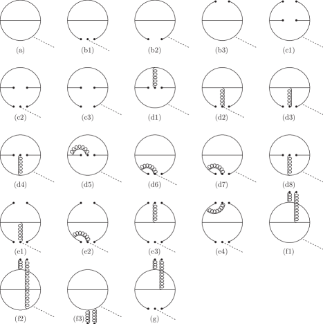
Figure 1: The diagrams that were used to calculate the Wilson coefficients of the correlation functions $\Pi_{\sigma}^{q}$ and $\Pi_{\sigma}^{1}$. The solid, wavy, and the dashed lines represent the quark, gluon, and the external scalar field, respectively.

Using the quark propagator in Eq. (12), one can compute the correlation function $\Pi^{\sigma}(q)$. The diagrams that we use to calculate the Wilson coefficients of $\Pi^{\sigma}(q)$ are shown in Fig. 1. Lorentz covariance and parity imply that $\Pi^{\sigma}(q)$ takes the form

$$\Pi^{\sigma}(q)=(\Pi_{\sigma}^{1}+\Pi_{\sigma}^{q}\hat{q})\sigma+(\Pi_{0}^{1}+\Pi_{0}^{q}\hat{q})\,,$$ (15)

where $\hat{q}=q^{\mu}\gamma_{\mu}$. Here $\Pi_{0}^{1}$ and $\Pi_{0}^{q}$ represent the invariant functions in the vicinity of the external field, which can be used to construct the mass sum rules for the nucleon, and $\Pi_{\sigma}^{1}$ and $\Pi_{\sigma}^{q}$ denote the invariant functions in the presence of the external field. Using these invariant functions, one can derive the sum rules at the structures $1$ and $\hat{q}$. $\Pi_{\sigma}^{q}$ and $\Pi_{\sigma}^{1}$ are evaluated as follows:

$$\Pi^{q}_{\sigma}(q)=g_{q}^{\sigma}\frac{1}{(2\pi)^{4}}\Big{[}a_{q}\,\ln(-q^{2})-\chi\,\frac{4}{3q^{2}}\,a_{q}^{2}+\frac{m_{0}^{2}}{2q^{2}}a_{q}-(\chi+\chi_{G})\,\frac{m_{0}^{2}}{6q^{4}}\,a_{q}^{2}\Big{]}\,,$$ (16)

and

$$\Pi^{1}_{\sigma}(q)=g_{q}^{\sigma}\frac{1}{(2\pi)^{4}} \Big{[}-\frac{q^{4}}{2}\ln(-q^{2})-\frac{10}{3q^{2}}a_{q}^{2}-\chi\,a_{q}\,q^{2}\ln(-q^{2})+\chi_{G}\frac{m_{0}^{2}}{2}a_{q}\,\ln(-q^{2})$$ (17)

$$~{}~{}+\frac{b}{8}\ln(-q^{2})-\chi\frac{b}{24q^{2}}a_{q}\Big{]}\,,$$

where we have defined $a_{q}\equiv-(2\pi)^{2}\langle\bar{q}q\rangle$, $b\equiv\langle g_{c}^{2}G^{2}\rangle$, and $m_{0}^{2}\equiv\langle g_{c}\bar{q}{\bm{\sigma}}\cdot{\bm{G}}q\rangle/\langle\bar{q}q\rangle$.

We now turn to the calculation of the hadronic side. We saturate the correlator in Eq. (7) with nucleon states and write

$$\Pi^{\sigma}(q)=\frac{\langle 0|\eta_{N}|N\rangle}{q^{2}-M_{N}^{2}}\,\,\langle N|\sigma N\rangle\,\,\frac{\langle N|\bar{\eta}_{N}|0\rangle}{q^{2}-M_{N}^{2}}\,\,,$$ (18)

where $M_{N}$ is the mass of the nucleon. The matrix element of the current $\eta_{N}$ between the vacuum and the nucleon state is defined as

$$\langle 0|\eta_{N}|N\rangle=\lambda_{N}\upsilon\,\,,$$ (19)

where $\lambda_{N}$ is the overlap amplitude and $\upsilon$ is the Dirac spinor for the nucleon, normalized as $\bar{\upsilon}\upsilon=2M_{N}$. Inserting Eq. (19) into Eq. (18) and defining $g_{N\!N\sigma}$  via the interaction Lagrangian density

$${\cal L}=-g_{N\!N\sigma}\,\bar{\upsilon}\upsilon\sigma\,\,,$$ (20)

we obtain for the hadronic part

$$-|\lambda_{N}|^{2}\frac{\hat{q}+M_{N}}{q^{2}-M_{N}^{2}}g_{N\!N\sigma}\frac{\hat{q}+M_{N}}{q^{2}-M_{N}^{2}}\,\,.$$ (21)

In addition, there are contributions coming from the excitations to higher nucleon states which are written as

$$-\lambda_{N}\lambda_{N^{\ast}}\,\frac{\hat{q}+M_{N}}{q^{2}-M_{N}^{2}}\,g_{N\!N^{\ast}\sigma}\,\frac{\hat{q}+M_{N^{\ast}}}{q^{2}-M_{N^{\ast}}^{2}}\,\,,$$ (22)

as well as contributions coming from the intermediate states due to $\sigma$-$N$ scattering, i.e. the continuum contributions. The term that corresponds to the excitations to higher nucleon states also has a pole at the nucleon mass, but a single pole instead of a double one like in Eq. (21). This single-pole term is not “damped” after the Borel transformation and should be included in the calculations.

Finally, there is another contribution that comes from the response of the continuum to the external field, given by

$$\int^{\infty}_{0}\frac{-\Delta s_{0}~{}b(s)}{s-q^{2}}\delta(s-s_{0})ds\,,$$ (23)

where $s_{0}$ is the continuum threshold, $\Delta s_{0}$ is the response of the continuum threshold to the external field, and $b(s)$ is a function that is calculated from the OPE. When $\Delta s_{0}$ is large, this term should also be included in the hadronic part Iof95 .

The QCD sum rules are obtained by matching the OPE side with the hadronic side and applying the Borel transformation. The resulting sum rules are:

$$\Big{[} -M^{4}\,a_{q}\,E_{0}+\frac{4}{3}\,\chi\,M^{2}\,a_{q}^{2}\,L^{4/9}-\frac{m_{0}^{2}}{2}\,M^{2}\,a_{q}\,L^{-14/27}-(\chi+\chi_{G})\,\frac{m_{0}^{2}}{6}\,a_{q}^{2}\,L^{-2/27}\Big{]}~{}e^{M_{N}^{2}/M^{2}}$$ (24)

$$~{}~{}~{}~{}~{}~{}=-\tilde{\lambda}_{N}^{2}\,\frac{M_{N}}{g_{q}^{\sigma}}\,g_{N\!N\sigma}+\tilde{B}_{q}\,\frac{M^{2}}{g_{q}^{\sigma}}+\frac{(s^{q}_{0})^{2}}{2g_{q}^{\sigma}}\,\Delta s^{q}_{0}\,M^{2}\,L^{-4/9}e^{(M_{N}^{2}-s_{0}^{q})/M^{2}}\,,$$

and

$$\Big{[} 2\,M^{8}\,E_{2}\,L^{-4/9}+\frac{20}{3}\,M^{2}\,a_{q}^{2}\,L^{4/9}+2\,\chi\,a_{q}\,M^{6}\,E_{1}-\chi_{G}\,m_{0}^{2}\,a_{q}\,M^{4}\,E_{0}\,L^{-14/27}$$ (25)

$$-\frac{b}{4}\,M^{4}\,E_{0}\,L^{-4/9}+\chi\,\frac{b}{12}\,M^{2}\,a_{q}\Big{]}~{}e^{M_{N}^{2}/M^{2}}$$

$$~{}~{}~{}~{}~{}~{}=-(2M_{N}^{2}-M^{2})\,\frac{\tilde{\lambda}_{N}^{2}}{g_{q}^{\sigma}}\,g_{N\!N\sigma}+\tilde{B}_{1}\,\frac{M^{2}}{g_{q}^{\sigma}}+\frac{4}{g_{q}^{\sigma}}\,a_{q}\,s^{1}_{0}\,\Delta s^{1}_{0}\,M^{2}\,e^{(M_{N}^{2}-s_{0}^{1})/M^{2}}\,,$$

where $M$ is the Borel mass and we have defined $\tilde{\lambda}_{N}^{2}=32\pi^{4}\lambda_{N}^{2}$. The continuum contributions are included by the factors

$$E_{0} \equiv 1-e^{-s_{0}^{i}/M^{2}}\,,$$

$$E_{1} \equiv 1-e^{-s_{0}^{i}/M^{2}}\Big{(}1+\frac{s_{0}^{i}}{M^{2}}\Big{)}\,,$$

$$E_{2} \equiv 1-e^{-s_{0}^{i}/M^{2}}\Big{(}1+\frac{s_{0}^{i}}{M^{2}}+\frac{(s_{0}^{i})^{2}}{2M^{4}}\Big{)}\,,$$ (26)

where $s_{0}^{i}$ are the continuum thresholds with $i=1,q$. In the sum rules above, we have included the single-pole contributions with the factors $\tilde{B}_{i}$. The third terms on the right-hand side (RHS) of Eqs. (24) and (25) denote the contributions that are explained in Eq. (23). These terms are suppressed by the factor $e^{-(s_{0}^{i}-M_{N}^{2})/M^{2}}$ as compared to the single-pole terms. We have incorporated the effects of the anomalous dimensions of the various operators through the factor $L=\ln(M^{2}/\Lambda_{QCD}^{2})/\ln(\mu^{2}/\Lambda_{QCD}^{2})$.

III Analysis of the sum rules and discussion

In this Section we analyze the sum rules derived in the previous Section in order to determine the value of $g_{N\!N\sigma}$ . We observe that the sum rule in Eq. (24) is more stable than the other sum rule in Eq. (25), so we use only this sum rule for the numerical analysis. Such a comparison and conclusion have been made about these sum rules also in some earlier works Jin93 ; Jin95 .

In order to calculate $g_{N\!N\sigma}$ , we need to know the values of the scalar susceptibilities $\chi$ and $\chi_{G}$. The value of the susceptibility $\chi$ can be calculated by using the two-point function Jin93

$$T(p^{2})=i\int d^{4}xe^{ip\cdot x}\Big{\langle}0\Big{|}{\cal T}[\bar{u}(x)u(x)+\bar{d}(x)d(x),\bar{u}(0)u(0)+\bar{d}(0)d(0)]\Big{|}0\Big{\rangle}\,,$$ (27)

via the relation

$$\chi\langle\bar{q}q\rangle=\frac{1}{2}T(0).$$ (28)

The two-point function in Eq. (27) at $p^{2}=0$ has been calculated in chiral perturbation theory Gas83 with the result

$$\chi=\frac{\langle\bar{q}q\rangle}{16\pi^{2}f_{\pi}^{4}}\Big{(}\frac{2}{3}\bar{\ell}_{1}+\frac{7}{3}\bar{\ell}_{2}-\frac{11}{6}\Big{)}\,,$$ (29)

where $f_{\pi}=93$ MeV is the pion decay constant and $\bar{\ell}_{1}$ and $\bar{\ell}_{2}$ are low-energy constants appearing in the effective chiral Lagrangian. The values of these low-energy constants have been estimated previously in various works (see e.g. Ref. Col01 for a review). A recent analysis of $\pi$-$\pi$ scattering gives $\bar{\ell}_{1}=-1.9\pm 0.2$ and $\bar{\ell}_{2}=5.25\pm 0.04$ Col01 , which is consistent with earlier determinations, but with smaller uncertainties. Using these values of $\bar{\ell}_{1}$ and $\bar{\ell}_{2}$ and taking the quark condensate $a_{q}=0.51\pm 0.03$ GeV³, we find $\chi=-10\pm 1$ GeV^-1. The value of the susceptibility $\chi_{G}$ is less certain. Therefore, we allow $\chi_{G}$ to vary in a wider range. We also adopt $b=4.7\times 10^{-1}$ GeV⁴, $\tilde{\lambda}_{N}^{2}=2.1$ GeV⁶, and $m_{0}^{2}=0.8$ GeV² Iof84 ; Ovc88 . We take $M_{N}=0.94$ GeV, the renormalization scale $\mu=0.5$ GeV, and the QCD scale parameter $\Lambda_{QCD}=0.1$ GeV. It is relevant to point out that the choice of the two-point function in Eq. (27) does not imply a theoretical prejudice about the structure of the scalar mesons. What is calculated is just the susceptibility pertaining to the response of the quark condensates $\langle\bar{q}q\rangle$ to the scalar $q\bar{q}$ field, as shown in Eq. (II).

To proceed to the numerical analysis, we arrange the RHS of Eq. (24) in the form

$$f(M^{2})=A_{q}+B_{q}M^{2}+C_{q}M^{2}L^{-4/9}e^{(M_{N}^{2}-s_{0}^{q})/M^{2}}\ ,$$ (30)

and fit the left-hand side (LHS) to $f(M^{2})$. Here we have defined

$$A_{q} \equiv -\tilde{\lambda}_{N}^{2}\frac{M_{N}}{g_{q}^{\sigma}}g_{N\!N\sigma}\,,$$

$$B_{q} \equiv \frac{\tilde{B}_{q}}{g_{q}^{\sigma}}\,,$$

$$C_{q} \equiv \frac{(s^{q}_{0})^{2}}{2g_{q}^{\sigma}}\Delta s^{q}_{0}\,.$$ (31)

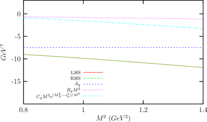
Figure 2: (Color online) The Borel mass dependence of LHS and the fitted RHS of Eq. (24) for $s^{q}_{0}=2.3$ GeV² and $\chi_{G}\equiv\chi=-10$ GeV^-1. We also present the terms on the RHS individually. Note that the LHS curve (solid) overlies the RHS curve (dashed).

In Fig. 2, we present the Borel mass dependence of the LHS and the RHS of Eq. (24) for $s^{q}_{0}=2.3$ and $\chi_{G}\equiv\chi=-10$ GeV^-1. We choose the Borel window 0.8 GeV² $\leq M^{2}\leq 1.4$ GeV² which is commonly identified as the fiducial region for the nucleon mass sum rules Iof84 . It is seen that the LHS curve (solid) overlies the RHS curve (dashed). In order to estimate the contributions that come from the excited nucleon states and the response of the continuum threshold, we plot each term on the RHS individually. We observe that the single-pole terms (dotted) give very small contribution, but the response of the continuum threshold (dot-dashed) is quite sizable. Nevertheless, the summation of these curves with the line of the double-pole term (small-dashed) gives a stable sum rule.

In Fig. 3, we plot the Borel mass dependence of the four terms on the LHS of Eq. (24) separately, together with their summation for $s^{q}_{0}=2.3$ GeV² and $\chi_{G}\equiv\chi=-10$ GeV^-1. This helps us to compare the contributions of different operators on the OPE side. Here ${\cal O}_{1}$ denotes the first term, ${\cal O}_{2}$ denotes the second term, and so on. We observe that ${\cal O}_{1}$ and ${\cal O}_{3}$ are small, ${\cal O}_{4}$ is sizable, and ${\cal O}_{2}$ is large. The term ${\cal O}_{4}$ contributes with different sign with respect to ${\cal O}_{1}$ and ${\cal O}_{3}$, and so tends to cancel the latter. Therefore $g_{N\!N\sigma}$  is mainly determined by ${\cal O}_{2}$ on the LHS.

In order to see the sensitivity of the coupling constant on the continuum threshold and the susceptibility $\chi$, we plot in Fig. 4 the dependence of $g_{N\!N\sigma}/g_{q}^{\sigma}$ on $\chi$ for three different values $s_{0}^{q}=2.0$, 2.3, and 2.5 GeV², and taking $\chi\equiv\chi_{G}$. One sees that $g_{N\!N\sigma}$  changes by approximately $8\%$ in the considered region of the susceptibility $\chi$. The value of $g_{N\!N\sigma}$  is not very sensitive to a change in $s_{0}^{q}$, which gives an uncertainty of approximately $6\%$ to the final value. Taking into account the uncertainty in $\chi$, $s_{0}^{q}$, and $a_{q}$, the predicted value for $g_{N\!N\sigma}/g_{q}^{\sigma}$ of the sum rule in Eq. (24) reads

$$g_{N\!N\sigma}/g_{q}^{\sigma}=3.9\pm 1.0\,.$$ (32)

In a similar way, one can calculate the other two terms on the RHS of Eq. (24) as:

$$B_{q} = -0.2\pm 1.2~{}\text{GeV}^{5}\,,$$

$$C_{q} = -7.9\pm 2.9~{}\text{GeV}^{5}\,.$$ (33)

As noted above, the value of the susceptibility $\chi_{G}$ is less certain than the value of $\chi$. If we let $\chi_{G}$ change in a wider range, say $6~{}\text{GeV}^{-1}\leq-\chi_{G}\leq 14~{}\text{GeV}^{-1}$, this brings an additional $15\%$ uncertainty to the value quoted in Eq. (32).

The ratio in Eq. (32) is in agreement with the naive quark model, which gives $g_{N\!N\sigma}/g_{q}^{\sigma}=3$ based on counting the $u$- and the $d$-quarks in the nucleon. (Ideal mixing in the scalar sector is assumed above, that is, the sigma meson is taken without a strange-quark content.) Another estimate can be made from the ratio of pion-nucleon to pion-quark coupling constant, $g_{N\!N\pi}/g_{q}^{\pi}$. Since the $\sigma$ meson is the chiral partner of the pion Wei90 , one expects

$$g_{N\!N\sigma}/g_{q}^{\sigma}=g_{N\!N\pi}/g_{q}^{\pi}\,.$$ (34)

Using the Goldberger-Treiman relation for both the pion-nucleon and the pion-constituent quark couplings,

$$g_{N\!N\pi} = g^{A}_{N}\frac{M_{N}}{f_{\pi}}\,,$$

$$g_{q}^{\pi} = g^{A}_{q}\frac{m_{q}}{f_{\pi}}\,,$$ (35)

where $m_{q}$ is the mass of the constituent quark, $g^{A}_{N}$ and $g^{A}_{q}$ are the nucleon and the quark axial couplings, respectively, one obtains Glo95

$$\frac{g_{N\!N\pi}}{g_{q}^{\pi}}=\frac{5}{3}\frac{M_{N}}{m_{q}}\,.$$ (36)

With a constituent-quark mass of 340 MeV Glo95 , Eq. (36) yields $g_{N\!N\pi}/g_{q}^{\pi}=4.6$. Using Eq. (34) we find that this agrees nicely with the QCDSR result in Eq. (32).

To determine $g_{N\!N\sigma}$ , one next has to assume some value for the quark-$\sigma$ coupling constant $g_{q}^{\sigma}$. Adopting the value $g_{q}^{\sigma}=3.7$ as estimated from the sigma model Ris99 , we obtain

$$g_{N\!N\sigma}=14.4\pm 3.7\,.$$ (37)

The coupling constant in Eq. (37) is defined at $t=0$, i.e. $g_{N\!N\sigma}\equiv g_{N\!N\sigma}(t=0)$. As stressed above, also in NN potential models the heavy-meson coupling constants are determined at $t=0$. The (large) value of $g_{N\!N\sigma}$  obtained in Eq. (37) is in agreement with the value $g_{N\!N\sigma}=16.9$ from the Nijmegen soft-core NN potential model Nag78 , obtained from a fit to the NN scattering data.

IV Conclusion

We have calculated the coupling constant $g_{N\!N\sigma}$  of the isoscalar-scalar meson, which plays a significant role in OBE models of the NN and YN interactions, to the nucleon, using the external-field QCDSR method. Our main result is the ratio $g_{N\!N\sigma}/g_{q}^{\sigma}$ in Eq. (32) which is determined purely from QCDSR. The value of $g_{N\!N\sigma}$  is dependent on $g_{q}^{\sigma}$, the value of which we use as estimated in the sigma model. The obtained value of $g_{N\!N\sigma}$  is in agreement with the large value found in OBE models. We have also computed the contributions that come from the excited nucleon states and the response of the continuum threshold to the external field. We observe that while the single-pole contributions are small, the response of the continuum threshold is sizable. We plan to extend the external-field QCDSR method to the hyperons and the complete scalar-meson nonet, in order to address the $SU(3)$-flavor structure of the scalar-meson coupling constants to the baryon octet Erkol .

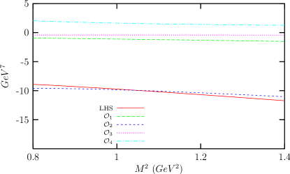
Figure 3: (Color online) The four terms on the LHS of Eq. (24) individually, together with the summation of them for $s^{q}_{0}=2.3$ GeV² and $\chi_{G}\equiv\chi=-10$ GeV^-1. Here ${\cal O}_{1}$ denotes the first term, ${\cal O}_{2}$ denotes the second term, and so on.

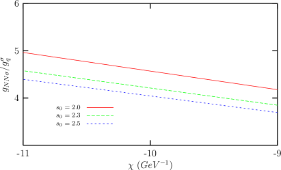
Figure 4: (Color online) The dependence of $g_{N\!N\sigma}/g_{q}^{\sigma}$ on the susceptibility $\chi$ for three different values of $s_{0}^{q}=2.0$, 2.3, and 2.5 GeV²; here we take $\chi\equiv\chi_{G}$.

- (1) M. M. Nagels, T. A. Rijken, and J. J. de Swart, Phys. Rev. D 17, 768 (1978).
- (2) V. G. J. Stoks, R. A. M. Klomp, C. P. F. Terheggen, and J. J. de Swart, Phys. Rev. C 49, 2950 (1994).
- (3) P. M. M. Maessen, Th. A. Rijken, and J. J. de Swart, Phys. Rev. C 40, 2226 (1989).
- (4) Th. A. Rijken, V. G. J. Stoks, and Y. Yamamoto, Phys. Rev. C 59, 21 (1999) [arXiv:nucl-th/9807082].
- (5) R. G. E. Timmermans, Th. A. Rijken, and J. J. de Swart, Phys. Rev. C 50, 48 (1994) [arXiv:nucl-th/9403011].
- (6) J. J. de Swart, P. M. M. Maessen, and T. A. Rijken, in: Properties and Interactions of Hyperons, edited by B. F. Gibson, P. D. Barnes, and K. Nakai (World Scientific, Singapore, 1994), pp. 37-54 [arXiv:nucl-th/9405008].
- (7) J. Binstock and R. Bryan, Phys. Rev. D 4, 1341 (1971); R. A. Bryan and A. Gersten, Phys. Rev. D 6, 341 (1972).
- (8) S. Weinberg, Phys. Rev. Lett. 65, 1177 (1990).
- (9) E. van Beveren, T. A. Rijken, K. Metzger, C. Dullemond, G. Rupp, and J. E. Ribeiro, Z. Phys. C 30, 615 (1986); E. van Beveren, G. Rupp, T. A. Rijken, and C. Dullemond, Phys. Rev. D 27, 1527 (1983).
- (10) R. L. Jaffe, Phys. Rev. D 15, 281 (1977); Phys. Rev. D 17, 1444 (1978).
- (11) A. T. M. Aerts, P. J. Mulders, and J. J. de Swart, Phys. Rev. D 21, 1370 (1980).
- (12) D. Black, A. H. Faziborz, F. Sannino, and J. Schechter, Phys. Rev. D 59, 074026 (1999) [arXiv:hep-ph/9808415].
- (13) L. Maiani, F. Piccinini, A. D. Polosa, and V. Riquer, Phys. Rev. Lett. 93, 212002 (2004) [arXiv:hep-ph/0407017].
- (14) T. V. Brito, F. S. Navarra, M. Nielsen and M. E. Bracco, Phys. Lett. B 608, 69 (2005) [arXiv:hep-ph/0411233].
- (15) M. A. Shifman, A. I. Vainshtein, and V. I. Zakharov, Nucl. Phys. B147, 385 (1979); Nucl. Phys. B147, 448 (1979).
- (16) L. J. Reinders, H. Rubinstein, and S. Yazaki, Phys. Rept. 127, 1 (1985).
- (17) P. Colangelo and A. Khodjamirian, in: Boris Ioffe Festschrift ’At the Frontier of Particle Physics / Handbook of QCD’ vol.3, edited by M. Shifman (World Scientific, Singapore, 2001).
- (18) K. Maltman, Phys. Rev. C 57, 69 (1998) [arXiv:hep-ph/9707231].
- (19) B. L. Ioffe and A. V. Smilga, Nucl. Phys. B232, 109 (1984).
- (20) I. I. Balitsky and A. V. Yung, Phys. Lett. B 129, 328 (1983).
- (21) C. B. Chiu, J. Pasupathy, and S. L. Wilson, Phys. Rev. D 33, 1961 (1986).
- (22) C. B. Chiu, J. Pasupathy, and S. L. Wilson, Phys. Rev. D 32, 1786 (1985).
- (23) V. M. Belyaev and Y. I. Kogan, Phys. Lett. B 136, 273 (1984).
- (24) X. M. Jin, M. Nielsen, and J. Pasupathy, Phys. Lett. B 314, 163 (1993).
- (25) X. M. Jin, Phys. Rev. D 52, 2964 (1995) [arXiv:hep-ph/9506299]; X. M. Jin, M. Nielsen, and J. Pasupathy, Phys. Rev. D 51, 3688 (1995) [arXiv:hep-ph/9405202].
- (26) H. Shiomi and T. Hatsuda, Nucl. Phys. A594, 294 (1995) [arXiv:hep-ph/9504354].
- (27) M. C. Birse and B. Krippa, Phys. Rev. C 54, 3240 (1996) [arXiv:hep-ph/9606471].
- (28) H. C. Kim, S. H. Lee and M. Oka, Phys. Lett. B 453 (1999) 199 [arXiv:nucl-th/9809004].
- (29) H. C. Kim, S. H. Lee and M. Oka, Phys. Rev. D 60 034007 (1999) [arXiv:nucl-th/9811096].
- (30) H. C. Kim, T. Doi, M. Oka, and S. H. Lee, Nucl. Phys. A662, 371 (2000) [arXiv:nucl-th/9909007]; Nucl. Phys. A678, 295 (2000) [arXiv:nucl-th/0002011].
- (31) W. Y. Hwang, Z. Phys. C 75, 701 (1997) [arXiv:hep-ph/9601219].
- (32) W. Y. Hwang, Z. s. Yang, Y. S. Zhong, Z. N. Zhou and S. L. Zhu, Phys. Rev. C 57, 61 (1998) [arXiv:nucl-th/9610025].
- (33) E. M. Henley, W. Y. P. Hwang, and L. S. Kisslinger, Phys. Lett. B 367, 21 (1996); ibid. B 440, 449(E) (1998) [arXiv:nucl-th/9511002].
- (34) Y. Wen and W. Y. P. Hwang, Phys. Rev. C 56, 3346 (1997).
- (35) D. B. Kaplan and A. V. Manohar, Phys. Rev. C 56, 76 (1997) [arXiv:nucl-th/9612021].
- (36) J. J. de Swart and M. M. Nagels, Fortsch. Phys. 26, 215 (1978).
- (37) B. L. Ioffe, Nucl. Phys. B188, 317 (1981); ibid. B191, 591(E) (1981).
- (38) B. L. Ioffe, Phys. Atom. Nucl. 58, 1408 (1995) [Yad. Fiz. 58N8, 1492 (1995)] [arXiv:hep-ph/ 9501319].
- (39) J. Gasser and H. Leutwyler, Ann. Phys. 158, 142 (1984).
- (40) G. Colangelo, J. Gasser, and H. Leutwyler, Nucl. Phys. B603, 125 (2001) [arXiv:hep-ph/0103088].
- (41) A. A. Ovchinnikov and A. A. Pivovarov, Sov. J. Nucl. Phys. 48, 721 (1988).
- (42) L. Y. Glozman and D. O. Riska, Phys. Rep. 268, 263 (1996) [arXiv:hep-ph/9505422].
- (43) D. O. Riska and G. E. Brown, Nucl. Phys. A653, 251 (1999) [arXiv:hep-ph/9902319].
- (44) G. Erkol, Th. A. Rijken, and R. G. E. Timmermans, in preparation.