Extended-soft-core Baryon-Baryon Model
II. Hyperon-Nucleon Interaction

Abstract

The YN results are presented from the Extended-soft-core (ESC) interactions. They consist of local- and non-local-potentials due to (i) One-boson-exchanges (OBE), which are the members of nonets of pseudoscalar-, vector-, scalar-, and axial-mesons, (ii) Diffractive exchanges, (iii) Two pseudoscalar exchange (PS-PS), and (iv) Meson-Pair-exchange (MPE). Both the OBE- and Pair-vertices are regulated by gaussian form factors producing potentials with a soft behavior near the origin. The assignment of the cut-off masses for the BBM-vertices is dependent on the SU(3)-classification of the exchanged mesons for OBE, and a similar scheme for MPE.

The particular version of the ESC-model, called ESC04 Rij04a , describes nucleon-nucleon (NN) and hyperon-nucleon (YN) in a unified way using broken SU(3)-symmetry. Novel ingredients are the inclusion of (i) the axial-vector meson potentials, (ii) a zero in the scalar- and axial-vector meson form factors. These innovations made it possible for the first time to keep the parameters of the model closely to the predictions of the ${}^{3}P_{0}$ quark-antiquark creation (QPC) model. This is also the case for the $F/(F+D)$-ratio’s. Furthermore, the introduction of the zero helped to avoid the occurrence of unwanted bound states.

Broken SU(3)-symmetry serves to connect the NN and the YN channels, which leaves after fitting NN only a few free parameters for the determination of the YN-interactions. In particular, the meson-baryon coupling constants are calculated via SU(3) using the coupling constants of the NN-analysis as input. Here, as a novel feature, we allow for medium strong flavor-symmetry-breaking (FSB) of the coupling constants, using the ${}^{3}P_{0}$-model with a Gell-Mann-Okubo hypercharge breaking for the BBM-coupling. We obtained very good fits for ESC-model with and without FSB. The charge-symmetry-breaking (CSB) in the $\Lambda p$ and $\Lambda n$ channels, which is an SU(2) isospin breaking, is included in the OBE-, TME-, and MPE-potentials.

We describe simultaneous fits to the NN- and the YN- scattering data, using different options for the ESC-model. For the selected 4233 NN-data with energies $0\leq T_{lab}\leq 350$ MeV, we typically reached a $\chi^{2}/N_{\rm data}=1.22$. For the usual set of 35 YN-data and 3 $\Sigma^{+}p$ cross-sections from a recent KEK-experiment E289 Kanda05 we obtained $\chi^{2}/{\it YN}_{\rm data}\approx 0.63$. In particular, we were able to fit the precise experimental datum $r_{R}=0.468\pm 0.010$ for the inelastic capture ratio at rest rather well.

The four versions (a,b,c,d) of ESC04 presented in this paper, give different results for hypernuclei. The reported G-matrix calculations are performed for YN ($\Lambda N$, $\Sigma N$, $\Xi N$) pairs in nuclear matter. The obtained well depths ($U_{\Lambda}$, $U_{\Sigma}$, $U_{\Xi}$) reveal distinct features of ESC04a-d. The $\Lambda\Lambda$-interactions are demonstrated to be consistent with the observed data of ${}^{\ 6}_{\Lambda\Lambda}$He. The possible three-body effects are investigated by considering phenomenologically the changes of the vector-meson masses.

I Introduction

This is the second in a series of papers where we present the recent results obtained with the Extended-Soft-Core model, henceforth referred to as ESC04, model for nucleon-nucleon (NN), hyperon-nucleon (YN), and hyperon-hyperon (YY). This paper treats the N​N- and Y​N(S=-1)-systems. In Rij04a , in the following referred to as I, many formal aspects have been described or discussed rather extensively. Therefore, in this paper we will concentrate on items that are in particularly important in YN, and that were not treated in Rij04a . In paper III Rij04c the $S=-2$ channels will be described.

In MRS89 and RSY99 it has been shown the a soft-core (SC) one-boson-exchange (OBE) model, based on regge-pole theory Rij85 , provides a satisfactory description of many aspects of the nucleon-nucleon (N​N) and hyperon-nucleon (Y​N) channels.

Since for N​N the ESC-model has given a big step forward in the detailed description, one may expect that a simultaneous and unified treatment of the N​N and Y​N channels, using broken SU(3), will give a very realistic model for the baryon-baryon interactions. (In this paper by SU(3) is meant always SU(3)-flavor.)

In all previous work of the Nijmegen group, the exploration of (broken) SU(3)-symmetry connects the N​N and the Y​N channels, leaving after fitting ${\it N\!N}$ only a few free parameters to be determined in the YN-interactions. The latter is important in view of the scarce experimental Y​N-data. In particular, the baryon-baryon-meson BBM coupling constants are calculated via SU(3) using the coupling constants of the N​N-analysis as input. The first versions of the ESC-model, referred to as ESC00 Rij00 ; Rij01 , worked along the same procedures. The aim of the ESC00 work was to demonstrate the ability of the ESC-model to realize a very good description of the N​N- and Y​N-data, i.e. a low $\chi^{2}$. Therefore, we left much freedom to the parameters. However, in the ESC04 version presented here, we focus on the improvement of the physics of the model by restricting the coupling constants in the BBM-vertices by the predictions of the quark-model (QM) in the form of the ${}^{3}P_{0}$ antiquark-quark pair creation model (QPC) Mic69 . Also, all $\alpha=F/(F+D)$-ratios are taken close to the QPC-model predictions for the BBM- and the B​B-Pair-vertices. An exception is made here for the pseudoscalar $\alpha_{PV}$ and the $\alpha_{V}^{m}$ ratios. The first because it is interesting to see how close or different it becomes as compared to the same ratio in weak interactions, where $\alpha_{PV}=0.355$. The second, because it proved to be an important regulator for the S-wave spin-dependence of the $\Lambda N$-interaction RSY99 .

In MRS89 the magnetic ratio $\alpha_{V}^{m}$ for the vector-mesons was fixed to its SU(6)-value, but the spin-spin interaction needed a correction. This because the S-wave spin-spin interaction in the $\Lambda N$-channels became later well known from hypernuclear systems Yam90 ; Mot95 ; Has95 . In RSY99 , to improve the spin-spin interaction, we left $\alpha_{V}^{m}$ free and made fits for different values of this parameter. It turned out that in this way we indeed can construct soft-core Y​N-models which encompass a range of scattering length’s in the ${}^{1}S_{0}$ and the ${}^{3}S_{1}$ $\Lambda N$ channels. From the NSC97a-f models the sensitivity with respect to $\alpha^{m}_{V}$ is evident.

SU(3)-symmetry and the QPC-model give strong constraints on the coupling parameters. In order to keep some more flexibility in distinguishing the N​N- and the Y​N(S=-1)-channels, similarly to the NSC97 models RSY99 , we allow for medium strong breaking of the coupling constants, employing again the ${}^{3}P_{0}$-model with a Gell-Mann-Okubo hypercharge breaking for the BBM-coupling. This leads to a universal scheme for SU(3)-breaking of the coupling constants for all meson nonets, in terms of a single extra parameter.

To summarize the different sources of SU(3)-breaking, we include (i) using the physical masses of the mesons and baryons in the potentials and Schrödinger equation, (ii) allowing for meson-mixing within a nonet $(\eta-\eta^{\prime},\ \omega-\phi,\ \varepsilon-f^{\prime}_{0}$, (iii) including Charge Symmetry Breaking (CSB) Dal64 due to $\Lambda\Sigma$-mixing, which for example introduces a one-pion-exchange (OPE) potential in the $\Lambda N$ channel, (iv) taking into account the Coulomb-interaction.

The electromagnetic SU(2)-breaking Dal64 , called Charge-Symmetry-Breaking (CSB), in the $\Lambda p$ and $\Lambda n$ channels is included, not only for the BBM- but also for the BB-Pair-couplings.

The BBM-vertices are described by coupling constants and form factors, which correspond to the regge residues at high energies Rij85 . The form factors are taken to be of the gaussian-type, like the residue functions in many regge-pole models for high energy scattering. Note that also in (nonrelativistic) quark models (QM’s) a gaussian behavior of the form factors is most natural. These form factors evidently guarantee a soft behavior of the potentials in configuration space at small distances.

In RSY99 the assignment of the cut-off parameters in the form factors was made for the individual baryon-baryon-meson (BBM) vertices, constrained by broken SU(3)-symmetry. This in distinction to the first attempt to construct soft-core interaction MRS89 , where cut-offs were assigned per baryon-baryon SU(3)-irrep. The latter scheme we consider now not natural and we use here the same scheme as in RSY99 . Moreover, this way we obtain immediately full predictive power for the $S=-2$ etc. baryon-baryon channels, e.g. $\Lambda\Lambda,\Xi N$-channels which involve the singlet $\{1\}$-irrep that does not occur in the N​N and Y​N channels.

The dynamics of the ESC04 model has been described and discussed in paper I Rij04a , and it is sufficient to refer to this here for all types of exchanges that are included. Nevertheless, some more remarks on the scalar mesons are appropriate. An extensive discussion of the situation with respect to the scalar mesons is given in RSY99 . The question whether the $J^{PC}=0^{++}$-mesons are of the Dalitz-type ($Q\bar{Q}$) or of the Jaffe-type ($Q^{2}\bar{Q}^{2}$) is not yet decided. In the coupling to the baryons, we assume here that the basic process is described by the QPC-model Mic69 . It has been shown in paper I that this seems rather successful, justifying this assumption.

With a combined treatment of the $N\!N$ and $Y\!N$ channels we aim at a high quality description of the baryon-baryon interactions. By high quality we understand here a ${\it YN}$-fit with low $\chi^{2}$ and such that, while keeping the constraints forced on the potentials by the ${\it NN}$-fit, the free parameters with a clear physical significance, like e.g. the $F/(F+D)$-ratio’s $\alpha_{PV}$ and $\alpha_{V}^{m}$, assume realistic values.

Such a combined study of all baryon-baryon interactions, and especially N​N and Y​N, is desirable if one wants:

• To study the assumption of broken SU(3)-symmetry. For example we want to investigate the properties of the scalar mesons ($\varepsilon(760)$, $f_{0}(975)$, $a_{0}(980)$, $\kappa(1000)$). We note that especially the status of the scalar nonet is at present not established yet.

• To determination of $F/(F+D)$-ratio’s.

• To extract, in spite of the scarce experimental ${\it YN}$-data, information about scattering lengths, effective ranges, the existence of resonances etc.

• To provide realistic baryon-baryon potentials, which can be applied in few-body computations, nuclear- and hyperonic matter studies.

• To extend the theoretical description to the $\Lambda\Lambda$ and $\Xi N$ channels, where experiments may be realized in the foreseeable future.

In the construction of the ESC-models there are two important options:

1. First, there is the choice of the pv- or the ps-coupling for the pseudoscalar mesons, or some mixture, regulated by the $a_{PV}$-parameter, of these. This choice affects some $1/M^{2}$-terms in the ps-ps-exchange potentials.

2. Second, yes or no medium strong symmetry-breaking of the couplings, regulated by a $\Delta_{FSB}$-parameter.

We have accordingly produced four different solutions, fitting simultaneously the ${\it NN}\oplus{\it YN}$-data, which are referred to as follows: ESC04a$(\Delta_{FSB}\neq 0,a_{PV}=0.5)$, ESC04b$(\Delta_{FSB}\neq 0,a_{PV}=1.0)$, ESC04c$(\Delta_{FSB}=0,a_{PV}=0.5)$, ESC04d$(\Delta_{FSB}=0,a_{PV}=1.0)$. Here, $a_{PV}=1.0$ and $a_{PV}=0.0$ means pure pseudo-vector respectively purely pseudoscalar coupling. It appears that there are notable differences between these models, in particularly their properties for matter, e.g. well-dephs $U_{\Lambda},U_{\Sigma}$, and $U_{\Xi}$, are rather distinct.
We will display and discuss in this paper only the results for the ESC04a-model in detail. With the exception of the G-matrix results, we will be very brief on ESC04b-d and will compare these models only very globally. So, in the following, by ESC04 is meant ESC04a, unless specified otherwise.

As in all Nijmegen models, the Coulomb interaction is included exactly, for which we solve the multichannel Schrödinger equation on the physical particle basis. The nuclear potentials are calculated on the isospin basis, in order to limit the number of different form factors. This means that we include only the so-called ’medium strong’ SU(3)-breaking in the potentials.

The contents of this paper are as follows. In section II we describe the $S=-1$ $Y\!N$-channels on the isospin and particle basis, and the use of the multi-channel Schrödinger equation is mentioned. The potentials in momentum and configuration space are defined by referring to the description given in paper I. The BBM-couplings are discussed both in the $3\times 3$-matrix and the cartesian-octet representation. The SU(3)-couplings of the OBE- and TME-graphs are given in a form suitable for a digital evaluation.
In section III the meson-pair interaction Hamiltonians are given in the context of SU(3). Expressions for the meson-pair-exchange (MPE) graphs are given, again in an immediately programmable form. In section IV the medium-strong breaking of SU(3)-symmetry of the coupling constants is described. The QPC-model is employed for the development of a universal scheme for this breaking. Here also the detailed prescription for the handling of the cut-off parameters is given, in particularly for the cases of meson-mixing.
In section V the simultaneous ${\it NN}\oplus{\it YN}$ fitting procedure is reviewed. In section VI the results for the coupling constants and $F/(F+D)$-ratios for OBE and MPE are given. They are discussed and compared with the predictions of the QPC-model. Here, also the values of the $BBM$-couplings are displayed for pseudoscalar, vector, scalar, and axial-vector mesons.
In section VII the NN-results from the combined ${\it NN}\oplus{\it YN}$-fit, model ESC04a, henceforth called ESC04, are discussed and compared with the results of paper I, referred to ESC04(NN). In section VIII we discuss the fit to the Y​N scattering data from the combined ${\it NN}\oplus{\it YN}$-fit. In section IX we compare very briefly the models ESC04a-d.
In section X, the hypernuclear properties of ESC04a-d are studied through the G-matrix calculations for YN ($\Lambda N$, $\Sigma N$, $\Xi N$) and their partial-wave contributions. Here, the implications of possible three-body effects for the nuclear saturation and baryon well-dephs are discussed. Also, the $\Lambda\Lambda$ interactions in ESC04a-d are demonstrated to be consistent with the observed data of ${}^{\ 6}_{\Lambda\Lambda}$He. In section XI we finish by a final discussion and draw some conclusions.

II Channels, Potentials, and SU(3)-symmetry

II.1 Channels and Potentials

In this paper we consider the hyperon-nucleon reactions with $S=-1$

$$Y(p_{a},s_{a})+N(p_{b},s_{b})\rightarrow Y(p^{\prime}_{a},s^{\prime}_{a})+N(p^{\prime}_{b},s^{\prime}_{b})$$ (1)

Like in Ref.’s MRS89 ; RSY99 we will also refer to $Y$ and $Y^{\prime}$ as particles 1 and 3, and to $N$ and $N^{\prime}$ as particles 2 and 4. For the kinematics and the definition of the amplitudes, we refer to paper I Rij04a of this series. Similar material can be found in MRS89 . Also, in paper I the derivation of the Lippmann-Schwinger equation in the context of the relativistic two-body equation is described.

On the physical particle basis, there are four charge channels:

$$q=+2:\ \ \Sigma^{+}p\rightarrow\Sigma^{+}p,$$

$$q=+1:\ \ (\Lambda p,\Sigma^{+}n,\Sigma^{0}p)\rightarrow(\Lambda p,\Sigma^{+}n,\Sigma^{0}p),$$

$$q=\ \ 0:\ \ (\Lambda n,\Sigma^{0}n,\Sigma^{-}p)\rightarrow(\Lambda n,\Sigma^{0}n,\Sigma^{-}p),$$

$$q=-1:\ \ \Sigma^{-}n\rightarrow\Sigma^{-}n.$$ (2)

Like in MRS89 ; RSY99 , the potentials are calculated on the isospin basis. For $S=-1$ hyperon-nucleon systems there are only two isospin channels: (i) $I={\textstyle\frac{1}{2}}:\ \ (\Lambda N,\Sigma N\rightarrow\Lambda N,\Sigma N)$, and (ii) $I={\textstyle\frac{3}{2}}:\ \ \Sigma N\rightarrow\Sigma N$.

Obviously, the potential on the particle basis for the $q=2$ and $q=-1$ channels are given by the $I={\textstyle\frac{3}{2}}$ $\Sigma N$ potential on the isospin basis. For $q=1$ and $q=0$, the potentials are related to the potentials on the isospin basis by an isospin rotation. Using a notation where we only list the hyperons [$V_{\Lambda\Sigma^{+}}=(\Lambda p|V|\Sigma^{+}n)$, etc.], we find for $q=1$

$$\left(\begin{array}[]{ccc}V_{\Lambda\Lambda}&V_{\Lambda\Sigma^{+}}&V_{\Lambda\Sigma^{0}}\\[5.69054pt] V_{\Sigma^{+}\Lambda}&V_{\Sigma^{+}\Sigma^{+}}&V_{\Sigma^{+}\Sigma^{0}}\\[5.69054pt] V_{\Sigma^{0}\Lambda}&V_{\Sigma^{0}\Sigma^{+}}&V_{\Sigma^{0}\Sigma^{0}}\end{array}\right)=\left(\begin{array}[]{ccc}V_{\Lambda\Lambda}&\sqrt{\textstyle\frac{2}{3}}V_{\Lambda\Sigma}&-\sqrt{\textstyle\frac{1}{3}}V_{\Lambda\Sigma}\\[5.69054pt] \sqrt{\textstyle\frac{2}{3}}V_{\Sigma\Lambda}&{\textstyle\frac{2}{3}}V_{\Sigma\Sigma}({\textstyle\frac{1}{2}})+{\textstyle\frac{1}{3}}V_{\Sigma\Sigma}({\textstyle\frac{3}{2}})&{\textstyle\frac{1}{3}}\sqrt{2}\left[V_{\Sigma\Sigma}({\textstyle\frac{3}{2}})-V_{\Sigma\Sigma}({\textstyle\frac{1}{2}})\right]\\[5.69054pt] -\sqrt{\textstyle\frac{1}{3}}V_{\Sigma\Lambda}&{\textstyle\frac{1}{3}}\sqrt{2}\left[V_{\Sigma\Sigma}({\textstyle\frac{3}{2}})-V_{\Sigma\Sigma}({\textstyle\frac{1}{2}})\right]&{\textstyle\frac{1}{3}}V_{\Sigma\Sigma}({\textstyle\frac{1}{2}})+{\textstyle\frac{2}{3}}V_{\Sigma\Sigma}({\textstyle\frac{3}{2}})\end{array}\right)\ ,$$ (3)

while for $q=0$ we find

$$\left(\begin{array}[]{ccc}V_{\Lambda\Lambda}&V_{\Lambda\Sigma^{0}}&V_{\Lambda\Sigma^{-}}\\[5.69054pt] V_{\Sigma^{0}\Lambda}&V_{\Sigma^{0}\Sigma^{0}}&V_{\Sigma^{0}\Sigma^{-}}\\[5.69054pt] V_{\Sigma^{-}\Lambda}&V_{\Sigma^{-}\Sigma^{0}}&V_{\Sigma^{-}\Sigma^{-}}\end{array}\right)=\left(\begin{array}[]{ccc}V_{\Lambda\Lambda}&\sqrt{\textstyle\frac{1}{3}}V_{\Lambda\Sigma}&-\sqrt{\textstyle\frac{2}{3}}V_{\Lambda\Sigma}\\[5.69054pt] \sqrt{\textstyle\frac{1}{3}}V_{\Sigma\Lambda}&{\textstyle\frac{1}{3}}V_{\Sigma\Sigma}({\textstyle\frac{1}{2}})+{\textstyle\frac{2}{3}}V_{\Sigma\Sigma}({\textstyle\frac{3}{2}})&{\textstyle\frac{1}{3}}\sqrt{2}\left[V_{\Sigma\Sigma}({\textstyle\frac{3}{2}})-V_{\Sigma\Sigma}({\textstyle\frac{1}{2}})\right]\\[5.69054pt] -\sqrt{\textstyle\frac{2}{3}}V_{\Sigma\Lambda}&{\textstyle\frac{1}{3}}\sqrt{2}\left[V_{\Sigma\Sigma}({\textstyle\frac{3}{2}})-V_{\Sigma\Sigma}({\textstyle\frac{1}{2}})\right]&{\textstyle\frac{2}{3}}V_{\Sigma\Sigma}({\textstyle\frac{1}{2}})+{\textstyle\frac{1}{3}}V_{\Sigma\Sigma}({\textstyle\frac{3}{2}})\end{array}\right)\ .$$ (4)

For the kinematics of the reactions and the various thresholds, see RSY99 . In this work we do not solve the Lippmann-Schwinger equation, but the multi-channel Schrödinger equation in configuration space, completely analogous to MRS89 . The multichannel Schrödinger equation for the configuration-space potential is derived from the Lippmann-Schwinger equation through the standard Fourier transform, and the equation for the radial wave function is found to be of the form MRS89

$$u^{\prime\prime}_{l,j}+(p_{i}^{2}\delta_{i,j}-A_{i,j})u_{l,j}-B_{i,j}u^{\prime}_{l,j}=0,$$ (5)

where $A_{i,j}$ contains the potential, nonlocal contributions, and the centrifugal barrier, while $B_{i,j}$ is only present when non-local contributions are included. The solution in the presence of open and closed channels is given, for example, in Ref. Nag73 . The inclusion of the Coulomb interaction in the configuration-space equation is well known and included in the evaluation of the scattering matrix.

The momentum space and configuration space potentials for the ESC04-model have been described in paper I Rij04a for baryon-baryon in general. Therefore, they apply also to hyperon-nucleon and we can refer for that part of the potential to paper I. Also in the ESC-model, the potentials are of such a form that they are exactly equivalent in both momentum space and configuration space. The treatment of the mass differences among the baryons are handled exactly similar as is done in MRS89 ; RSY99 . Also, exchange potentials related to strange meson exchanhe $K,K^{*}$ etc. , can be found in these references.

The baryon mass differences in the intermediate states for TME- and MPE- potentials has been neglected for YN-scattering. This, although possible in principle, becomes rather laborious and is not expected to change the characteristics of the baryon-baryon potentials much.

II.2 BBM-couplings in SU(3), Matrix-representation

In previous work of the Nijmegen group, e.g. MRS89 and RSY99 , the treatment of SU(3) has been given in detail for the BBM interaction Lagrangians and the coupling coefficients of the OBE-graphs. However, for the ESC-models we also need the coupling coefficients for the TME- and the MPE-graphs. Since there are many more TME- and MPE-graphs than OBE-graphs, an computerized computation is desirable. For that purpose we found the so-called ’cartesian-octet’-representation quite useful. Therefore, we give an exposition of this representation, its connection with the matrix representation used in our previous work, and the formulation of the coupling coefficients used in the automatic computation.

In the matrix representation, the eight $J^{P}={\textstyle\frac{1}{2}}^{+}$ baryons are described by a traceless matrix, see e.g. Swa63 ,

$$B=\left(\begin{array}[]{ccc}{\displaystyle\frac{\Sigma^{0}}{\sqrt{2}}+\frac{\Lambda}{\sqrt{6}}}&\Sigma^{+}&p\\[5.69054pt] \Sigma^{-}&{\displaystyle-\frac{\Sigma^{0}}{\sqrt{2}}+\frac{\Lambda}{\sqrt{6}}}&n\\[5.69054pt] -\Xi^{-}&\Xi^{0}&{\displaystyle-\frac{2\Lambda}{\sqrt{6}}}\end{array}\right).$$ (6)

Similarly, the various meson nonets (we take the pseudoscalar mesons with $J^{P}=0^{+}$ as an example) are represented by

$$P=P_{\{1\}}+P_{\{8\}},$$ (7)

where the singlet matrix $P_{\{1\}}$ has elements $\eta_{0}/\sqrt{3}$ on the diagonal, and the octet matrix $P_{\{8\}}$ is given by

$$P_{\{8\}}=\left(\begin{array}[]{ccc}{\displaystyle\frac{\pi^{0}}{\sqrt{2}}+\frac{\eta_{8}}{\sqrt{6}}}&\pi^{+}&K^{+}\\[5.69054pt] \pi^{-}&{\displaystyle-\frac{\pi^{0}}{\sqrt{2}}+\frac{\eta_{8}}{\sqrt{6}}}&K^{0}\\[5.69054pt] K^{-}&\overline{{K}^{0}}&{\displaystyle-\frac{2\eta_{8}}{\sqrt{6}}}\end{array}\right).$$ (8)

Exploiting the SU(3)-invariant combinations, see e.g. RSY99 ; Swa63 , $\left[\overline{B}BP\right]_{F}$, $\left[\overline{B}BP\right]_{D}$ , and $\left[\overline{B}BP\right]_{S}$ , the SU(3)-invariant BBP-interaction Lagrangian can be written as Swa63

$${\cal L}_{I} = -g_{8}\sqrt{2}\left\{\alpha\left[\overline{B}BP\right]_{F}+(1-\alpha)\left[\overline{B}BP\right]_{D}\right\}\,$$ (9)

$$-\,g_{1}{\textstyle\sqrt{\frac{1}{3}}}\left[\overline{B}BP\right]_{S},$$

where $g_{8}$ and $g_{1}$ are the singlet and octet couplings, $\alpha$ is known as the $F/(F+D)$ ratio, and the square-root factors are introduced for later convenience.

The convention used for the isospin doublets is

$$N=\left(\begin{array}[]{c}p\\ n\end{array}\right),\ \ \ \Xi=\left(\begin{array}[]{c}\Xi^{0}\\ \Xi^{-}\end{array}\right),$$ (14)

$$K=\left(\begin{array}[]{c}K^{+}\\ K^{0}\end{array}\right),\ \ \ K_{c}=\left(\begin{array}[]{c}\overline{K^{0}}\\ -K^{-}\end{array}\right),$$ (19)

and for the isovectors in the SU(2)_I-tensor notation $(a,b=1,2)$

$$\pi^{a}_{b} = \left(\begin{array}[]{cc}\frac{\pi^{0}}{\sqrt{2}}&\pi^{+}\\ \pi^{-}&-\frac{\pi^{0}}{\sqrt{2}}\end{array}\right),\Sigma^{a}_{b}=\left(\begin{array}[]{cc}\frac{\Sigma^{0}}{\sqrt{2}}&\Sigma^{+}\\ \Sigma^{-}&-\frac{\Sigma^{0}}{\sqrt{2}}\end{array}\right)\$$ (24)

where we have chosen the phases of the isovector fields such Swa63 that

$$\mbox{\boldmath$\Sigma$}\!\cdot\!\mbox{\boldmath$\pi$}=\sum_{a,b=1}^{3}\Sigma^{a}_{b}\ \pi^{b}_{a}=\Sigma^{+}\pi^{-}+\Sigma^{0}\pi^{0}+\Sigma^{-}\pi^{+}.$$ (25)

The expression of the interaction Lagrangian (9) in terms of the isospin singlets (I=0), doublets (I=1/2), and triplets (I=1), is given e.g. in RSY99 . Also, the $BBM$-couplings of the octet-members are given in terms of $g_{8}$ and $\alpha=F/(F+D)$. See RSY99 , equations (2.10)-(2.14).

II.3 Cartesian-octet Representation

Table 1: Octet Representation Baryons and Mesons.

$\Sigma^{+}$	=	$\frac{1}{\sqrt{2}}(\psi_{1}-i\psi_{2})$		$\pi^{+}$	=	$\frac{1}{\sqrt{2}}(\phi_{1}-i\phi_{2})$
$\Sigma^{-}$	=	$\frac{1}{\sqrt{2}}(\psi_{1}+i\psi_{2})$		$\pi^{-}$	=	$\frac{1}{\sqrt{2}}(\phi_{1}+i\phi_{2})$
$\Sigma^{0}$	=	$\psi_{3}$		$\pi^{0}$	=	$\phi_{3}$
$p$	=	$\frac{1}{\sqrt{2}}(\psi_{4}-i\psi_{5})$		$K^{+}$	=	$\frac{1}{\sqrt{2}}(\phi_{4}-i\phi_{5})$
$n$	=	$\frac{1}{\sqrt{2}}(\psi_{6}-i\psi_{7})$		$K^{0}$	=	$\frac{1}{\sqrt{2}}(\phi_{6}-i\phi_{7})$
$\Xi^{-}$	=	$\frac{1}{\sqrt{2}}(\psi_{4}+i\psi_{5})$		$K^{-}$	=	$\frac{1}{\sqrt{2}}(\phi_{4}+i\phi_{5})$
$\Xi^{0}$	=	$\frac{1}{\sqrt{2}}(\psi_{6}+i\psi_{7})$		$\bar{K}^{0}$	=	$\frac{1}{\sqrt{2}}(\phi_{6}+i\phi_{7})$
$\Lambda$	=	$\psi_{8}$		$\eta$	=	$\phi_{8}$

The annihilation operators corresponding to the baryon and pseudoscalar SU(3) octet-representation $\{8\}$ are given in Table 1. Here we used the cartesian octet fields. For baryons these are denoted by $\psi_{i}(i=1,2,\ldots,8)$, and for the pseudoscalar mesons by $\phi_{i}(i=1,2,\ldots,8)$ Car66 ; Mar69 ; Swa63 . The particle states are created by these operators are given in Table 2 Swa63 .

Table 2: Octet Particle States.

$|\pi^{+}\rangle$	=	$-\pi^{+\dagger}|0\rangle$		$|\Sigma^{+}\rangle$	=	$-\Sigma^{+\dagger}|0\rangle$
$|\pi^{-}\rangle$	=	$\pi^{-\dagger}|0\rangle$		$|\Sigma^{+}\rangle$	=	$\Sigma^{-\dagger}|0\rangle$
$|\pi^{0}\rangle$	=	$\pi^{0\dagger}|0\rangle$		$|\Sigma^{0}\rangle$	=	$\Sigma^{0\dagger}|0\rangle$
$|K^{+}\rangle$	=	$K^{+\dagger}|0\rangle$		$|p\rangle$	=	$p^{\dagger}|0\rangle$
$|K^{0}\rangle$	=	$K^{0\dagger}|0\rangle$		$|n\rangle$	=	$n^{\dagger}|0\rangle$
$|K^{-}\rangle$	=	$K^{-\dagger}|0\rangle$		$|\Xi^{-}\rangle$	=	$\Xi^{-\dagger}|0\rangle$
$|\bar{K}^{0}\rangle$	=	$\bar{K}^{0\dagger}|0\rangle$		$|\Xi^{0}\rangle$	=	$\Xi^{0\dagger}|0\rangle$
$|\eta_{8}\rangle$	=	$\eta_{8}^{\dagger}|0\rangle$		$|\Lambda\rangle$	=	$\Lambda^{\dagger}|0\rangle$

Similar expressions hold for the vector, axial-vector, and scalar mesons. The connection between the matrix-representation (6) and the cartesian-octet representation is

$$B^{a}_{b}=\frac{1}{\sqrt{2}}\sum_{i=1}^{8}(\lambda_{i})_{ab}\psi_{i}\ ,\psi_{i}=\frac{1}{\sqrt{2}}\sum_{a,b=1}^{3}(\lambda_{i})_{ab}B^{a}_{b}\$$ (26)

where $\lambda_{i},i=1,8$ are the Gell-Mann matrices Swa63 , and where the indices $(a,b=1,2,3)$. The same expression holds for $P^{a}_{b}$ of (8) in terms of the $\phi_{i}$’s. The SU(3)-invariants in the cartesian-octet representation read

$$\left[\overline{B}BP\right]_{F} = \sum_{i,j,k=1}^{8}f_{ijk}\left[\overline{\psi}_{i}\psi_{j}\right]\ \phi_{k}\ ,$$ (27a)

$$\left[\overline{B}BP\right]_{D} = \sum_{i,j,k=1}^{8}d_{ijk}\left[\overline{\psi}_{i}\psi_{j}\right]\ \phi_{k}\ ,$$ (27b)

$$\left[\overline{B}BP\right]_{S} = \sum_{i,j=1}^{8}\delta_{ji}\ \left[\overline{\psi}_{i}\psi_{j}\right]\ \phi_{9}\ ,$$ (27c)

where $f_{ijk}$ are the totally anti-symmetric SU(3)-structure constants, $d_{ijk}$ are the totally symmetric constants, and $\phi_{9}$ denotes the unitary singlet. They are given by the following commutators and anti-commutators

$$\left[\lambda_{i},\lambda_{j}\right]=2if_{ijk}\ \lambda_{k},\left\{\lambda_{i},\lambda_{j}\right\}=\frac{4}{3}\delta_{ij}+2d_{ijk}\ \lambda_{k}\ .$$ (28)

The baryon-baryon matrix elements can now be computed using the cartesian octet states

$$\langle B_{3},B_{4}|M|B_{1},B_{2}\rangle=C^{*}_{3j}C^{*}_{4n}\ M(j,n;i,m)\ C_{1i}C_{2m}\ ,$$ (29)

where C-coefficients relate the particle states to the cartesian states, see Table 2, and $M(j,n;i,m)$ depends on the structure of the graph. Below, we work out the $M$-operator for OBE-, TME-, and MPE-graphs in the cartesian-octet representation. Then, the physical two-baryon matrix elements in (29) can be obtained easily.

II.4 Computations for OBE-, TME-graphs SU(3)-factors

$\bullet$ One-Boson-Exchange: The SU(3) matrix element for the OBE-graph Fig. 1 is given by

$$M_{obe}(j,n;i,m)=\sum_{p}^{\prime}H_{1}^{(a)}(j,i,p)\ H_{2}^{(a)}(n,m,p)\ ,$$ (30)

where $a=P,V,A,S$ and

$$H_{a}(j,i,p) = \left[2g^{(a)}_{8}\left\{i\alpha f_{jip}+(1-\alpha)d_{jip}\right\}\right.$$ (31)

$$\left.\hskip 14.22636pt+g^{(a)}_{1}\delta_{ji}\delta_{p9}\right]$$

The summation over $p$ determines which mesons contribute to (31), and the prime indicates that one may restrict this summation in order to pick out a particular meson. This is in general necessary because within an SU(3) nonet the mesons have different masses, and we need their couplings separately for a proper calculation of the potentials.

To illustrate this method of computation we consider $\pi$-exchange in $\Sigma N\rightarrow\Sigma N$. We have

$$\langle\Sigma^{+}n|M_{\pi}|\Sigma^{+}n\rangle=\frac{1}{4}\sum_{i,j,m,n=1}^{8}\sum_{p=1}^{3}\langle\psi_{1}-i\psi_{2}|\psi_{j}\rangle\cdot$$

$$\times\langle\psi_{6}-i\psi_{7}|\psi_{n}\rangle\langle\psi_{j}\psi_{n}|M_{\pi}|\psi_{i}\psi_{m}\rangle\cdot$$

$$\times\langle\psi_{i}|\psi_{1}-i\psi_{2}\rangle\langle\psi_{m}|\psi_{6}-i\psi_{7}\rangle$$

$$=\frac{1}{4}\sum_{i,j,m,n=1}^{8}\sum_{p=1}^{3}(\delta_{1j}+i\delta_{2j})(\delta_{6n}+i\delta_{7n})\cdot$$

$$\times(\delta_{1i}-i\delta_{2i})(\delta_{6n}-i\delta_{7n})\langle\psi_{j}\psi_{n}|M_{\pi}|\psi_{i}\psi_{m}\rangle$$

$$=\frac{1}{4}\sum_{i,j=1}^{2}\sum_{m,n=6}^{7}\sum_{p=1}^{3}Z(j,i)\ Z(n-j,m-i)\cdot$$

$$\times\left\{g^{(P)}_{8}\left[-i\alpha_{PV}f_{jip}+(1-\alpha_{PV})d_{jip}\right]+g^{(P)}_{1}\delta_{ji}\delta_{p8}\right\}\cdot$$

$$\times\left\{g^{(P)}_{8}\left[-i\alpha_{PV}f_{nmp}+(1-\alpha_{PV})d_{nmp}\right]+g^{(P)}_{1}\delta_{nm}\delta_{p8}\right\}\ ,$$

(32)

where the $2\times 2$-matrix $Z$ is defined as

$$Z=\left(\begin{array}[]{cc}1&-i\\ i&1\end{array}\right)\ .$$ (33)

$\bullet$ Two-Meson-Exchange: The SU(3) matrix elements for the parallel (//) and crossed (X) TME-graphs Fig. 2 and Fig. 3 are given by

$$M^{(//)}_{tme}(j,n;i,m) = \sum_{p,q,r,s}^{\prime}H_{2}(j,r,q)\ H_{1}(r,i,p)$$ (34)

$$\times H_{2}(n,s,q)\ H_{1}(s,m,p)$$

$$M^{(X)}_{tme}(j,n;i,m) = \sum_{p,q,r,s}^{\prime}H_{2}(j,r,q)\ H_{1}(r,i,p)$$ (35)

$$\times H_{1}(n,s,q)\ H_{2}(s,m,p)$$

Again, like in the OBE-case, the numerical values of the SU(3) matrix elements for TME can be computed easily making a computer program.

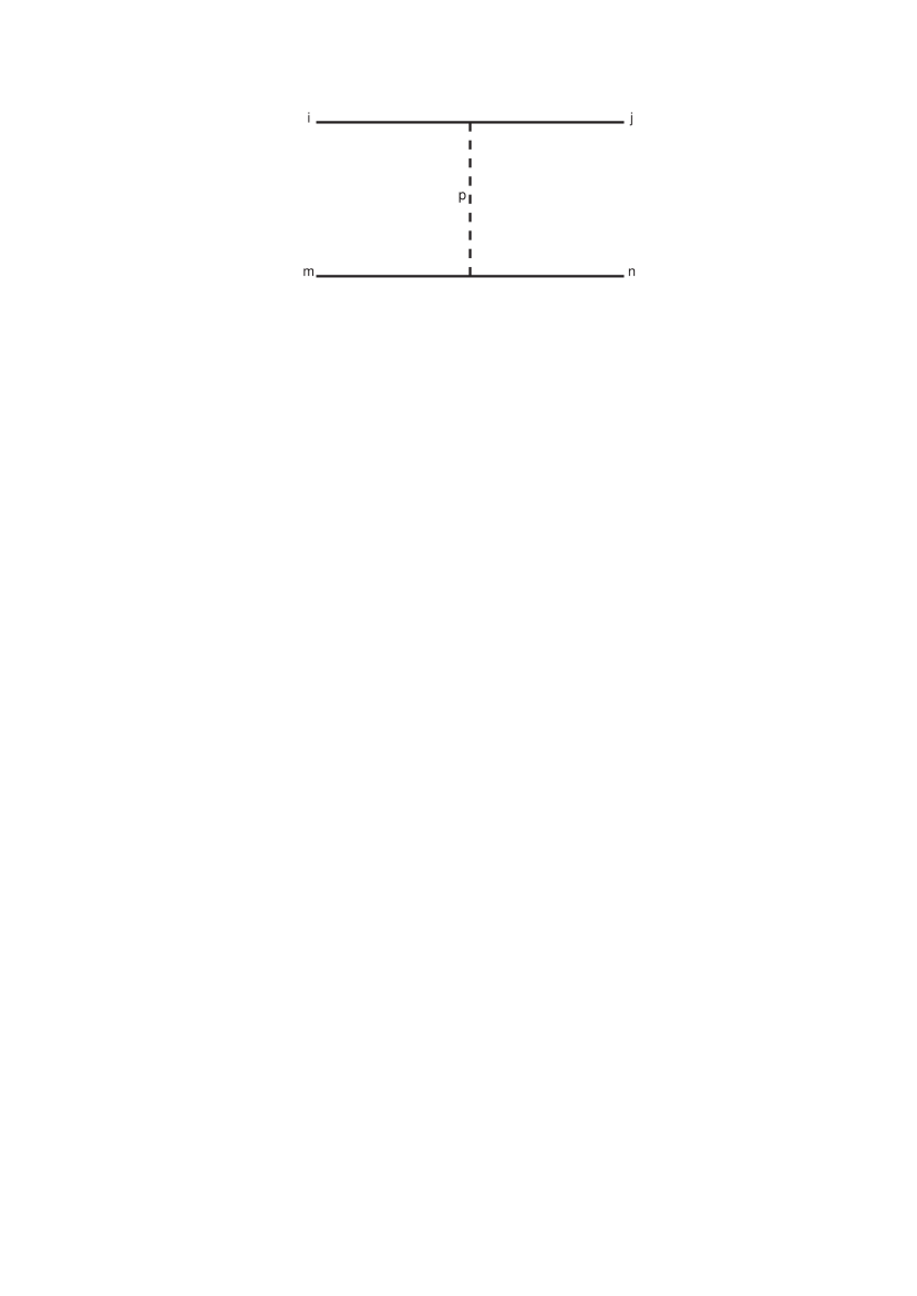
Figure 1: Octet representation indices OBE-graphs. The solid lines denote baryons with labels $i,m,j,n$. The dashed line with label p refers to the bosons: pseudoscalar, vector, axial-vector, or scalar mesons.

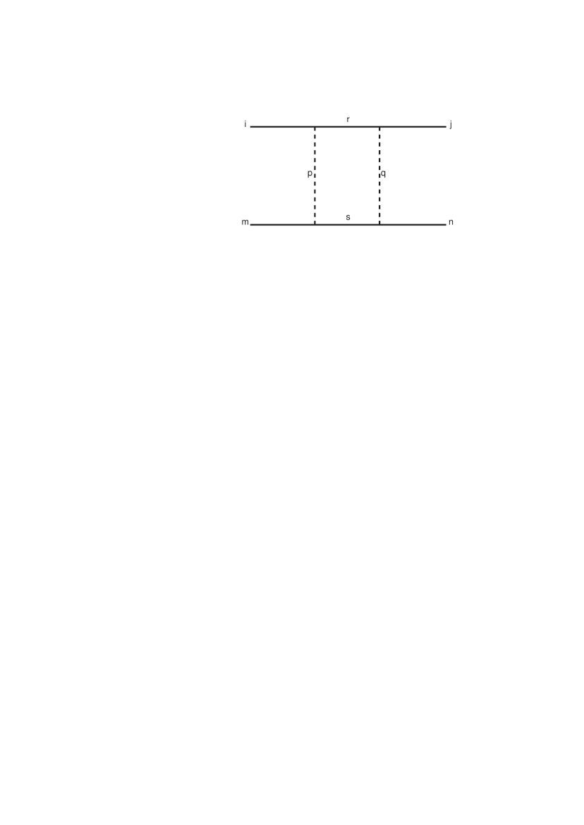
Figure 2: Octet representation indices TME-parallel-graphs. The solid lines denote baryons with labels $i,m,j,n,r,s$. The dashed lines with labels $p,q$ refer to the pseudoscalar mesons.

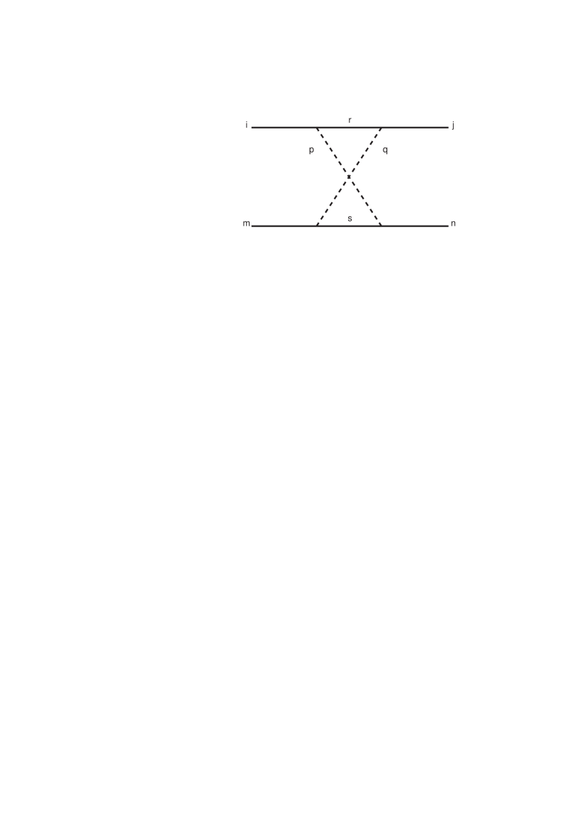
Figure 3: Octet representation indices TME-crossed-graphs. The solid lines denote baryons with labels $i,m,j,n,r,s$. The dashed lines with labels $p,q$ refer to the pseudoscalar mesons.

III MPE interactions and SU(3)

III.1 Pair Couplings and SU(3)-symmetry

Below, $\sigma,{\bf a}_{0},{\bf A}_{1},\ldots$ are short-hands for respectively the nucleon densities $\bar{\psi}\psi$, $\bar{\psi}\mbox{\boldmath$\tau$}\psi$, $\bar{\psi}\gamma_{5}\gamma_{\mu}\mbox{\boldmath$\tau$}\psi,\ldots$.

The SU(3)-octet and -singlet mesons, denoted by the subscript $8$ respectively $1$, are in terms of the physical ones defined as follows:

1. Pseudo-scalar-mesons:

   $$\eta_{1} = \cos\theta_{PV}\eta^{\prime}-\sin\theta_{PV}\eta$$

   $$\eta_{8} = \sin\theta_{PV}\eta^{\prime}+\cos\theta_{PV}\eta$$

   Here, $\eta^{\prime}$ and $\eta$ are the physical pseudoscalar mesons $\eta(957)$ respectively $\eta(548)$.

2. Vector-mesons:

   $$\phi_{1} = \cos\theta_{V}\omega-\sin\theta_{V}\phi$$

   $$\phi_{8} = \sin\theta_{V}\omega+\cos\theta_{V}\phi$$

   Here, $\phi$ and $\omega$ are the physical vector mesons $\phi(1019)$ respectively $\omega(783)$.

Then, one has the following SU(3)-invariant pair-interaction Hamiltonians:
1. SU(3)-singlet couplings $S^{\alpha}_{\beta}=\delta^{\alpha}_{\beta}\sigma/\sqrt{3}$:

$${\cal H}_{S_{1}PP} = \frac{g_{S_{1}PP}}{\sqrt{3}}\left\{\mbox{\boldmath$\pi$}\cdot\mbox{\boldmath$\pi$}+2K^{\dagger}K+\eta_{8}\eta_{8}\right\}\cdot\sigma$$

2. SU(3)-octet symmetric couplings I, $S^{\alpha}_{\beta}=(S_{8})^{\alpha}_{\beta}\Rightarrow(1/4)Tr\{S[P,P]_{+}\}$:

$${\cal H}_{S_{8}PP} = \frac{g_{S_{8}PP}}{\sqrt{6}}\left\{\vphantom{\frac{A}{A}}\right.({\bf a}_{0}\cdot\mbox{\boldmath$\pi$})\eta_{8}+\frac{\sqrt{3}}{2}{\bf a}_{0}\cdot(K^{\dagger}\mbox{\boldmath$\tau$}K)$$

$$+ \frac{\sqrt{3}}{2}\left\{(K_{0}^{\dagger}\mbox{\boldmath$\tau$}K)\cdot\mbox{\boldmath$\pi$}+h.c.\right\}$$

$$- \frac{1}{2}\left\{(K_{0}^{\dagger}K)\eta_{8}+h.c.\right\}$$

$$+ \frac{1}{2}f_{0}\left(\mbox{\boldmath$\pi$}\cdot\mbox{\boldmath$\pi$}-K^{\dagger}K-\eta_{8}\eta_{8}\right)\left.\vphantom{\frac{A}{A}}\right\}$$

3. SU(3)-octet symmetric couplings II, $S^{\alpha}_{\beta}=(B_{8})^{\alpha}_{\beta}\Rightarrow(1/4)Tr\{B^{\mu}[V_{\mu},P]_{+}\}$:

$${\cal H}_{B_{8}VP} = \frac{g_{B_{8}VP}}{\sqrt{6}}\left\{\vphantom{\frac{A}{A}}\right.\frac{1}{2}\left[\left({\bf B}_{1}^{\mu}\cdot\mbox{\boldmath$\rho$}_{\mu}\right)\eta_{8}+\left({\bf B}_{1}^{\mu}\cdot\mbox{\boldmath$\pi$}_{\mu}\right)\phi_{8}\right]$$

$$+ \frac{\sqrt{3}}{4}\left[{\bf B}_{1}\cdot(K^{*\dagger}\mbox{\boldmath$\tau$}K)+h.c.\right]$$

$$+ \frac{\sqrt{3}}{4}\left[(K_{1}^{\dagger}\mbox{\boldmath$\tau$}K^{*})\cdot\mbox{\boldmath$\pi$}+(K_{1}^{\dagger}\mbox{\boldmath$\tau$}K)\cdot\mbox{\boldmath$\rho$}+h.c.\right]$$

$$- \frac{1}{4}\left[(K_{1}^{\dagger}\cdot K^{*})\eta_{8}+(K_{1}^{\dagger}\cdot K)\phi_{8}+h.c.\right]$$

$$+ \frac{1}{2}H^{0}\left[\mbox{\boldmath$\rho$}\cdot\mbox{\boldmath$\pi$}-\frac{1}{2}\left(K^{*\dagger}\cdot K+h.c.\right)-\phi_{8}\eta_{8}\right]\left.\vphantom{\frac{A}{A}}\right\}$$

4. SU(3)-octet a-symmetric couplings I, $A^{\alpha}_{\beta}=(V_{8})^{\alpha}_{\beta}\Rightarrow(-i/\sqrt{2})Tr\{V^{\mu}[P,\partial_{\mu}P]_{-}\}$:

$${\cal H}_{V_{8}PP} = g_{A_{8}PP}\left\{\vphantom{\frac{A}{A}}\right.\frac{1}{2}\mbox{\boldmath$\rho$}_{\mu}\cdot\mbox{\boldmath$\pi$}\times\stackrel{{\scriptstyle\leftrightarrow}}{{\partial^{\mu}}}\!\!\mbox{\boldmath$\pi$}+\frac{i}{2}\mbox{\boldmath$\rho$}_{\mu}\cdot(K^{\dagger}\mbox{\boldmath$\tau$}\!\!\stackrel{{\scriptstyle\leftrightarrow}}{{\partial^{\mu}}}\!\!K)$$

$$+ \frac{i}{2}\left(\vphantom{\frac{A}{A}}K^{*\dagger}_{\mu}\mbox{\boldmath$\tau$}(K\!\!\stackrel{{\scriptstyle\leftrightarrow}}{{\partial^{\mu}}}\!\!\mbox{\boldmath$\pi$})-h.c.\right)+i\frac{\sqrt{3}}{2}\left(\vphantom{\frac{A}{A}}K^{*\dagger}_{\mu}\cdot\right.$$

$$\left.(K\cdot\stackrel{{\scriptstyle\leftrightarrow}}{{\partial^{\mu}}}\!\!\eta_{8})-h.c.\vphantom{\frac{A}{A}}\right)+\frac{i}{2}\sqrt{3}\phi_{\mu}(K^{\dagger}\stackrel{{\scriptstyle\leftrightarrow}}{{\partial^{\mu}}}\!\!K)\left.\vphantom{\frac{A}{A}}\right\}$$

5. SU(3)-octet a-symmetric couplings II, $A^{\alpha}_{\beta}=(A_{8})^{\alpha}_{\beta}\Rightarrow(-i/\sqrt{2})Tr\{A^{\mu}[P,V_{\mu}]_{-}\}$:

$${\cal H}_{A_{8}VP} = g_{A_{8}VP}\left\{\vphantom{\frac{A}{A}}\right.{\bf A}_{1}\cdot\mbox{\boldmath$\pi$}\times\mbox{\boldmath$\rho$}$$

$$+ \frac{i}{2}{\bf A}_{1}\cdot\left[(K^{\dagger}\mbox{\boldmath$\tau$}K^{*})-(K^{*\dagger}\mbox{\boldmath$\tau$}K)\right]$$

$$- \frac{i}{2}\left(\left[(K^{\dagger}\mbox{\boldmath$\tau$}K_{A})\cdot\mbox{\boldmath$\rho$}+(K_{A}^{\dagger}\mbox{\boldmath$\tau$}K^{*})\cdot\mbox{\boldmath$\pi$}\right]-h.c.\right)$$

$$- i\frac{\sqrt{3}}{2}\left(\left[(K^{\dagger}\cdot K_{A})\phi_{8}+(K_{A}^{\dagger}\cdot K^{*})\eta_{8}\right]-h.c.\right)$$

$$+ \frac{i}{2}\sqrt{3}f_{1}\left[K^{\dagger}\cdot K^{*}-K^{*\dagger}\cdot K\right]\left.\vphantom{\frac{A}{A}}\right\}$$

The relation with the pair-couplings of RS96ab and paper I is $g_{S_{1}PP}/\sqrt{3}=g_{(\pi\pi)_{0}}/m_{\pi}$, $g_{A_{8}VP}=g_{(\pi\rho)_{1}}/m_{\pi}$ etc.

III.2 Computations MPE-graphs SU(3)-factors

The SU(3) matrix elements for the graphs with meson-pair vertices, the so-called MPE-graphs Fig. 4 and Fig. 5 are, using the cartesian-octet representation in section II.3, given by

$$M_{(1-pair)}(j,n;i,m) = \sum_{p,q,r,s}^{\prime}H_{pair}(j,i,s)\ O(q,p,s)$$ (36)

$$\times H_{2}(m,r,q)\ H_{1}(r,m,p)$$

$$M_{(2-pair)}(j,n;i,m) = \sum_{p,q,r,s=1}^{\prime}H_{pair}(j,i,s)\ O(q,p,s)$$ (37)

$$\times O(q,p,r)\ H_{pair}(n,m,p)$$

Again, like in the OBE-case, the numerical values of the SU(3) matrix elements for MPE can be computed straightforwardly making a computer program.

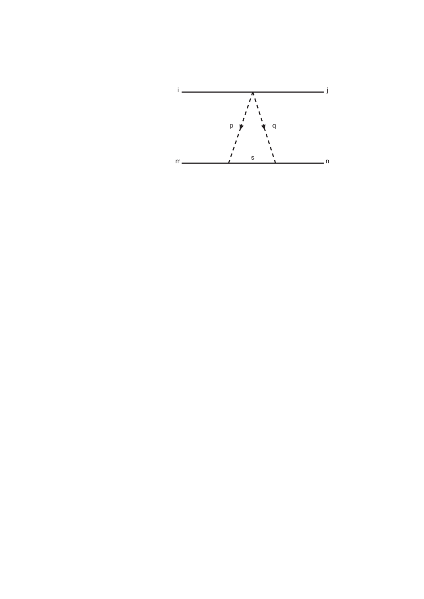
Figure 4: Octet representation indices MPE one-pair-graphs. The solid lines denote baryons with labels $i,m,j,n,s$. The dashed lines with labels $p,q$ refer to the pseudoscalar etc. mesons.

Figure 5: Octet representation indices MPE two-pair-graphs. The solid lines denote baryons with labels $i,m,j,n$. The dashed lines with labels $p,q$ refer to the pseudoscalar etc. mesons.

IV Broken SU(3)-Couplings and Form Factors

IV.1 Broken SU(3) BBM-couplings

In our models, breaking of the SU(3) symmetry is introduced in several places. First of all, we use the physical masses for the baryons and mesons. Second, we allow for the fact that the $\Lambda$ and $\Sigma^{0}$ have the same quark content, and so there is an appreciable mixing between the isospin-pure $\Lambda$ and $\Sigma^{0}$ states Dal64 . Although exact ${\rm SU}(2)\subset{\rm SU}(3)$ symmetry requires that $f_{\Lambda\Lambda\pi^{0}}=0$, $\Lambda$-$\Sigma^{0}$ mixing and the interaction $\Sigma^{0}\rightarrow\Lambda+\pi^{0}$ result in a non-zero coupling constant for the physical $\Lambda$-hyperon, derived by Dalitz and von Hippel Dal64 . This $\Lambda-\Sigma^{0}$-mixing leads also to a non-zero coupling of the $\Lambda$ to the other $I=1$ mesons: $\rho(760),a_{0}(980),a_{1}(1270)$, as well as to the $I=1$-pairs. For the details of these OBE-couplings see e.g. RSY99 , equations (2.15)-(2.17). The corresponding so-called CSB-potentials are included in the ESC-model for OBE, TME, and MPE.

In paper I of this series we have shown that the NNM-coupling constants are described pretty well by the ${}^{3}P_{0}$ mechanism Mic69 ; LeY73 ; Cha80 . In this paper we use the predictions of the ${}^{3}P_{0}$-model for the $F/(F+D)$-ratios as well. Therefore, it is most natural to use for the description of a possible flavor symmetry breaking of the coupling constants the ${}^{3}P_{0}$ mechanism as well, like in RSY99 . In RSY99 it is argued that a symmetric treatment of the ‘moving’-quarks and the pair-quarks in the ${}^{3}P_{0}$-coupling process is appropriate, since this leads to a covariant vertex. Therefore, in RSY99 the ${}^{3}P_{0}$-Hamiltonian for the $BBM$-couplings is taken as follows

$$H_{I}=\int d^{3}x\int d^{3}y\ F(x-y)\cdot$$

$$\times\left[\bar{q}(x)O_{\bar{q}q}q(x)\right]^{(1)}\otimes\left[\bar{q}(y)O_{\bar{q}q}q(y)\right]^{(2)}$$ (38)

where the quark-field operators are vectors in flavor-space, with components $q_{i}=(u,d,s)$ and $\bar{q}_{i}=(\bar{u},\bar{d},\bar{s})$. (In the following we will refer to the non-strange quarks $u$ and $d$ as $n$-quarks.) It is understood in (38) that the first factor creates or annihilates a quark-pair, whereas the second factor ‘moves’ a quark from the baryon into the meson or vice versa. O is a matrix in quark-flavor space, which, supposing no quark-mixing, is diagonal. However since it will in general break SU(3)- and SU(2)-symmetry by using the form

$$(O_{\bar{q}q})_{i,j}=\left(\begin{array}[]{ccc}\gamma_{u}&0&0\\ 0&\gamma_{d}&0\\ 0&0&\gamma_{s}\end{array}\right)\ ,\\$$ (39)

where the pair-creation constants $\gamma_{u},\gamma_{d}$, and $\gamma_{s}$ in principle could be unequal. The CSB described above is on the quark-level due to $\gamma_{u}\neq\gamma_{d}$. For a more detailed description of some properties of the Hamiltonian in (38) and $(O_{\bar{q}q})_{i,j}$ we refer to RSY99 .

Here, we assume that there is, also ’flavor-symmetry-breaking’ (FSB) of the ’medium strong’ kind, i.e. $\gamma_{n}=\gamma_{u}=\gamma_{d}\neq\gamma_{s}$. We introduce this medium strong SU(3)-breaking according to the ${}^{3}P_{0}$-model by a modification of the $s\bar{s}$-coupling, using the ratio $\Delta_{FSB}=\gamma_{s}/\gamma_{n}-1$. For $\Delta_{FSB}=0$ there is no SU(3)-breaking, while for $\Delta_{FSB}\neq 0$ there is.

The $I=1$-meson couplings for NN are determined in the process of NN-fitting. This fixes $\gamma_{n}$. In the coupling of the $I=1/2$-mesons, $K,K^{*},\kappa$, , only one $s\bar{s}$-operator is active and the SU(3)-breaking of the coupling is given by

$$\Delta g_{\Lambda NK} = \Delta_{FSB}\ \hat{g}_{\Lambda NK}\ ,\$$ (40)

and completely similar expressions for $\Delta g_{\Sigma NK}$, $\Delta g_{\Xi\Lambda K}$, and $\Delta g_{\Xi\Sigma K}$. Here, $\hat{g}_{\Lambda NK}$ etc. are calculated as usual in terms of $g_{NN\pi}$ and the SU$(3)$-scheme with $\alpha_{PV}$. Similar formulas we used for the SU(3)-breaking in the case of the vector, axial-vector, and scalar mesons.

In the case of the $I=0$-mesons two $s\bar{s}$-operators are active in the baryon-baryon coupling. Now, the $I=0$-mesons have a $n\bar{n}$- and a $s\bar{s}$- component. In our scheme only the coupling of the $s\bar{s}$ is affected by the SU(3)-breaking. Therefore, it is natural to transform first to the so-called ’ideal’ $q\bar{q}$-basis, applying the SU(3)-breaking, and transform back to the physical basis. This scheme is as follows:

1. The $I=0$ $|n\bar{n}\rangle=|u\bar{u}+d\bar{d}\rangle/\sqrt{2}$- and the $-|s\bar{s}\rangle$-states are in $SU(3)$ linear combinations of the $\{1\}$ and $\{8\}$-octet states. Likewise, the coupling of the $n\bar{n}$- and $s\bar{s}$-quark pairs to baryons are the same linear combinations, i.e.

   $$\hat{g}_{n\bar{n}} = \cos\theta_{I}\ \hat{g}_{1}+\sin\theta_{I}\ \hat{g}_{8}\ ,$$

   $$\hat{g}_{s\bar{s}} = -\sin\theta_{I}\ \hat{g}_{1}+\cos\theta_{I}\ \hat{g}_{8}\ ,$$ (41)

   where $\cos\theta_{I}=\sqrt{2/3}$, and $\sin\theta_{I}=\sqrt{1/3}$.

2. Since for the $s\bar{s}$-coupling process two strange quark pairs are involved, and none in the $n\bar{n}$-coupling, the FSB is given on the level of the quark-pair coupling by:

   $$g_{n\bar{n}}\rightarrow\hat{g}_{n\bar{n}}\ \ ,\ \ g_{s\bar{s}}\rightarrow\left(1+\Delta_{FSB}\right)^{2}\hat{g}_{s\bar{s}}\ .$$ (42)

3. The translation of this breaking to the level of the $\{1\}$ and $\{8\}$-octet couplings is the inverse transformation of (41), and from there to the physical mesons. For example in the case of the vector mesons we have

   $$g_{\omega} = \cos\Delta\theta_{V}\ g^{V}_{1}+\sin\Delta\theta_{V}\ g^{V}_{8}\ ,$$

   $$g_{\phi} = -\sin\Delta\theta_{V}\ g^{V}_{1}+\cos\Delta\theta_{V}\ g^{V}_{8}\ ,$$ (43)

   where $\Delta\theta_{V}=\theta_{V}-\theta_{I}$. The similar procedure is used for the pseudoscalar, scalar, and axial-vector mesons.

This breaking applies to the NNM-, YNM-, and YYM-couplings, containing the free parameter $\Delta_{PS}$ for the pseudoscalar mesons, and one parameter $\Delta_{V}$ which is used for the vector, axial-vector, and scalar mesons.

We note that this breaking somewhat differs from that used in NSC97 RSY99 , which was based on an SU(6)_W-scheme. The problem with the latter, from our viewpoint is, that the states of for example the vector nonet are a mixture of $W=0$ and $W=1$, making the implementation of SU(3)-breaking less straightforward as in the scheme described above.

The implementation of this scheme in practice is done as follows. We start, for example in the case of the vector mesons for the g-couplings, with the parameter set $(\hat{g}_{\rho},\hat{g}_{\omega},\theta_{V},\alpha_{V})$ and compute all couplings in the usual SU(3)-scheme, giving $\hat{g}_{NN\rho},\hat{g}_{\Sigma\Sigma\rho}$, etc. This defines the singlet $\{1\}$ couplings

$$\hat{g}_{1} = \left[\hat{g}_{\omega}-\sin\theta_{V}\hat{g}_{8}\right]/\cos\theta_{V}\ ,$$

where the octet $\{8\}$ coupling for nucleons is given by $\hat{g}_{8}=(4\alpha_{V}-1)\hat{g}_{NN\rho}/\sqrt{3}$, and similarly for $\Lambda$, $\Sigma$, and $\Xi$. Then, we compute $\hat{g}_{n\bar{n}}$ and $\hat{g}_{s\bar{s}}$ using (41). Subsequently we compute the symmetry breaking by the transformation etc. as described above, and finally we compute the coupling constants $g_{\omega},g_{\phi}$, etc.

We finish this discussion by noticing that for the $I=1$-mesons $\pi,\rho,a_{0},a_{1}$ for all baryon couplings $g=\hat{g}$, because then only n-quarks are ’active’.

IV.2 Form Factors

Also in this work, like in the NSC97-models RSY99 , the form factors depend on the SU(3) assignment of the mesons, In principle, we introduce form factor masses $\Lambda_{8}$ and $\Lambda_{1}$ for the $\{8\}$ and $\{1\}$ members of each meson nonet, respectively. In the application to ${\it YN}$ and ${\it YY}$, we allow for SU(3)-breaking, by using different cut-offs for the strange mesons $K$, $K^{*}$, and $\kappa$. Moreover, for the $I=0$-mesons we assign the cut-offs as if there were no meson-mixing. For example we assign $\Lambda_{1}$ for $\eta^{\prime},\omega,\epsilon$, and $\Lambda_{8}$ for $\eta,\phi,S^{*}$, etc. For the axial-mesons we use a single cut-off $\Lambda^{A}$.

V ESC04-model: Fitting ${\it NN}\oplus{\it YN}$-data

Like in the NN-fit, described in I, also in the simultaneous $\chi^{2}$-fit of the NN- and YN-data, it appeared again that the OBE-couplings could be constraint successfully by the ’naive’ predictions of the QPC-model LeY73 . Although these predictions, see I, section IV, are ’bare’ ones, we tried to keep during the searches many OBE-couplings rather closely in the neighborhood of the predicted values. Also, it appeared that we could either fix the $F/(F+D)$-ratios to those as suggested by the QPC-model, or apply the same restraining strategy as for the OBE-couplings.

In the simultaneous $\chi^{2}$-fit of the NN- and YN-data a single set of parameters was used. Of course, it is to be expected that the accurate and very numerous NN-data essentially fix most of the parameters. Only some of the parameters, for example certain $F/(F+D)$-ratios, are influenced by the YN-data.

V.1 Parameters and Nucleon-nucleon Fit

For the cut-off masses $\Lambda$ we used as free parameters $\Lambda_{8}^{P},\Lambda_{8}^{V},\Lambda_{1}^{V}$, and $\Lambda^{A}$. The $I=0$ cut-off masses for the pseudoscalar and scalar mesons were fixed to $\Lambda_{1}^{P}=900$ MeV, and $\Lambda_{1}^{S}\approx 1100$ MeV.

The treatment of the broad mesons $\rho$ and $\epsilon$ is similar to that in the OBE-models NRS78 ; MRS89 . For the $\rho$-meson the same parameters are used as in these references. However, for the $\epsilon=f_{0}(760)$ assuming $m_{\epsilon}=760$ MeV and $\Gamma_{\epsilon}=640$ MeV the Bryan-Gersten parameters Bry72 are used. For the chosen mass and width they are: $m_{1}=496.39796$ MeV, $m_{2}=1365.59411$ MeV, and $\beta_{1}=0.21781,\beta_{2}=0.78219$. The ’mass’ of the diffractive exchanges were all fixed to $m_{P}=309.1$ MeV.

Summarizing the parameters we have for NN:

1. QPC-constrained: $g_{NN\rho},g_{NN\omega}$,
   $f_{NN\rho},f_{NN\omega},f_{NNa_{1}},g_{a_{0}},g_{NN\epsilon},g_{NNA_{2}},g_{NNP}$,

2. Pair couplings: $g_{NN(\pi\pi)_{1}},f_{NN(\pi\pi)_{1}},g_{NN(\pi\rho)_{1}}$,
   $g_{NN\pi\omega},g_{NN\pi\eta},g_{NN\pi\epsilon}$,

3. Cut-off masses: $\Lambda_{8}^{P},\Lambda_{8}^{V},\Lambda_{8}^{S},\Lambda_{1}^{V},\Lambda^{A}$.

Of course, also the couplings for the pseud-scalar mesons $f_{NN\pi},f_{NN\eta^{\prime}}$ were fitted. The pair coupling $g_{NN(\pi\pi)_{0}}$ was kept fixed at a small, but otherwise arbitrary value.

The NN-data used are the same as in I, and we refer the reader to this paper for a description of the employed phase shift analysis Sto93 ; Klo93 . Differences with I are that here we did not fit the NN-low energy parameters and the deuteron binding energy explicitly.

V.2 Parameters and Hyperon-nucleon Fit

All ’best’ low-energy YN-data are included in the fitting, This is a selected set of 35 low-energy Y​N-data, the same set has been used in MRS89 and RSY99 . We added 3 (preliminary) total $\Sigma^{+}p$ X-sections from the recent KEK-experiment E289 Kanda05 . In section VIII these are given together with the results. Next to these we added ’pseudo-data’ for the $\Lambda p$ and $\Lambda\Lambda$ scattering length’s and effective ranges, in fm:

$$\hat{a}_{\Lambda p}(^{1}S_{0}) = -1.95\pm 0.10\ \ ,\ \ \hat{r}_{\Lambda p}(^{1}S_{0})=2.90\ ,$$

$$\hat{a}_{\Lambda p}(^{3}S_{1}) = -1.86\pm 0.10\ \ ,\ \ \hat{r}_{\Lambda p}(^{1}S_{0})=2.70\ ,$$

$$\hat{a}_{\Lambda\Lambda}(^{1}S_{0}) = -3.00\pm 0.10\ ,$$ (44)

The $\Lambda p$-values which are suggested by the experience in several hyper-nuclear applications of the NSC97-models. Also, during the fitting checks were done to prevent the occurrence of bound states. Parameters, typically strongly influenced by the YN-data, are

1. $F/(F+D)$-parameters: $\alpha_{PV}$, $\alpha_{V}^{m}$, $\alpha_{S}$,

2. SU(3)-symmetry breaking: $\Delta_{FSB}$.

Notice that the strange octet-mesons $K$ etc. were given the same form factors as their non-strange companions. So, because of YN we have introduced 4 extra free parameters. We notice that the need to avoid bound states in the YN and YY systems has in particularly some influence on the trio $g_{\epsilon},g_{\omega}$, and $g_{P}$. Of particular importance of this was the introduction of the zero in the scalar-meson form factors, see paper I for a detailed description. Like in I, also here we used a fixed zero by taking $U=750$ MeV.

VI Coupling Constants, $F/(F+D)$ Ratios, and Mixing Angles

Like in paper I, we constrained the OBE-couplings by the ’naive’ predictions of the QPC-model Mic69 . We kept during the searches all OBE-couplings in the neighborhood of these predictions, but a little less so than in paper I. The same has been done for all $\alpha=F/(F+D)$-ratios, i.e. for BBM- and the BB-Pair-couplings. In fact, all $F/(F+D)$-ratios were fixed, except the ratio $\alpha_{V}^{m}$ for vector mesons and $\alpha_{S}$ for the scalar mesons.

The mixing for the pseudoscalar, vector, and scalar mesons, as well as the handling of the diffractive potentials, has been described elsewhere, see e.g. MRS89 ; RSY99 . The mixing etc. of the axial-vector mesons is completely the same as for the vector etc. mesons, and also need not be discussed here.

In Table 3 we give the fitted ESC04 meson couplings and parameters.

Table 3: Meson couplings and parameters employed in the ESC04-potentials. Coupling constants are at ${\bf k}^{2}=0$. An asterisk denotes that the coupling constant is not searched, but constrained via SU(3) are simply put to some value used in previous work. The used widths of the $\rho$ and $\varepsilon$ are 146 MeV and 640 MeV respectively.

meson	mass (MeV)	$g/\sqrt{4\pi}$	$f/\sqrt{4\pi}$	$\Lambda$ (MeV)
$\pi$	138.04		0.2631	833.63
$\eta$	548.80		0.1933∗	,,
$\eta^{\prime}$	957.50		0.1191	900.00
$\rho$	770.00	0.7800	3.4711	839.53
$\phi$	1019.50	–0.3788	–0.0494∗	,,
$\omega$	783.90	3.0138	0.4467	869.84
$a_{1}$	1270.00	2.5426		945.66
$f_{1}$	1420.00	0.8896∗		,,
$f_{1}^{\prime}$	1285.00	1.2544		,,
$a_{0}$	962.00	0.9251		1159.88
$f_{0}$	993.00	–0.8162		,,
$\varepsilon$	760.00	3.4635		1101.61
$a_{2}$	309.10	0.0000
$f_{2}$	309.10	0.0000
$f_{2}^{\prime}$	309.10	0.0000
Pomeron	309.10	1.9651

In Table 4 we compare the fitted meson coupling constants with the ’naive’ predictions of the QPC-model. For the QPC-predictions in Table 4, see paper I. One sees that the fitted parameters are rather close to those of the QPC-model, and even more so than in paper I. Notice that we omitted here the pion coupling, which requires a different $\gamma_{M}$ factor in the QPC-model, see remarks in I. Also, we see that the deviation between the scalar and vector couplings from the QPC-model relations, $g_{\epsilon}-g_{\omega}\approx 3(g_{a_{0}}-g_{\rho})$, which seems a purely isospin factor.

Table 4: NN+YN: ESC04 Couplings and ${}^{3}P_{0}$-Model Relations.

Meson	$r_{M}[{\rm fm]}$	$X_{M}$	$\gamma_{M}$	${}^{3}P_{0}$	ESC04
$\rho(770)$	0.56	$1/2$	1.53	$g=0.78$	$g=0.78$
$\omega(783)$	0.56	$3/2$	1.53	$g=2.40$	$g=3.01$
$a_{0}(962)$	0.56	$\sqrt{3}/2$	1.53	$g=0.79$	$g=0.92$
$\epsilon(760)$	0.56	$3\sqrt{3}/2$	1.53	$g=2.11$	$g=3.46$
$a_{1}(1270)$	0.56	$3\sqrt{3}/2$	1.53	$g=2.73$	$g=2.54$

In Table 5 the SU(3) singlet and octet couplings are listed i.e. $\hat{g}$ etc., and also $F/(F+D)$-ratios and mixing angles.

Table 5: Coupling constants, $F/(F+D)$-ratio’s, mixing angles etc. The values with $\star)$ have been determined in the fit to the YN-data. The other parameters are theoretical input or determined by the fitted parameters and the constraint from the NN-analysis.

mesons		$\{1\}$	$\{8\}$	$F/(F+D)$	angles
ps-scalar	f	0.1852	0.2631	$\alpha_{PV}=0.4668^{\star)}$	$\theta_{P}=-23.00^{0}$
vector	g	2.6218	0.7800	$\alpha^{e}_{V}=1.0$	$\theta_{V}=37.50^{0}$
	f	0.3845	3.4711	$\alpha^{m}_{V}=0.2760^{\star)}$
axial	g	1.5023	2.5426	$\alpha_{A}=0.2340$	$\theta_{A}=-23.00^{0~{}\star)}$
scalar	g	3.1688	0.9251	$\alpha_{S}=0.8410$	$\theta_{S}=40.32^{0~{}\star)}$
diffractive	g	1.9651	0.0000	$\alpha_{D}=1.000$	$\psi_{D}=0.0^{0~{}\star)}$

In Table 6 and in Table 7 we list the couplings of the physical mesons to the nucleons $(Y=1)$, and the hyperons with $Y=0$. These were computed using the FSB-scheme, described above. We found (ESC04a) $\Delta_{FSB}(PV)=-0.258$, and $\Delta_{FSB}(V,S,A)=-0.267$.

Table 6: Coupling constants for pseudoscalar and vector meson $Y=0$ and $Y=\pm 1$ exchanges.

M		NNM	$\Lambda\Lambda M$	$\Lambda\Sigma M$	$\Sigma\Sigma M$	$\Lambda NM$	$\Sigma NM$
$\pi$	g	3.57602	CSB	2.47895	4.23203	—	—
	f	0.26306	CSB	0.16196	0.24559	—	—
$\eta$	f	0.19333	–0.02028	—	0.21534	—	—
$\eta^{{}^{\prime}}$	f	0.11908	0.14213	—	0.11671	—	—
$K$	g	—	—	—	—	–3.22933	0.19837
	f	—	—	—	—	–0.21786	0.01296
$\rho$	g	0.78000	CSB	—	1.56000	—	—
	f	3.47113	CSB	2.90094	1.91768	—	—
$\phi$	g	–0.37884	–0.94125	—	–0.94125	—	—
	f	–0.04944	–1.34461	—	1.07066	—	—
$\omega$	g	3.01376	2.21121	—	2.21121	—	—
	f	0.44671	–1.40149	—	2.04507	—	—
$K^{\star}$	g	—	—	—	—	–0.99079	–0.57203
	f	—	—	—	—	–2.28171	1.13927
$a_{1}$	g	2.54264	CSB	2.24770	1.19215	—	—
$f_{1}$	g	0.88961	–0.66726	—	2.57849	—	—
$f^{\prime}_{1}$	g	1.25438	1.40489	—	1.09111	—	—
$K_{1}$	g	—	—	—	—	–1.58137	0.99042

Table 7: Coupling constants for scalar meson and ‘diffractive’ $Y=0$ and $Y=\pm 1$ exchanges. Nomenclature scalar mesons: $\delta=a_{0}(962)$, $\epsilon=f_{0}(760)$, $S^{*}=f_{0}(993)$, $\kappa=K_{0}^{*}(900)$.

M		NNM	$\Lambda\Lambda M$	$\Lambda\Sigma M$	$\Sigma\Sigma M$	$\Lambda NM$	$\Sigma NM$
$\delta$	g	0.92511	CSB	0.16975	1.55621	—	—
$S^{*}$	g	–0.81620	–1.36993	—	–1.23870	—	—
$\epsilon$	g	3.46354	2.58418	—	2.79258	—	—
$\kappa$	g	—	—	—	—	–1.05063	–0.46283
$A_{2}$	g	0.00000	CSB	0.00000	0.00000	—	—
$P$	g	1.96510	1.96510	—	1.96510	—	—
$K^{\star\star}_{2}$	g	—	—	—	—	0.00000	0.00000

In Table 8 we listed the fitted Pair-couplings for the MPE-potentials. We recall that only One-pair graphs are included, in order to avoid double counting, see paper I. The $F/(F+D)$-ratios are all fixed, assuming heavy-boson domination of the pair-vertices. The ratios are taken from the QPC-model for $Q\bar{Q}$-systems with the same quantum numbers as the dominating boson. The BB-Pair couplings are computed, assuming unbroken SU(3)-symmetry, from the NN-Pair coupling and the $F/(F+D)$-ratio using SU(3).

Table 8: Pair-meson coupling constants employed in the ESC04 MPE-potentials. Coupling constants are at ${\bf k}^{2}=0$.

$J^{PC}$	SU(3)-irrep	$(\alpha\beta)$	$g/4\pi$	$F/(F+D)$
$0^{++}$	$\{1\}$	$g(\pi\pi)_{0}$	—	—
$0^{++}$	,,	$g(\sigma\sigma)$	—	—
$0^{++}$	$\{8\}_{s}$	$g(\pi\eta)$	–0.1860	1.000
$1^{--}$	$\{8\}_{a}$	$g(\pi\pi)_{1}$	–0.0024	1.000
		$f(\pi\pi)_{1}$	0.1310	0.400
$1^{++}$	,,	$g(\pi\rho)_{1}$	0.8864	0.643
$1^{++}$	,,	$g(\pi\sigma)$	–0.0241	0.643
$1^{++}$	,,	$g(\pi P)$	0.0	—
$1^{+-}$	$\{8\}_{s}$	$g(\pi\omega)$	–0.1722	0.467

Unlike in RS96ab , we did not fix pair couplings using a theoretical model, based on heavy-meson saturation and chiral-symmetry. So, in addition to the 14 parameters used in RS96ab we now have 6 pair-coupling fit parameters. In Table 8 the fitted pair-couplings are given. Note that the $(\pi\pi)_{0}$-pair coupling gets contributions from the $\{1\}$ and the $\{8_{s}\}$ pairs as well, giving in total $g_{(\pi\pi)}=0.10$, which has the same sign as in RS96ab . The $f_{(\pi\pi)_{1}}$-pair coupling has opposite sign as compared to RS96ab . In a model with a more complex and realistic meson-dynamics SR97 this coupling is predicted as found in the present ESC-fit. The $(\pi\rho)_{1}$-coupling agrees nicely with $A_{1}$-saturation, see RS96ab . We conclude that the pair-couplings are in general not well understood, and deserve more study.

In the ESC-model described here, is fully consistent with SU(3)-symmetry using a straightforward extension of the NN-model to YN and YY. For example $g_{(\pi\rho)_{1}}=g_{A_{8}VP}$, and besides $(\pi\rho)$-pairs one sees also that $KK^{*}(I=1)$- and $KK^{*}(I=0)$-pairs contribute to the NN potentials. All $F/(F+D)$-ratio’s are taken fixed with heavy-meson saturation in mind. The approximation we have made in this paper is to neglect the baryon mass differences, i.e. we put $m_{\Lambda}=m_{\Sigma}=m_{N}$. This because we have not yet worked out the formulas for the inclusion of these mass differences, which is straightforward in principle.

VII ESC04-model , $N\!N$-Results

VII.1 Parameters and Nucleon-nucleon Fit

For a more detailed discussion on the NN-fitting we refer to I. Here, we fit only to the 1993 Nijmegen representation of the $\chi^{2}$-hypersurface of the NN scattering data below $T_{\rm lab}=350$ MeV Sto93 ; Klo93 . This in contrast to I where also low-energy parameters are fitted for np and nn. In this simultaneous fit of NN and YN, we obtained for the phase shifts a $\chi^{2}/Ndata=1.22$. In Table 3 the meson parameters are given for the ESC04a-model. In Table 9 the distribution of the $\chi^{2}$ is shown for the ten energy bins, which can be compared with a similar table in paper I. Also, for a comparison with paper I, and for use of this model for the description of NN, we give in Tables 10 and 11 the nuclear-bar phases for pp in case $I=1$, and for np in case $I=0$. The deuteron was not fitted, and we have for the binding energy $E_{B}=2.224797$MeV, which is very close to the $E_{B}(experiment)=2.224644$.

Table 9: $\chi^{2}$ and $\chi^{2}$ per datum at the ten energy bins for the Nijmegen93 Partial-Wave-Analysis. $N_{\rm data}$ lists the number of data within each energy bin. The bottom line gives the results for the total $0-350$ MeV interval. The $\chi^{2}$-access for the ESC04-model in the ${\it NN}+{\it YN}$-fit is denoted by $\Delta\chi^{2}$ and $\Delta\hat{\chi}^{2}$, respectively.

$T_{\rm lab}$	$\sharp$ data	$\chi_{0}^{2}$	$\Delta\chi^{2}$	$\hat{\chi}_{0}^{2}$	$\Delta\hat{\chi}^{2}$
0.383	144	137.5549	22.9	0.960	0.159
1	68	38.0187	53.2	0.560	0.783
5	103	82.2257	7.1	0.800	0.068
10	209	257.9946	53.1	1.234	0.183
25	352	272.1971	62.5	0.773	0.177
50	572	547.6727	240.3	0.957	0.420
100	399	382.4493	73.6	0.959	0.184
150	676	673.0548	104.4	0.996	0.154
215	756	754.5248	214.4	0.998	0.284
320	954	945.3772	333.1	0.991	0.349
Total	4233	4091.122	1164.6	0.948	0.268

Table 10: ESC04 pp and np nuclear-bar phase shifts in degrees.

$T_{\rm lab}$	0.38	1	5	10	25
$\sharp$ data	144	68	103	290	352
$\Delta\chi^{2}$	24	53	7	53	62
${}^{1}S_{0}$	14.62	32.62	54.71	55.07	48.39
${}^{3}S_{1}$	159.39	147.77	118.23	102.70	80.78
$\epsilon_{1}$	0.03	0.11	0.66	1.13	1.71
${}^{3}P_{0}$	0.02	0.13	1.56	3.69	8.58
${}^{3}P_{1}$	-0.01	-0.08	-0.87	-2.01	-4.85
${}^{1}P_{1}$	-0.05	-0.19	-1.52	-3.12	-6.46
${}^{3}P_{2}$	0.00	0.01	0.21	0.64	2.44
$\epsilon_{2}$	-0.00	-0.00	-0.05	-0.19	-0.79
${}^{3}D_{1}$	0.00	-0.01	-0.19	-0.69	-2.85
${}^{3}D_{2}$	0.00	0.01	0.22	0.85	3.72
${}^{1}D_{2}$	0.00	0.00	0.04	0.16	0.67
${}^{3}D_{3}$	0.00	0.00	0.00	0.00	0.01
$\epsilon_{3}$	0.00	0.00	0.01	0.08	0.56
${}^{3}F_{2}$	0.00	0.00	0.00	0.01	0.10
${}^{3}F_{3}$	0.00	0.00	-0.00	-0.03	-0.22
${}^{1}F_{3}$	0.00	0.00	-0.01	-0.07	-0.42
${}^{3}F_{4}$	0.00	0.00	0.00	0.00	0.02
$\epsilon_{4}$	0.00	0.00	0.00	-0.00	-0.05

Table 11: ESC04 pp and np nuclear-bar phase shifts in degrees.

$T_{\rm lab}$	50	100	150	215	320
$\sharp$ data	572	399	676	756	954
$\Delta\chi^{2}$	240	74	104	214	333
${}^{1}S_{0}$	38.40	24.05	13.51	2.79	–10.60
${}^{3}S_{1}$	63.01	43.67	31.44	19.93	6.42
$\epsilon_{1}$	1.94	2.18	2.56	3.22	4.57
${}^{3}P_{0}$	11.65	9.84	5.19	-1.31	-10.86
${}^{3}P_{1}$	-8.23	-13.19	-17.25	-21.85	-28.09
${}^{1}P_{1}$	-9.75	-14.12	-17.78	-22.09	-28.12
${}^{3}P_{2}$	5.75	11.02	14.21	16.29	16.96
$\epsilon_{2}$	-1.68	-2.68	-2.97	-2.83	-2.17
${}^{3}D_{1}$	-6.58	-12.61	-17.06	-21.36	-26.14
${}^{3}D_{2}$	8.92	17.08	21.90	24.70	24.83
${}^{1}D_{2}$	1.66	3.80	5.88	8.09	10.16
${}^{3}D_{3}$	0.18	1.05	2.15	3.42	4.60
$\epsilon_{3}$	1.62	3.52	4.88	6.02	6.97
${}^{3}F_{2}$	0.32	0.74	0.98	0.97	0.13
${}^{3}F_{3}$	-0.66	-1.46	-2.09	-2.74	-3.73
${}^{1}F_{3}$	-1.13	-2.20	-2.90	-3.58	-4.65
${}^{3}F_{4}$	0.10	0.42	0.88	1.57	2.71
$\epsilon_{4}$	-0.19	-0.52	-0.81	-1.12	-1.46
${}^{3}G_{3}$	-0.27	-0.99	-1.89	-3.10	-4.88
${}^{3}G_{4}$	0.72	2.13	3.54	5.16	7.23
${}^{1}G_{4}$	0.15	0.40	0.65	1.00	1.60
${}^{3}G_{5}$	-0.06	-0.21	-0.36	-0.49	-0.58
$\epsilon_{5}$	0.21	0.72	1.26	1.91	2.75

VIII ESC04-model , Y​N-Results

In combined N​N and Y​N fit, the used Y​N scattering data from Refs. Ale68 -Ste70 , are shown in Table 12. Since we know from the experience with the NSC97 models rather well the favored s-wave scattering lengthes for $\Lambda N$, we added values for these as pseudo-data, see section V.2. The N​N interaction puts very strong constraints on most of the parameters, and so we are left with only a limited set of parameters which have some freedom to steer the YN channels. Like in the NSC97 models we exploit here (i) the magnetic vector-meson $F/(F+D)$ ratio $\alpha_{V}^{m}$, (ii) the scalarmeson $F/(F+D)$ ratio $\alpha_{S}$, and the flavor symmetry breaking parameter$\Delta_{FSB}$. We did not break SU(3) by introducing independent cut-off parameters for the strange mesons $K,K^{*}$ etc., but $\Lambda_{K}=\Lambda_{\pi}$ and similar for the other meson-nonets. The fitted parameters are given in Table 3 and Table 8.

The aim of the present study was to construct a realistic potential model for baryon-baryon with parameters that are optimal theoretically, but at the sametime describes the baryon-baryon scattering data very satisfactory.

This model can then be used with a great deal of confidence in calculations of hypernuclei and in their predictions for the $S=-2$, $-3$, and $-4$ sectors. Especially for the latter application, these models will be the first models for the $S<-1$ sector to have their theoretical foundation in the N​N and Y​N sectors.

Table 12: Comparison of the calculated and experimental values for the 38 YN-data that were included in the fit. The superscipts $RH$ and $M$ denote, respectively, the Rehovoth-Heidelberg Ref. Ale68 and Maryland data Ref. Sec68 . Also included are 3 $\Sigma^{+}p$ X-sections at $p_{lab}=400,500,650$ MeV from Ref. Kanda05 . The laboratory momenta are in MeV/c, and the total cross sections in mb.

$\Lambda p\rightarrow\Lambda p$		$\chi^{2}=0.8$	$\Lambda p\rightarrow\Lambda p$		$\chi^{2}=3.3$
$p_{\Lambda}$	$\sigma^{RH}_{exp}$	$\sigma_{th}$	$p_{\Lambda}$	$\sigma^{M}_{exp}$	$\sigma_{th}$
145	180$\pm$22	182.1	135	209.0$\pm$58	195.6
185	130$\pm$17	135.7	165	177.0$\pm$38	157.4
210	118$\pm$16	112.6	195	153.0$\pm$27	125.9
230	101$\pm$12	97.1	225	111.0$\pm$18	100.8
250	83$\pm$ 9	84.4	255	87.0$\pm$13	81.0
290	57$\pm$ 9	63.2	300	46.0$\pm$11	59.0
$\Sigma^{+}p\rightarrow\Sigma^{+}p$		$\chi^{2}=4.7$	$\Sigma^{-}p\rightarrow\Sigma^{-}p$		$\chi^{2}=4.3$
$p_{\Sigma^{+}}$	$\sigma_{exp}$	$\sigma_{th}$	$p_{\Sigma^{-}}$	$\sigma_{exp}$	$\sigma_{th}$
145	123$\pm$62	104.3	142.5	152$\pm$38	133.7
155	104$\pm$30	94.3	147.5	146$\pm$30	128.9
165	92$\pm$18	85.4	152.5	142$\pm$25	124.4
175	81$\pm$12	77.4	157.5	164$\pm$32	120.0
400	75$\pm$25	26.6	162.5	138$\pm$19	115.9
500	26$\pm$20	24.9	167.5	113$\pm$16	111.9
650	52$\pm$40	21.9
$\Sigma^{-}p\rightarrow\Sigma^{0}n$		$\chi^{2}=6.4$	$\Sigma^{-}p\rightarrow\Lambda n$		$\chi^{2}=4.4$
$p_{\Sigma^{+}}$	$\sigma_{exp}$	$\sigma_{th}$	$p_{\Sigma^{-}}$	$\sigma_{exp}$	$\sigma_{th}$
110	396$\pm$91	183.2	110	174$\pm$47	219.9
120	159$\pm$43	160.0	120	178$\pm$39	188.7
130	157$\pm$34	141.1	130	140$\pm$28	163.6
140	125$\pm$25	125.5	140	164$\pm$25	143.0
150	111$\pm$19	112.3	150	147$\pm$19	126.0
160	115$\pm$16	101.1	160	124$\pm$14	111.7
$r_{R}^{exp}=0.468\pm 0.010$			$r_{R}^{th}=0.473$		$\chi^{2}=0.2$

The $\chi^{2}$ on the 38 Y​N scattering data for the ESC04 model is given in Table 12. The capture ratio at rest, given in the last column of the table, for its definition see e.g. RSY99 . This capture ratio turns out to be rather constant in the momentum range from 100 to 170 MeV/$c$. Obviously, for very low momenta the cross sections are almost completely dominated by $S$ waves. For a discussion of the capture ratio at rest $r_{R}$ see Swa62 ; Swa71 ; Fuj98 . We obtained $r_{R}=0.473$, which is close to the experimental value $r_{R}^{exp}=0.468\pm 0.010$.

The $\Sigma^{+}p$ nuclear-bar phase shifts as a function of energy are given in Table 13. Notice that the ${}^{3}S_{1}$-phase shows repulsion, except for very low energies. This means that the the potential has a weak long range attractive tail.

The $\Lambda N$ nuclear-bar phase shifts as a function of energy are given in Table 14. The ${}^{3}S_{1}$-phase shows that there is a resonance below the $\Sigma N$-threshold, the so-called analogue of the deuteron. This signals the fact that in the $\Sigma N(^{3}S_{1},I=1/2)$-state there is a strong attraction.

Table 13: ESC04 nuclear-bar $\Sigma^{+}p$ phases in degrees.

$p_{\Sigma^{+}}$	200	400	600	800	1000
$T_{\rm lab}$	16.7	65.5	142.8	244.0	364.5
${}^{1}S_{0}$	39.05	26.07	10.11	–4.50	–17.46
${}^{3}S_{1}$	1.26	–0.21	–3.75	–6.80	–10.11
$\epsilon_{1}$	–3.38	–4.54	–2.89	0.57	3.82
${}^{3}P_{0}$	5.91	10.76	3.87	-7.62	-19.84
${}^{1}P_{1}$	4.62	21.50	35.55	38.36	35.06
${}^{3}P_{1}$	–3.28	–9.20	–13.96	–17.52	–19.59
${}^{3}P_{2}$	1.29	7.61	14.89	19.30	20.58
$\epsilon_{2}$	-0.44	-1.26	-2.72	-2.61	-0.20
${}^{3}D_{1}$	0.34	1.54	1.73	-0.63	-5.70
${}^{1}D_{2}$	0.36	2.22	5.276	8.20	9.51
${}^{3}D_{2}$	-0.53	-2.81	-5.48	-8.49	-11.95
${}^{3}D_{3}$	0.06	0.97	3.18	5.91	8.40

Table 14: ESC04 nuclear-bar $\Lambda p$ phases in degrees.

$p_{\Lambda}$	100	200	300	400	500	600	633.4
$T_{\rm lab}$	4.5	17.8	39.6	69.5	106.9	151.1	167.3
${}^{1}S_{0}$	22.30	29.20	27.49	22.59	16.68	10.62	8.65
${}^{3}S_{1}$	17.72	26.17	28.37	28.95	32.25	55.52	102.55
$\epsilon_{1}$	0.07	0.30	0.48	0.25	-1.18	-8.43	17.32
${}^{3}P_{0}$	0.03	0.15	0.06	-0.79	-2.74	-5.66	-6.76
${}^{1}P_{1}$	-0.02	-0.12	-0.52	-1.45	-3.01	-5.09	-5.86
${}^{3}P_{1}$	0.03	0.13	0.14	-0.17	-0.90	-1.93	-2.23
${}^{3}P_{2}$	0.13	0.89	2.41	4.32	6.10	7.47	7.84
$\epsilon_{2}$	0.00	0.00	-0.04	-0.14	-0.30	-0.52	-0.64
${}^{3}D_{1}$	0.00	0.02	0.12	0.40	1.04	3.11	2.19
${}^{1}D_{2}$	0.00	0.07	0.24	0.74	1.54	2.51	2.84
${}^{3}D_{2}$	0.00	0.06	0.30	0.82	1.62	2.53	2.82

In Fig. 6 we plot the total potentials for the S-wave channels $\Lambda N\rightarrow\Lambda N$, $\Lambda N\rightarrow\Sigma N$, and $\Sigma N\rightarrow\Sigma N$. The same is done in Fig. 7, Fig. 8, and Fig. 9 for respectively the OBE-, TME-, and MPE-contributions. In Fig. 10 and Fig. 11 we show for the same channels the OBE-contributions from the different types of mesons: the pseudoscalar, the vector, the scalar, and the axial-vector mesons. From these figures one can notice e.g. (i) the total potentials are dominated by the OBE- and MPE-contributions, (ii) the OBE- and MPE-potentials are often opposite to each other. For example, the $\Lambda N$ elastic potentials are attractive due to the sizeable attractive contributions from the MPE-potentials overcoming the OBE ones.

Finally, all ESC-potentials described in this paper are available on the Internet ynonline .

Figure 6: Total potentials in the partial waves ${}^{1}S_{0}$ and ${}^{3}S_{1}$, for $I=1/2$- and $I=3/2$-states.

Figure 7: OBE potentials in the partial waves ${}^{1}S_{0}$ and ${}^{3}S_{1}$, for $I=1/2$- and $I=3/2$-states.

Figure 8: TPS potentials in the partial waves ${}^{1}S_{0}$ and ${}^{3}S_{1}$, for $I=1/2$- and $I=3/2$-states.

Figure 9: Pair potentials in the partial waves ${}^{1}S_{0}$ and ${}^{3}S_{1}$, for $I=1/2$- and $I=3/2$-states.

Figure 10: OBE-potentials in the ${}^{1}S_{0}$ partial waves, for pseudoscalar (PS), vector (VC), scalar (SC), and axial-vector (AX) exchange, in the $I=1/2$- and $I=3/2$-states.

Figure 11: OBE-potentials in the ${}^{3}S_{1}$ partial waves, for pseudoscalar (PS), vector (VC), scalar (SC), and axial-vector (AX) exchange, in the $I=1/2$- and $I=3/2$-states.

IX Brief Comparison ESC04 Models

In this section we display some global comparison between the different ESC04a-d models emerging from the different options, mentioned above.

In Table 15 we give the FSB- and $a_{PV}$-parameters and the $\chi^{2}$ obtained in the simultaneous ${\it NN}\oplus{\it YN}$-fitting.

Table 15: $\Delta_{FSB}$-, $a_{PV}$-parameters, and the $\chi^{2}$’s for NN and YN.

		$a_{PV}$	$\Delta_{FSB}(PV)$	$\Delta_{FSB}(V)$		$\chi^{2}_{p.d.p.}(NN)$	$\chi^{2}({\it YN})$
ESC04a		0.5	-0.258	-0.267		1.22	24.2
ESC04b		1.0	-0.214	-0.280		1.20	49.5
ESC04c		0.5	0.000	0.000		1.28	23.0
ESC04d		1.0	0.000	0.000		1.33	26.0

In Table 16 we give the $F/(F+D)$-ratio’s,and $\theta_{S}$. The latter because in these models there is no imposed constraint on the parameters $(\alpha_{S},\theta_{S})$. The vector mixing angle $\theta_{V}$ is for all models the same. This is also the case for the axial mixing angle where we fixed $\theta_{A}=\theta_{PS}=-23.0^{o}$. In this table it is remarkable that whereas $\alpha_{S}$ is constant, there is a big difference w.r.t. $\theta_{S}$. Furthermore, one notices that for most models $\alpha^{m}_{V}$ is close to the estimates from static and non-static SU(6) Sak65 . As a final point we mention that the $F/(F+D)$-ratio’s for the pair-couplings are very similar to the values of ESC04b, given above.

Table 16: $F/(F+D)$-ratio’s for OBE-couplings, and the scalar-meson mixong angle $\theta_{S}$ in degrees.

		$\alpha_{PV}$	$\alpha^{e}_{V}$	$\alpha^{m}_{V}$	$\alpha_{A}$	$\alpha_{S}$	$\theta_{S}$
ESC04a		0.467	1.0	0.276	0.234	0.841	40.32
ESC04b		0.403	1.0	0.316	0.246	0.841	40.31
ESC04c		0.510	1.0	0.306	0.234	0.841	22.09
ESC04d		0.499	1.0	0.430	0.234	0.841	11.45

In Table 17 we list the $\Lambda N$ scattering lengths and effective ranges. Here, $(a_{s},r_{s})$ are these quantities for $\Lambda N(^{1}S_{0})$ and $(a_{t},r_{t})$ for $\Lambda N(^{3}S_{1})$. Here we repeat the different options used to distinguish the different models.

Table 17: $\Lambda N$ scattering lengths and effective ranges in fm.

		SFB	$a_{PV}$		$a_{s}$	$a_{t}$	$r_{s}$	$r_{t}$
ESC04a		yes	0.5		-2.073	-1.537	2.998	2.773
ESC04b		yes	1.0		-1.957	-1.689	3.156	2.823
ESC04c		no	0.5		-1.946	-1.850	3.473	2.900
ESC04d		no	1.0		-1.941	-1.858	3.570	3.133

In Table 18 we list the scattering lengths and effective ranges for $\Sigma^{+}p$ and $\Lambda\Lambda$.

Table 18: $\Sigma^{+}p$ and $\Lambda\Lambda$ scattering lengths and effective ranges in fm.

		$a_{s}$	$a_{t}$	$r_{s}$	$r_{t}$		$a_{s}(\Lambda\Lambda)$	$r_{s}(\Lambda\Lambda)$
ESC04a		-4.09	-0.020	3.49	-3356		-1.149	4.482
ESC04b		-2.87	+0.179	4.10	-34.20		-1.245	4.453
ESC04c		-3.87	+0.077	3.72	-253.5		-1.081	4.463
ESC04d		-3.43	+0.217	3.98	-28.94		-1.323	4.401

X G-matrix interactions and hypernuclei

X.1 Properties of $\Lambda N$ and $\Sigma N$ G-matrices

The free-space Y​N scattering data are too sparse to discriminate clearly the Y​N interaction models. Then, it is very helpful to test the interaction models in analyses of various hypernuclear phenomena. Effective Y​N interactions used in models of hypernuclei can be derived from the free-space Y​N interactions most conveniently using the G-matrix theory. In the previous work RSY99 , the G-matrix results were used as an important guidance to discriminate especially the spin-dependent parts in the interaction models. Here, the versions a $\sim$ f of the NSC97 model were designed so as to specify their different strengths of $\Lambda N$ spin-spin interactions, and among them those of NSC97e and NSC97f were demonstrated to be consistent with the hypernuclear data. Afterwards, the plausibility of our approach has been confirmed by successful calculations for $s$-shell hypernuclei Hiya01  Nogga02  Nemu02 using NSC97e/f or their simulated versions.

Let us perform the G-matrix analyses for ESC04a-d in the same way. The G-matrix equations for Y​N pairs in nuclear matter are solved with the simple QTQ prescription (the gap choice) for the intermediate-state spectra, which means that no potential term is taken into account in the off-shell propagation. As discussed for NSC97 RSY99 , the QTQ prescription is accurate enough to investigate properties of Y​N G-matrix interactions. The nucleon energy spectra in the Y​N G-matrix equation are obtained from the N​N G-matrices for ESC04(N​N), where the phenomenological three-nucleon interaction (TNI) is taken into account so as to assure nuclear saturation. The details for TNI are explained in the next subsection.

In this work, the properties of the G-matrix interactions derived from ESC04a-d models are compared often with those of NSC97e/f. The calculated values for NSC97e/f in this work are slightly different from those in RSY99 because of different choice of the nucleon spectra. Hereafter, a two-particle state with isospin ($T$), spin ($S$), orbital and total angular momenta ($L$ and $J$) is represented as ${}^{2T+1,2S+1}L_{J}$. An isospin quantum number is often omitted, when it is evident.

Table 19: Values of $U_{\Lambda}$ at normal density and partial wave contributions for ESC04a-d and NSC97e/f obtained from the G-matrix calculations with the QTQ intermediate spectra. All entries are in MeV.

		${}^{1}S_{0}$	${}^{3}S_{1}$	${}^{1}P_{1}$	${}^{3}P_{0}$	${}^{3}P_{1}$	${}^{3}P_{2}$	$D$		$U_{\Lambda}$
ESC04a		–13.7	–20.5	0.6	0.2	0.5	–4.5	–1.0		–38.5
ESC04b		–13.3	–22.6	0.5	–0.0	0.6	–4.3	–1.1		–40.2
ESC04c		–13.9	–28.5	2.9	0.0	1.3	–6.5	–1.3		–46.0
ESC04d		–13.6	–26.6	3.2	–0.2	0.9	–6.4	–1.4		–44.1
NSC97e		–12.7	–25.5	2.1	0.5	3.2	–1.3	–1.2		–34.8
NSC97f		–14.3	–22.4	2.4	0.5	4.0	–0.7	–1.2		–31.8

In Table 19 we show the potential energies $U_{\Lambda}$ for a zero-momentum $\Lambda$ and their partial-wave contributions $U_{\Lambda}(^{2S+1}L_{J})$ at normal density $\rho_{0}$ ($k_{F}$=1.35 fm^-1). A statistical factor $(2J+1)$ is included in $U_{\Lambda}(^{2S+1}L_{J})$. The total contributions $U_{\Lambda}$ should be compared to the experimental value of about $-30$ MeV. In an appearance, the values for ESC04a-d seem to be rather worse than those for NSC97e/f. It should be noted, however, that the shallower values of $U_{\Lambda}$ for NSC97e/f are owing to the strongly repulsive contributions of their $P$-state interactions. The sums of even-state contributions for ESC04a/b (ESC04c/d) are similar to (slightly larger than) those for NSC97e/f. One should notice here that the even-state strengths of NSC97e/f are proved to be attractive enough to reproduce appropriately $\Lambda$ binding energies in $s$-shell hypernuclei Hiya01  Nogga02  Nemu02 . Thus, we can say that the remarkable difference between ESC04a-d and NSC97e/f appears in the $P$-state interactions: Those of ESC04a-d and NSC97e/f are attractive and repulsive, respectively. If the attractive $P$-state interactions of ESC04a-d are considered to be reasonable, one should take into account another repulsive contribution in order to reproduce the value of $U_{\Lambda}\sim-30$ MeV, as discussed later. Though there are no clear-cut data for $\Lambda N$ $P$-state interactions, an important consideration was given by Millener, supporting attractive $P$-state interactions Mil01 . He claims that the attractive $P$-state interaction is consistent with the 6.0 MeV separation observed in the $(K^{-},\pi^{-})$ reaction for the two $({1/2}^{-})$ states of ${}^{13}_{\Lambda}$C composed of the ¹²C$(0^{+},2^{+})\otimes p_{\Lambda}$ configurations.

Table 20: Contributions to $U_{\Lambda}$ at normal density from spin-independent, spin-spin, $LS$ and tensor parts of the G-matrix interactions derived from ESC04a-d and NSC97e/f. All entries are in MeV.

		$U_{0}(S)$	$U_{\sigma\sigma}(S)$	$U_{0}(P)$	$U_{\sigma\sigma}(P)$	$U_{LS}(P)$	$U_{T}(P)$
ESC04a		–8.55	1.73	–0.27	–0.25	–0.45	0.08
ESC04b		–8.96	1.44	–0.27	–0.22	–0.41	0.10
ESC04c		–10.6	1.09	–0.19	–0.86	–0.65	0.18
ESC04d		–10.1	1.19	–0.20	–0.96	–0.58	0.17
NSC97e		–9.55	1.06	0.38	–0.44	–0.46	0.17
NSC97f		–9.18	1.71	0.52	–0.50	–0.48	0.23

In order to see the spin-dependent features of the $\Lambda N$ G-matrix interactions more clearly, it is convenient to derive contributions to $U_{\Lambda}$ from the spin-independent, spin-spin, $LS$, and tensor components of the G matrices, which are denoted as $U_{0}$, $U_{\sigma\sigma}$, $U_{LS}$, $U_{T}$, respectively. These quantities in $S$ and $P$ states can be transformed from values of $U_{\Lambda}(^{2S+1}L_{J})$ using Eq.(7.1) in Ref. RSY99 . The obtained values are shown in Table 20. The $S$-state contributions $U_{0}(S)$ for ESC04a-d are found to be not remarkably different from those for NSC97e/f. The relative ratio of $U_{\Lambda}(^{1}S_{0})$ and $U_{\Lambda}(^{3}S_{1})$ is related to the contribution $U_{\sigma\sigma}(S)$ from the spin-spin interaction. Various analyses suggest that the reasonable strength of the $S$-state spin-spin interaction is between those of NSC97e/f. Then, the spin-spin parts of ESC04a-d are found to be in this region, though they are slightly different from each other.

The features of the $P$-state interactions are indicated by the values of $U_{0}(P)$, $U_{\sigma\sigma}(P)$, $U_{LS}(P)$ and $U_{T}(P)$ in Table 20. The negative (positive) values of $U_{0}(P)$ for ESC04a-d (NSC97e/f) are due to the attractive (repulsive) interactions. The spin-spin, $LS$ and tensor strengths of ESC04a/b are slightly weaker than those of NSC97e/f. On the other hand, the spin-spin and $LS$ strengths of ESC04c/d are rather stronger than the others. Let us discuss here the $LS$ parts more in detail, because the clear data of the spin-orbit splittings have been obtained in the $\gamma$-ray experiments. The values of $U_{LS}(P)$ are composed of the contributions of two-body $SLS$ interaction (attractive) and $ALS$ interaction (repulsive). In order to compare clearly the $SLS$ and $ALS$ components, it is convenient to derive the strengths of the $\Lambda$ $l$-$s$ potentials in hypernuclei. In the same way as in RSY99 , we use the following expression derived with the Scheerbaum approximation Sch76 ,

$$U^{ls}_{\Lambda}(r)=K_{\Lambda}\,\frac{1}{r}\,\frac{d\rho}{dr}\,{\bf l}\cdot{\bf s},$$

$$K_{\Lambda}=-\frac{\pi}{3}(S_{SLS}+S_{ALS}),$$

$$S_{SLS,ALS}=\frac{3}{\bar{q}}\int^{\infty}_{0}\!\!\!\!r^{3}j_{1}(\bar{q}r)\,G_{SLS,ALS}(r)\,dr$$ (45)

where $G_{SLS}(r)$ and $G_{ALS}(r)$ are $SLS$ and $ALS$ parts of G-matrix interactions in configuration space, respectively, and $\rho(r)$ is a nuclear density distribution. We take here $\bar{q}=0.7$ fm^-1. Table 21 shows the values of $K_{\Lambda}$ and $S_{SLS,ALS}$ obtained from the $SLS$ and $ALS$ parts of the $\Lambda N$ G-matrix interactions calculated at $k_{F}=1.0$ fm^-1 in the cases of ESC04a-d and NSC97e/f. It is found here that the obtained values for ESC04a/b are smaller than those for NSC97e/f, because the $SLS$ ($ALS$) parts of the former are less attractive (more repulsive) than those of the latter. On the other hand, the spin-orbit strengths of ESC04c/d are rather stronger than the others. In comparison of the experimental data, even the smallest $K_{\Lambda}$ value in the case of ESC04b is too large Hiya00 ; Fuj04 .

Table 21: Strengths of $\Lambda$ spin-orbit splittings for ESC04a-d and NSC97e/f. See the text for the definitions of $K_{\Lambda}$ and $S_{SLS,ALS}$.

		$S_{SLS}$	$S_{ALS}$	$K_{\Lambda}$
ESC04a		–24.9	12.1	13.4
ESC04b		–22.3	13.2	9.5
ESC04c		–36.6	10.2	27.6
ESC04d		–32.7	10.1	23.6
NSC97e		–26.0	9.8	16.9
NSC97f		–26.9	9.5	18.1

Figure 12: Calculated values of $U_{\Lambda}$ as a function of $\rho/\rho_{0}$ for ESC04a (solid curve), ESC04b (dashed curve), ESC04c (dotted curve) and ESC04d (dot-dashed curve). The thin dashed curve is for NSC97f.

Figure 13: $S$- and $P$-state contributions to $U_{\Lambda}$ are shown in the left and right panels, respectively, as a function of $\rho/\rho_{0}$. The solid, dashed, dotted and dot-dashed curves are for ESC04a-d, respectively. The thin dashed curve is for NSC97f.

In Fig. 12, the calculated values of $U_{\Lambda}$ are drawn as a function of $\rho/\rho_{0}$ up to the high-density region. Their $S$- and $P$-contributions are shown in the left and right sides of Fig. 13, respectively. In these figures, solid, dashed, dotted and dot-dashed curves are for ESC04a-d, respectively. For comparison, the result for NSC97f is drawn by the thin dashed curve. The $U_{\Lambda}$ values for ESC04a-d are found to become far more attractive with increase of density than those of NSC97f, Comparing the partial-wave contributions for ESC04a-d with those for NSC97f, we find that the $S$-state contributions are more or less similar to each other and the distinct difference comes from the $P$-state contributions. The difference between the $P$-state interactions in ESC04 and NSC97 models turn out to be magnified dramatically in the high-density region.

Figure 14: Calculated values of $m^{*}_{\Lambda}$ as a function of $\rho/\rho_{0}$ for ESC04a (solid curve), ESC04b (dashed curve), ESC04c (dotted curve) and ESC04d (dot-dashed curve). The thin dashed curve is for NSC97f.

The $\Lambda$ effective mass $M^{*}_{\Lambda}$ in nuclear matter is an important quantity which is related to the property of the underlying $\Lambda N$ interaction. Here, we calculate a global effective mass defined by

$$\frac{M^{*}_{\Lambda}}{M_{\Lambda}}=\left(1+\frac{dU_{\Lambda}}{dT_{\Lambda}}\right)^{-1}\ ,$$ (46)

where $T_{\Lambda}$ denotes $\Lambda$ kinetic energy. The calculated values of $m^{*}_{\Lambda}=M^{*}_{\Lambda}/M_{\Lambda}$ at normal density are 0.81 (ESC04a), 0.79 (ESC04b), 0.77 (ESC04c), 0.74 (ESC04d), 0.67 (NSC97e) and 0.66 (NSC97f). In Fig. 14 the calculated values of $m^{*}_{\Lambda}$ are drawn as a function of $\rho/\rho_{0}$ by solid (ESC04a), dashed (ESC04b), dotted (ESC04c) and dot-dashed (ESC04d) curves. The thin dashed curve is for NSC97f. We find here that the calculated values for NSC97f are distinctively smaller than the values for ESC04a-d. The reason why the $m^{*}_{\Lambda}$ values for NSC97e/f are small is because their repulsive $P$-state interactions contribute to the derivatives $dU_{\Lambda}/dT_{\Lambda}$ as large positive quantities. In Ref.Yam00 , one of authors (Y.Y.) and collaborators analyzed the measured $\Lambda$ energy spectra in heavy hypernuclei with special attention to $\Lambda$ effective masses. They concluded that the small value of $m^{*}_{\Lambda}$ obtained from NSC97f leads to too broad level distances, and the adequate value of $m^{*}_{\Lambda}$ is around 0.8 at normal density. Thus, the $m^{*}_{\Lambda}$ values for ESC04a-d turn out to be more reasonable than those for NSC97 models.

Table 22: Values of $U_{\Sigma}$ at normal density and partial wave contributions for ESC04a-d and NSC97f (in MeV).

		T		${}^{1}S_{0}$	${}^{3}S_{1}$	${}^{1}P_{1}$	${}^{3}P_{0}$	${}^{3}P_{1}$	${}^{3}P_{2}$	$D$		$U_{\Sigma}$
ESC04a		$1/2$		11.6	–26.9	2.4	2.7	–6.4	–2.0	–0.8
		$3/2$		–11.3	2.6	–6.8	–2.3	5.9	–5.1	–0.2		–36.5
ESC04b		$1/2$		9.6	–25.3	1.8	1.6	–5.4	–2.1	–0.7
		$3/2$		–9.6	9.9	–5.5	–1.9	5.4	–4.6	–0.2		–27.1
ESC04c		$1/2$		6.4	–20.6	2.4	2.9	–6.7	–1.6	–0.9
		$3/2$		–10.7	6.9	–8.8	–2.6	6.0	–5.8	–0.2		–33.2
ESC04d		$1/2$		6.5	–21.0	2.6	2.4	–6.7	–1.7	–0.9
		$3/2$		–10.1	14.0	–8.5	–2.6	5.9	–5.7	–0.2		–26.0
NSC97f		$1/2$		14.9	–8.3	2.1	2.5	–4.6	0.5	–0.5
		$3/2$		–12.4	–4.1	–4.1	–2.1	6.0	–2.8	–0.1		–12.9

Next, let us show the properties of $\Sigma N$ G-matrix interactions. We solve here the $\Sigma N$ starting channel G-matrix equation in the QTQ prescription. In this treatment, there appears no imaginary part, due to an energy-conserving $\Sigma N$-$\Lambda N$ transition. Although it is possible to derive the $\Sigma$ conversion width $\Gamma_{\Sigma}$ by taking into account the $\Lambda$ and $N$ potentials in the intermediate states, we choose not to discuss this rather complex issue in this paper. In Table 22 we show the calculated values of $U_{\Sigma}$ at normal density for ESC04a-d and NSC97f. Here, the $U_{\Sigma}$ values for ESC04a-d are found to be far more attractive than that for NSC97f, because the ${}^{3}S_{1}(\Sigma N,I=1/2)$ (${}^{1}S_{0}(\Sigma N,I=1/2)$) contributions for the former are remarkably more attractive (less repulsive) than that for the latter.

It has been pointed out that the $\Sigma$-wells in nuclei might actually be repulsive, based on the $\Sigma$-atomic data BFG94 and the quasi-free spectrum of $(K^{-},\pi\-)$ reaction Dab99 . Recently, the $(\pi^{-},K^{-})$ experiment has been performed in order to study the $\Sigma$-nucleus potentials Noumi . They demonstrated that the observed spectrum can be reproduced with a strongly repulsive potential. The theoretical analyses for this data also indicate that the $\Sigma$-nucleus potential most likely is repulsive Kohno04 . If we consider these analyses seriously, it is rather problematic how to understand repulsive $\Sigma$-nucleus potentials on the basis of the ESC model. It should be noted, however, that there is no decisive evidence for the repulsive $\Sigma$-nucleus potential experimentally in the present.

X.2 Three-body and nuclear medium effects

A natural possibility is the presence of three-body forces (3BF) in hypernuclei generating effective two-body forces, which could (partially) solve this well-depth issue. Since a thorough investigation is outside the scope of this paper, we discuss three-body and nuclear medium effects here in a simple phenomenological way. As for example discussed in Jack83 , three-body effects in a nuclear medium could be described roughly by using effective triple-meson vertices, like in Fig. 15. Here, the meson lines could be e.g. scalar-, vector-, pomeron-exchanges, etc. In view of the big cancellations in the two-body case for $\omega+P+\epsilon$-potentials, one expects also similar cancellations to take place in Fig. 15. One also expects that the density dependent corrections in the nuclear medium give intermediate range (weak) attraction, and short range repulsion. In this short and simple discussion of the possible implications, we only consider the repulsive component. Fig. 15 could be viewed upon as the exchange of a meson between two-nucleons, while it is scattered intermediately by a third one. Then, it is natural to describe such an effect by a change in the propagator, i.e. by a change of the mass. Here, we analyze the effects by taking into account the change of the vector-meson masses using the form

$$m_{V}(\rho)=m_{V}\ \exp(-\alpha_{V}\rho)\ ,$$ (47)

where $\alpha_{V}$ is treated as an adjustable parameter.

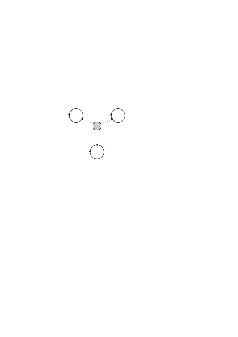
Figure 15: Triple-meson three-body interaction.

On the basis of the SU(3) properties of the ESC model, the changes of vector-meson masses in a nuclear medium induce the density-dependent effective repulsions in a rather universal manner in N​N, Y​N and Y​Y channels. Then, our first step is to investigate this effect in usual nuclear matter. Since for the scalar exchanges $\epsilon+P$ we expect big cancellations, also in the many-body case, we here for simplicity only change the vector-meson masses for an analysis of the sensitivity of e.g. the well-depths w.r.t. medium effects.

For convenience, our medium-induced effects are handled in comparison with the three-nucleon interaction (TNI) introduced by Lagaris-Pandharipande LaPa81 , which is represented in simple forms of density-dependent two-body interactions. Here, we refer their parameter sets TNI2 and TNI3, reproducing nuclear incompressibility 250 MeV and 300 MeV, respectively. Their TNI is composed of the attractive part (TNA) and the repulsive part (TNR). Our modeling for the repulsive component through the change of vector-meson masses corresponds only to their TNR. Hereafter, TNR (TNA) parts of TNI2 and TNI3 are denoted as TNR2 and TNR3 (TNA2 and TNA3), respectively.

Figure 16: Binding energy per nucleon $B/A$ in symmetric nuclear matter as a function of $\rho/\rho_{0}$ (saturation curve). The box represents the area in which saturation occurs empirically. In the left panel, the two solid curves show the G-matrix results for ESC04(N​N) with the QTQ and CIES prescriptions. In the right panel, the dashed curves are obtained by adding the TNI contributions on the QTQ result, and the solid curves are for the medium-corrected versions ESC04^∗(N​N). See the text for the detail.

In the left panel of Fig. 16, we show the saturation curves of symmetric nuclear matter, namely binding energy per nucleon as a function of $\rho$, which are obtained from the G-matrix calculations with ESC04(N​N). Here, the upper curve denoted as “QTQ” is calculated with the QTQ prescription. The lower one denoted as “CIES” is obtained with the choice of a continuous intermediate-energy spectrum in the G-matrix equation. The CIES result is known to simulate well the result including the three-hole line contributions Baldo . In the following procedure, however, we use the QTQ result because our G-matrix analyses for hypernuclear systems are based on the QTQ prescription in this paper. The box in the figure show the area where nuclear saturation is expected to occur empirically, and the energy minimums of both curves of “QTQ” and “CIES” are found to deviate from this area. In order to realize the nuclear saturation, three-body effects should be added on the contributions of ESC04(N​N) in the same way as the cases of using the other N​N interaction models: Here, we use the above mentioned TNI. The dashed curves in the right panel of Fig. 16 are obtained by adding the TNI contributions on the (QTQ) G-matrix results, where the reduction factor 0.8 is multiplied on the TNA part so as to give the energy minimum at an adequate value of $-15\ \sim\ -16$ MeV. The two curves in the figure correspond to the cases of adopting TNI2 and TNI3. Then, the saturation condition is found to be satisfied nicely. Hereafter, when we use the TNI together with ESC04(N​N), the factor 0.8 is always multiplied on the TNA part. In addition, the nucleon energy spectra obtained in the case of adopting TNI2 are adopted in the Y​N G-matrix equations in this work.

Next, we perform the G-matrix calculations with ESC04(N​N) in which the vector-meson masses are changed according to (47). Hereafter, the medium-corrected versions of ESC04 are denoted as ESC04${}^{*}(\alpha_{V})$ including the parameter $\alpha_{V}$. In the right side of Fig. 16, the two solid curves are obtained by adding the contributions of TNA2 and TNA3 multiplied by 0.8 to the G-matrix results. It should be noted here that the TNR parts are switched off because they are substituted by our medium-induced repulsions. Namely, the TNA parts are used here as phenomenological substitutes for the three-body attractive effects which are out of our present scope. The parameter $\alpha_{V}$ in (47) is chosen so as to simulate the TNR contributions: The two solid curves in the figure are obtained by choosing $\alpha_{V}=0.07$ fm³ and $\alpha_{V}=0.18$ fm³, which turn out to be quite similar to the dashed curves obtained by adding the TNI2 and TNI3 contributions, respectively, on the original G-matrix result. Thus, it turns out that the density dependence of our medium-induced repulsion is very similar to that of TNR. Although this similarity is of no fundamental meaning, it is nicely demonstrated that our medium-induced repulsion plays the same role as TNR for nuclear saturation.

Table 23: Calculated values of $U_{\Lambda}$ and $U_{\Sigma}$ at normal density for ESC04a-d${}^{*}(\alpha_{V}=0.18)$. Their $S$-state contributions are also given. All entries are in MeV.

		${}^{1/2,1}S_{0}$	${}^{1/2,3}S_{1}$		$U_{\Lambda}$		${}^{1/2,1}S_{0}$	${}^{1/2,3}S_{1}$	${}^{3/2,1}S_{0}$	${}^{3/2,3}S_{1}$		$U_{\Sigma}$
ESC04a∗		–12.0	–15.8		–30.6		12.2	–26.4	–11.0	8.6		–27.9
ESC04b∗		–11.6	–18.5		–33.0		10.1	–25.5	–9.0	15.2		–19.7
ESC04c∗		–12.3	–25.1		–39.3		7.9	–20.0	–10.3	12.7		–23.6
ESC04d∗		–12.0	–23.0		–37.2		8.3	–20.3	–9.6	19.1		–16.6

Let us study the effects of the medium corrections in the Y​N sectors of the ESC models. Then, a prospective way is to perform calculations for the values of $\alpha_{V}=0.07$ fm³ and $\alpha_{V}=0.18$ fm³ which induce repulsions similar to TNR2 and TNR3, respectively, in nucleon matter. In the following analysis, we investigate mainly the case of $\alpha_{V}=0.18$ fm³. In Table 23, the calculated values of $U_{\Lambda}$ and $U_{\Sigma}$ at normal density and their $S$-state contributions are shown in the case of taking $\alpha_{V}=0.18$ fm³. Comparing these values with those in Table 19 and Table 22, we find that the repulsive contributions are substantial both for $U_{\Lambda}$ and $U_{\Sigma}$. In the case of $U_{\Lambda}$, the $U_{\Lambda}$ values for ESC04a-d are too attractive in comparison with the empirical indication of $U_{\Lambda}\sim-30$ MeV. These overbinding values turn out to be improved substantially by our medium-induced repulsion. Especially, the values for ESC04a/b${}^{*}(\alpha_{V})$ are noted to agree well with the above empirical value. Similar repulsive contributions are seen also in the case of $U_{\Sigma}$, though the resulting values are still negative. However, it is important that the repulsive contribution is large in the ${}^{3}S_{1}(I=3/2)$ state, as discussed later.

It should be emphasized here that the spin-dependent features of the $\Lambda N$ G-matrix interaction are not really affected by our medium-induced repulsion. For instance, the values of $U_{\sigma\sigma}(S)$ become small only by 0.05 MeV (ESC04a), 0.09 MeV (ESC04b), 0.10 MeV (ESC04c) and 0.11 MeV (ESC04d) in the case of taking $\alpha_{V}=0.18$ fm³. In the cases of the $P$-state contributions such as $U_{\sigma\sigma}(P)$, $U_{LS}(P)$ and $U_{T}(P)$, the changes are negligibly small. The change of the effective mass $m^{*}_{\Lambda}$ is also small: The $m^{*}_{\Lambda}$ values for ESC04a-d${}^{*}(\alpha=0.18)$ are smaller by only $0.01\sim 0.02$ than those for ESC04a-d. These facts suggest interesting possibilities of using ESC04a-d${}^{*}(\alpha_{V})$ in various spectroscopic studies of $\Lambda$ hypernuclei, where the parameter $\alpha_{V}$ can be adjusted so as to reproduce experimental values of $B_{\Lambda}$ with almost no influence on spin-dependent structures of $\Lambda$ hypernuclei. Then, we stress that the meaning of the above choice $\alpha_{V}=0.18$ fm³ is only for its similarity to TNR3.

Figure 17: Calculated values of $U_{\Lambda}$ as a function of $\rho/\rho_{0}$. The three solid curves are for ESC04b, ESC04b${}^{*}(\alpha_{V}=0.07)$ and ESC04b${}^{*}(\alpha_{V}=0.18)$. The two dashed curves are obtained by adding the TNR2 and TNR3 contributions on the result for ESC04b. See the text for the detail.

Our medium-induced repulsions are related intimately to the problem of maximum masses of neutron stars. As well known, the repulsive three-body force in high-density neutron matter, embodied in TNR, plays an essential role for a stiffening of the EOS of neutron-star matter, assuring the observed maximum mass of neutron stars. However, the hyperon mixing in neutron-star matter brings about the remarkable softening of the EOS, which cancels the effect of the repulsive three-body force for the maximum mass. In order to avoid this serious problem, Nishizaki, Takatsuka and one of the authors (Y.Y.) TNY02 ; NYT01 introduced the conjecture that the TNR-type repulsions work universally for ${\it YN}$ and ${\it YY}$ as well as for $N\!N$. They showed that the role of the TNR for stiffening the EOS can be recovered clearly by this assumption. Our model of the medium-induced repulsion explains their assumption quite naturally. In Fig. 17, we draw the values of $U_{\Lambda}$ as a function of $\rho/\rho_{0}$ in some cases: The three solid curve are for ESC04b and ESC04b${}^{*}(\alpha_{V}=0.07)$ and ESC04b${}^{*}(\alpha_{V}=0.18)$, and the two dashed curves are obtained by adding the TNR2 and TNR3 contributions on the result for ESC04b. It is found, here, our medium-induced repulsions for $\alpha_{V}=0.07$ and $\alpha_{V}=0.18$ are very similar to the TNR2 and TNR3 contributions, respectively, as well as the case of nuclear saturation curves. Thus, it is clearly demonstrated that our medium-induced repulsions, which works universally among octet baryons, will assure the stiffening of the EOS.

In neutron-star matter, the chemical equilibrium condition for $\Sigma^{-}$ given by $\mu_{\Sigma^{-}}=\mu_{n}+\mu_{e^{-}}$ makes $\Sigma^{-}$ mixing more favorable than $\Lambda$ mixing controlled by $\mu_{\Lambda}=\mu_{n}$ in cases of neglecting strong interactions. Then, it is an important problem whether the well depth of $\Sigma^{-}$ is attractive or repulsive in neutron matter. As shown in Table 23, our medium-induced repulsion for $\Sigma N$ contributes dominantly in the ${}^{3}S_{1}(I=3/2)$-state with the largest statistical weight. Thus, this repulsive effect appears most strongly in the $\Sigma^{-}$ well depth in neutron matter given by the $I=3/2$ $\Sigma N$ interaction.

In our analysis for hypernuclear systems, we do not consider the three-body attraction, such as TNA, which plays an important role for nuclear saturation as well as the three-body repulsion such as TNR and our medium-induced effect. The origin of such a part is considered to be in meson-exchange three-body correlations, being initiated by Fujita-Miyazawa FM . Possible counterparts in our hyperonic matter will be studied in future.

X.3 Double-$\Lambda$ states

Here, we study the $\Lambda\Lambda$ $(^{11}S_{0})$ interactions, for which the experimental information can be obtained from the data of double-$\Lambda$ hypernuclei. In the past, NHC-D NRS77 has been used popularly as a standard meson-theoretical model for $S=-2$ interactions. The reason was because this interaction is compatible with strong $\Lambda\Lambda$ attraction ($\Delta B_{\Lambda\Lambda}=4\sim 5$ MeV) supported by earlier data on double-$\Lambda$ hypernuclei. This strong $\Lambda\Lambda$ attraction of NHC-D is due to its specific feature that only the scalar singlet meson is taken into account. Since the discovery of NAGARA event identified uniquely as ${}^{\ 6}_{\Lambda\!\Lambda}$He Tak01 in 2001, the $\Lambda\Lambda$ interaction is established to be rather less attractive ($\Delta B_{\Lambda\!\Lambda}\approx 1$ MeV). Then, it is quite important to investigate what values of $\Delta B_{\Lambda\!\Lambda}$ are obtained for ESC04 models.

Let us here evaluate the values of $\Delta B_{\Lambda\!\Lambda}(^{\ 6}_{\Lambda\!\Lambda}$He), taking account of the $\Lambda\Lambda$-$\Xi N$ coupling effect explicitly. For this purpose, we adopt the three-body model composed of the $\alpha\!+\!\Lambda\!+\!\Lambda$ and $\alpha\!+\!\Xi\!+\!N$ configurations. The effective $\Lambda\Lambda$-$\Lambda\Lambda$ and $\Lambda\Lambda$-$\Xi N$ interactions Lans04 are derived in the G-matrix framework as follows: We solve the $\Lambda\Lambda$-$\Xi N$-$\Sigma\Sigma$ coupled-channel G-matrix equation for a $\Lambda\Lambda$ pair in nuclear matter, and represent the resultant $\Lambda\Lambda$-$\Lambda\Lambda$ and $\Lambda\Lambda$-$\Xi N$ G-matrices as local potentials in coordinate space. These G-matrix interactions depend on the nucleon Fermi momentum $k_{F}$ of nuclear matter. Then, it is a problem what value of $k_{F}$ should be chosen in our calculation for ${}^{\ 6}_{\Lambda\!\Lambda}$He. In similar calculations for ${}^{5}_{\Lambda}$He, the value of $k_{F}$ parameter included in the $\Lambda N$ G-matrix interaction was chosen around 1.0 fm^-1 Yam85 . This value of $k_{F}\sim 1.0$ fm^-1 agree qualitatively with the value derived from the average nuclear density felt by the $\Lambda$ particle in ${}^{5}_{\Lambda}$He. Because a sophisticated estimation of the $k_{F}$ value is not necessary for our purpose of demonstrating features of the interaction models, we choose this plausible value of $k_{F}$= 1.0 fm^-1 in the present calculations for ${}^{\ 6}_{\Lambda\!\Lambda}$He.

Using our $\Lambda\Lambda$-$\Lambda\Lambda$ and $\Lambda\Lambda$-$\Xi N$ G-matrix interactions, three-body variational calculations are performed in the Gaussian basis functions Yama89 , where the $\Xi N$-$\Xi N$ interaction is not taken into account for simplicity. It should be noted that in our approach high-lying $\Lambda\Lambda$-$\Xi N$-$\Sigma\Sigma$ correlations are renormalized into the $\Lambda\Lambda$-$\Lambda\Lambda$ and $\Lambda\Lambda$-$\Xi N$ G-matrices, and low-lying $\Lambda\Lambda$-$\Xi N$ correlations are treated in the model space composed of $\alpha\!+\!\Lambda\!+\!\Lambda$ and $\alpha\!+\!\Xi\!+\!N$ configurations. In order to avoid the double counting of the $\Lambda\Lambda$-$\Xi N$ coupling interaction, it is necessary that the high-lying $\Lambda\Lambda$-$\Xi N$ correlations are not included in our three-body model space. A practical way for this problem is to take the two $\Lambda$ ($\Xi$ and $N$) coordinates from the center of mass of $\alpha$ core, not the relative coordinate between them explicitly, because the short-range correlations are taken into account unfavorably in this model space.

As for the interactions between the $\alpha$ cluster and valence particles ($\Lambda$, $\Xi$, $N$), we adopt the phenomenological potentials: For $\alpha$-$\Lambda$ and $\alpha$-$\Xi$ interactions, we use the two-range Gaussian potentials given in Ref.Lans04 . Here, the former is fitted so as to reproduce the $\Lambda$ binding energies of ${}^{4}_{\Lambda}$H and ${}^{4}_{\Lambda}$He. The strength of the latter (named as Xa1 Lans04 ) is determined in consideration of the experimental indication that the $\Xi$ well depth is roughly half of the $\Lambda$ one. On the other hand, we use the Kanada-Kaneko potential Kanada for the $\alpha$-$N$ interaction, designed so as to reproduce scattering phase shifts. In the $\alpha\!+\!\Xi\!+\!N$ channel, we take into account the orthogonality condition between $\alpha$ and $N$.

Table 24: $\Delta B_{\Lambda\!\Lambda}(^{\ 6}_{\Lambda\!\Lambda}$He) values (in MeV) are calculated with G-matrix interactions derived from ESC04a-d, NSC97 and NHC-D. (The hard-core radius in NHC-D is taken as 0.53 fm.)

		$\Delta B_{\Lambda\!\Lambda}$ (MeV)	$P_{\Xi N}$ (%)
ESC04a		1.36	0.44
ESC04b		1.37	0.45
ESC04c		0.97	1.15
ESC04d		0.98	1.18
NSC97f		0.34	0.19
NHC-D		1.05	0.14

In Table 24 we show the calculated values of $\Delta B_{\Lambda\!\Lambda}(^{\ 6}_{\Lambda\!\Lambda}$He) and $\Xi N$ admixture probabilities $P_{\Xi N}$ in the cases of using ESC04a-d, NSC97f and NHC-D. (In the calculation for NHC-D, the hard-core radius in the ${}^{11}S_{0}$ state is taken as 0.53 fm, and the $\Sigma\Sigma$ channel is not taken into account.) The effect of the medium-induced repulsion is not so remarkable in this case, because the $\Lambda\Lambda$ G-matrix is calculated at low density ($k_{F}=$ 1.0 fm^-1). For instance, the calculated values for ESC04a${}^{*}(\alpha=0.18)$ are $\Delta B_{\Lambda\!\Lambda}$=1.24 MeV and $P_{\Xi N}$=0.44 %. The calculated $\Delta B_{\Lambda\!\Lambda}$ values should be compared with the experimental value $1.01\pm 0.20^{+0.18}_{-0.11}$ MeV Tak01 . Then, the calculated values for ESC04a-d are considered to be more or less reasonable in the present scope of our simple three-body model.

On the other hand, the value of $\Delta B_{\Lambda\!\Lambda}$ for NSC97f turns out to be rather too small compared with the experimental value: The $\Lambda\Lambda$ interaction of NSC97f is concluded to be too weak. It is interesting that our result for NSC97f is quite similar to the Yamada’s result Yamada04 , obtained from the sophisticated variational calculation with direct use of NSC97f. This means that our model-space approach with G-matrix effective interactions simulates nicely the real space approach with free-space interactions. It was pointed out by Yamada that the $\Lambda\Lambda$-$\Xi N$-$\Sigma\Sigma$ coupling treatment leads to the less $\Lambda\Lambda$ binding than the $\Lambda\Lambda$-$\Xi N$ one due to the existence of a pseudo bound state in the case of NSC97f. It should be noted that such a pseudo bound state does not appear in the case of ESC04a-d. In Vidana the similar result was obtained for NSC97f by the G-matrix calculation. On the other hand, the importance of the rearrangement effect of the $\alpha$-core for $\Delta B_{\Lambda\Lambda}(^{6}_{\Lambda\Lambda}$He) has been pointed out by Kohno03 ; Usmani04 ; Nemu05 . It is an open problem to study core-rearrangement effects on the basis of the ESC04 models.

The most striking feature of ESC04a-d is the far stronger $\Lambda\Lambda$-$\Xi N$ coupling than NSC97f and NHC-D. In Table 24, this feature is seen in larger value of $P_{\Xi N}$ in the case of ESC04a-d. In particular, it is very curious that the $\Lambda\Lambda$-$\Xi N$ couplings of ESC04c/d are extremely strong. As shown in Ref. Lans04 , such a coupling effect appears dramatically in ${}^{\ 5}_{\Lambda\!\Lambda}$H and ${}^{\ 5}_{\Lambda\!\Lambda}$He because of the small energy differences between ground $\Lambda$-$\Lambda$ states and $\Xi$-$\alpha$ states. A comprehensive study on the $\Lambda\Lambda$-$\Xi N$ coupling is now in progress on the basis of ESC04a-d.

X.4 Properties of $\Xi N$ G-matrix

There is no $\Xi N$ scattering data at present. We have only uncertain information on $\Xi$-nucleus interactions experimentally. We consider that the most reliable data in the present stage was given by the BNL-E885 experiment E885 , in which they measured the missing mass spectra for the ¹²C$(K^{-},K^{+})$X reaction. Reasonable agreement between this data and theory is realized by assuming a $\Xi$-nucleus potential $U_{\Xi}(\rho)=-V_{0}f(r)$ with well depth $V_{0}\sim 14$ MeV within the Wood-Saxon (WS) prescription.

Let us here derive the potential energies $U_{\Xi}$ using the G-matrix theory in the same way as the cases of $U_{\Lambda}$ and $U_{\Sigma}$. In the past, NHC-D gave rise to attractive values of $U_{\Xi}$, while strongly repulsive values were obtained for the other Nijmegen models. Then, it is very curious what values of $U_{\Xi}$ are obtained for ESC04a-d.

In the same way as in the $\Sigma N$ case, we solve the $\Xi N$ starting channel G-matrix equation in the QTQ prescription. Likewise, the $\Xi$ conversion width $\Gamma_{\Xi}$, due to an energy-conserving $\Xi N$-$\Lambda\Lambda$ transition, is not calculated here. In this case, the channel-coupling treatments are performed for $\Lambda\Lambda$-$\Xi N$-$\Sigma\Sigma$ and $\Xi N$-$\Lambda\Sigma$-$\Sigma\Sigma$ channels.

Table 25: Values of $U_{\Xi}$ at normal density and partial wave contributions for ESC04a-d and ESC04d${}^{*}(\alpha_{V}=0.18)$. For comparison, the result for NHC-D is also shown (hard-core radii are taken as 0.50 fm in all channels.). All entries are in MeV.

	$T$		${}^{1}S_{0}$	${}^{3}S_{1}$	${}^{1}P_{1}$	${}^{3}P_{0}$	${}^{3}P_{1}$	${}^{3}P_{2}$		$U_{\Xi}$
ESC04a	0		8.1	–10.0	1.0	–0.3	–0.4	–0.7
	1		–4.5	21.8	–0.7	0.7	–0.1	0.3		+15.1
ESC04b	0		5.9	–2.4	0.7	0.7	1.0	–0.4
	1		0.5	27.9	0.6	0.9	–0.3	1.2		+36.3
ESC04c	0		5.9	–15.7	1.2	–0.1	–1.8	–1.2
	1		6.8	1.9	–0.8	0.1	–0.3	–1.7		–5.5
ESC04d	0		6.4	–19.6	1.1	1.2	–1.3	–2.0
	1		6.4	–5.0	–1.0	–0.6	–1.4	–2.8		–18.7
ESC04d∗	0		6.3	–18.4	1.2	1.5	–1.3	–1.9
	1		7.2	–1.7	–0.8	–0.5	–1.2	–2.5		–12.1
NHC-D	0		–4.5	2.6	–1.8	–0.2	–0.6	–1.7
	1		0.2	5.3	–2.6	0.0	–2.9	–5.6		–11.9

In Table 25 we show the calculated values of $U_{\Xi}$ at normal density and their partial-wave contributions for ESC04a-d and ESC04d${}^{*}(\alpha_{V}=0.18)$. For comparison, the result for NHC-D is also given, where the hard-core radii are taken as 0.50 fm in all channels, and the $\Sigma\Sigma$ and $\Lambda\Sigma$ channels are not taken into account. Now, the remarkable difference among ESC04a-d is revealed: These four versions turn out to give rise to completely different values of $U_{\Xi}$. It should be noted that the ESC models such as ESC04c/d can bring about attractive $\Xi$-nucleus potentials predicting the existence of $\Xi$ hypernuclei. It is very interesting that ESC04d^∗ including the medium-induced repulsion leads to the $\Xi$ well depth similar to the above “experimental” value. Though the attractive value of $U_{\Xi}$ is obtained also in the case of NHC-D, its partial-wave contribution is completely different from those in the case of ESC04c/d. In the former case, the attractive $U_{\Xi}$ is owing to the strong $P$-state attraction. In the latter case, however, the strong attraction in the ${}^{13}S_{1}$ state plays an essential role for it. Because of this reason, various $\Xi$ hypernuclear states will be predicted even in light $s$-shell systems on the basis of ESC04c/d. Level structures of these $\Xi$ states have to reflect the peculiar spin- and isospin dependences of the underlying $\Xi N$ interactions. The detailed analysis will be given in our next paper.

XI Discussion and Conclusions

We have shown in this paper that the ESC-approach to the nuclear force problem is able to make a connection between on the one hand the at present available baryon-baryon data and on the other hand the underlying quark structure of the baryons and mesons. Namely, a successfull description of both the N​N- and Y​N-scattering data is obtained with meson-baryon coupling parameters which are almost all explained by the QPC-model. This at the same time in obediance of the strong constraint of no bound states in the $S=-1$-systems. Therefore, the ESC04 models of this paper are an important step in the determination of the baryon-baryon interactions for low energy scattering and the description of hypernuclei in the context of broken SU(3)-symmetry. The values for many parameters, which in previous work were considered to free to large extend, are now limited strongly, and tried to be made consistent with the present theoretical view on low energy hadron physics. This is in particularly the case for the $F/(F+D)$-ratios of the MPE-interactions. These ratio’s for the vector- and scalar-mesons are rather close to the QPC-model predictions. This holds also for the values of the coupling constants. Here, the introduction of a zero in the form factor is important, leading to a sizeable reduction in the scalar couplings. It is interesting that the features of $\sigma$-exchange with a zero in the form factor are very similar to those obtained in a chiral-unitary-approach Ose00 .

The application of the $Q\bar{Q}$-pair creation to baryon-meson couplings using a ${}^{3}S_{1}$-model Zha84 for pseudoscalar and vector-meson couplings, and the nucleon-nucleon interactions has first been attempted by Fujiwara and Hecht Fuj92 . We did not explore this possibility, but it is not unlikely that this alternative leads to a similar scheme of couplings as the ${}^{3}P_{0}$-model.

The G-matrix results show that basic features of hypernuclear data are reproduced nicely by ESC04, improving some weak points of the soft-core OBE-models NSC89 MRS89 and NSC97 RSY99 . In spite of this superiority of ESC04 for hypernuclear data, perhaps not every aspect of the effective (two-body) interactions in hypernuclei can be described by this model. For example, this could be the case for the well depth $U_{\Sigma}$. From the results it is clear that a good fit to the scattering data not necessarily means success in the G-matrix results. To explain this one can think of two reasons: (i) the G-matrix results are sensitive to the two-body interactions below 1 fm, whereas the present YN-scattering data are not, (ii) other than two-body forces play an important role. However, since the ${\it NN}\oplus{\it YN}$-fit is so much superior for ESC04- than for OBE-models, we are inclined to look for solutions to the mentioned problems outside the two-body forces. A natural possibility is the presence of three-body forces (3BF) in hypernuclei which can be viewed as generating effective two-body forces, which could solve the well-depth issues. In the case of the $\Delta B_{\Lambda\Lambda}$ also 3BF could be operating. This calls for an evaluation of the 3BF’s $NNN$, $\Lambda NN$, $\Sigma NN$, $\Lambda\Lambda N$, etc. for the soft-core ESC-model, consistent with its two-body forces.

The $\Lambda N$ p-waves seem to be better, which is the result of the truly simultaneous $NN+{\it YN}$-fitting. This is also reflected in the better $K_{\Lambda}$-value, making the well-known small spin-orbit splitting smaller.

Finally, we mention the extensive work on baryon-baryon using the resonating-group-method (RGM), exploiting quark-gluon-exchange (QGE) in conjunction with OBE, taking full account of the antisymmetrization of the six quarks in the two-baryon systems Fuj02 . A remarkable difference with the ESC-models is that QGE leads to strong repulsion in the $\Sigma N(^{3}S_{1},I=3/2)$- and the $\Sigma N(^{1}S_{0},I=1/2)$-channels. In contrast, in this paper we have assumed that QGE is very suppressed dynamically.

- (1) Th.A. Rijken, Extended-soft-core Baryon-Baryon Model, I. Nucleon-Nucleon Scattering , submitted to Phys. Rev. C.
- (2) Th.A. Rijken and Y. Yamamoto, Extended-soft-core Baryon-Baryon Model, III. etc. Scattering , in preparation.
- (3) P.M.M. Maessen, Th.A. Rijken, and J.J. de Swart, Phys. Rev. C 40 (1989) 2226.
- (4) Th.A. Rijken, V.G.J. Stoks, and Y. Yamamoto, Phys. Rev. C 59, 21, (1999).
- (5) T.A. Rijken, Ann. Phys. (N.Y.), 164 (1985) 1,23.
- (6) T.A. Rijken, in Few-Body Problems in Physics ‘99, Proceedings of the 1st Asian-Pacific Conference, August 23-28, Tokyo, p. 317, Editors S. Oryu, M. Kamimura, and S. Ishikawa, Springer-Verlag (2000).
- (7) T.A. Rijken, Nucl. Phys. A 691 (2001) 322c-328c.
- (8) L. Micu, Nucl. Phys. B10 (1969) 521; R. Carlitz and M. Kislinger, Phys. Rev. D 2 (1970) 336.
- (9) Y. Yamamoto and H. Bandō, Progr. Theor. Phys. 83 (1990) 254.
- (10) T. Motoba and Y. Yamamoto, Nucl. Phys. A 585 (1995) 29c.
- (11) T. Hasegawa et al., Phys. Rev. Lett. 74 (1995) 224.
- (12) R.H. Dalitz and F. von Hippel, Phys. Lett. 10, 153 (1964).
- (13) M.M. Nagels, T.A. Rijken, and J.J. de Swart, Ann. Phys. (N.Y.) 79, 338 (1973).
- (14) J.J. de Swart, Rev. Mod. Phys. 35 (1963) 916; ibid. 37 (1965) 326(E).
- (15) P.A. Carruthers, ’Introduction to unitary symmetry’, John Wiley & Sons Inc., New York , 1966.
- (16) R.E. Marshak, Riazuddin, and C.P. Ryan, ’Theory of weak interactions in particle physics’, John Wiley & Sons Inc., New York , 1969.
- (17) A. Le Yaouanc, L. Oliver, O. Péne, and J.-C. Raynal, Phys. Rev. D 8 (1973) 2223; Phys. Rev. D 11 (1975) 1272.
- (18) M. Chaichain and R. Kögerler, Ann. Phys. (N.Y.) 124 (1980) 61.
- (19) M.M. Nagels, T.A. Rijken, and J.J. de Swart, Phys. Rev. D 17 (1978) 768.
- (20) R.A. Bryan and A. Gersten, Phys. Rev. D 6 (1972) 341.
- (21) V.G.J. Stoks, R.A.M. Klomp, M.C.M. Rentmeester, and J.J. de Swart, Phys. Rev. C 48 (1993) 792.
- (22) R.A.M. Klomp, private communication (unpublished).
- (23) J.K. Ahn et al, Nucl. Phys. A761 (2005) 41. H. Kanda, Tohoku University Sendai, KEK-experiment E289, private communication 2005; J.K. Ahn et al, Nucl. Phys. A761 (2005) 41.
- (24) Th.A. Rijken and V.G.J. Stoks, Phys. Rev. C 54 (1996) 2869; ibid. C 54 (1996) 2869.
- (25) V.G.J. Stoks and Th.A. Rijken, Nucl. Phys. A 613 (1997) 311.
- (26) G. Alexander, U. Karshon, A. Shapira, G. Yekutieli, R. Engelmann, H. Filthuth, and W. Lughofer, Phys. Rev. 173, 1452 (1968).
- (27) B. Sechi-Zorn, B. Kehoe, J. Twitty, and R.A. Burnstein, Phys. Rev. 175, 1735 (1968).
- (28) F. Eisele, H. Filthuth, W. Fölisch, V. Hepp, E. Leitner, and G. Zech, Phys. Lett. 37B, 204 (1971).
- (29) R. Engelmann, H. Filthuth, V. Hepp, and E. Kluge, Phys. Lett. 21, 587 (1966).
- (30) V. Hepp and M. Schleich, Z. Phys. 214, 71 (1968).
- (31) D. Stephen, Ph.D. thesis, University of Massachusetts, 1970. Z. Phys. 214, 71 (1968).
- (32) J.J. de Swart and C. Dullemond, Ann. of Phys. 19 (1962) 458.
- (33) J.J. de Swart, M.M. Nagels, T.A. Rijken, and P.A. Verhoeven, Springer Tracts in Modern Physics, 60 (1971) 138.
- (34) Y. Fujiwara, T. Fujita, C. Nakamoto, and Y. Suzuki, Progr. Theor. Phys. 100 (1998) 957.
- (35) ESC04 YN-potentials, see http://nn-online.org.
- (36) B. Sakita and K.C. Wali, Phys. Rev. 139 (1965) B1355.
- (37) E. Hiyama, M. Kamimura, T. Motoba, T. Yamada and Y. Yamamoto, Phys. Rev. C 65 (2001) 011301(R).
- (38) A. Nogga, H. Kamada, and W. Glöckle, Phys. Rev. Lett. 88 (2002) 172501.
- (39) H. Nemura, Y. Akaishi, and Y. Suzuki, Phys. Rev. Lett. 89 (2002) 142504.
- (40) D.J. Millener, Nucl. Phys. A691 (2001) 93c.
- (41) R.R. Scheerbaum, Nucl. Phys. A257 (1976) 77.
- (42) E. Hiyama, M. Kamimura, T. Motoba, T. Yamada, and Y. Yamamoto, Phys. Rev. Lett. 85 (2000) 270.
- (43) Y. Fujiwara, M. Kohno, K. Miyagawa, and Y. Suzuki, Phys. Rev. C70 (2004) 047002.
- (44) Y. Yamamoto, S. Nishizaki, and T. Takatsuka, Prog. Theor. Phys. 103 (2000) 981.
- (45) C.J. Batty, E. Friedman, and A. Gal, Prog. Theor. Phys. Suppl. No.117 (1994) 227.
- (46) J. Dabrowski, Phys. Rev. C 60 (1999) 025205.
- (47) H. Noumi et al., Phys. Rev. Lett. 89 (2002) 072301.
- (48) M. Kohno, Y. Fujiwara, Y. Watanabe, K. Ogata, and M. Kawai, Prog. Theor. Phys. 112 (2004) 895.
- (49) A.D. Jackson, Ann. Rev. Nucl. Part. Sci. 33 105 (1983); A.D. Jackson, E. Krotcheck, and M. Rho, Nucl. Phys. A407 (1983) 495.
- (50) I.E. Lagaris and V.R. Pandharipande, Nucl. Phys. A359 (1981) 349.
- (51) M. Baldo, A. Fiasconaro, H.Q. Song, G. Giansiracusa, and U. Lombardo, Phys. Rev. C 65 (2002) 017303.
- (52) T. Takatsuka, S. Nishizaki, and Y. Yamamoto, Proc. Int. Symp. on Perspectives in Physics with Radiactive Isotopes, Hayama, Kanagawa, Japan, Nov. 13-16, 2000 ; Eur. Phys. J. A. 13 (2002) 213.
- (53) S. Nishizaki, and Y. Yamamoto, T. Takatsuka, Prog. Theor. Phys. 105 (2001) 607; ibid 108 (2002) 703.
- (54) J. Fujita and H. Miyazawa, Prog. Theor. Phys. 17 (1957) 360; 17 (1957) 366.
- (55) M.M. Nagels, T.A. Rijken, and J.J. deSwart, Phys. Rev. D 15 (1977) 2547.
- (56) H. Takahashi et al., Phys. Rev. Lett. 87 (2001) 212502.
- (57) D.E. Lanskoy and Y. Yamamoto, Phys. Rev. C 69 (2004) 014303.
- (58) Y. Yamamoto and H. Bandō, Prog. Theor. Phys. Suppl. No.81 (1985) 9.
- (59) Y. Yamamoto, H. Takaki, and K. Ikeda, Prog. Theor. Phys. 82 (1989) 13.
- (60) H. Kanada, T. Kaneko, S. Nagata, and M. Nomoto, Prog. Theor. Phys. 61 (1979) 1327.
- (61) T. Yamada, Phys. Rev. C69 (2004) 044301.
- (62) I. Vidaña, A. Ramos, and A. Polls, Phys. Rev. C70 (2004) 024306.
- (63) M. Kohno, Y. Fujiwara, and Y. Akaishi, Phys. Rev. C68 (2003) 034302.
- (64) Q.N. Usmani, A.R. Bodmer, and Bhupali Sharma, Phys. Rev. C70 (2004) 061001(R).
- (65) H. Nemura, S. Shinmura, Y. Akaishi, and Khin Swe Myint, Phys. Rev. Lett. 94 (2005) 202502.
- (66) P. Khaustov et al., Phys. Rev. C 61 (2000) 054603.
- (67) E. Oset, H. Toki, M. Mizobe, and T.T. Takahashi, Progr. Theor. Phys. 103 (2000) 351.
- (68) Y.W. Yu and Z.Y. Zhang, Nucl. Phys., A426 (1984) 557.
- (69) Y. Fujiwara, Progr. Theor. Phys. 88 (1992) 933, and the references cited here.
- (70) Y. Fujiwara, T. Fujita, M. Kohno, C. Nakamoto, and Y. Suzuki, Phys. Rev. C 65 (2002) 014002, and cited references.