Extended-soft-core Baryon-Baryon Model
I. Nucleon-Nucleon Scattering (ESC04)

Abstract

The NN results are presented from the extended-soft-core (ESC) interactions. They consist of local- and non-local-potentials due to (i) one-boson-exchanges (OBE), which are the members of nonets of pseudoscalar-, vector-, scalar-, and axial-mesons, (ii) diffractive-exchanges, (iii) two-pseudoscalar-exchange (PS-PS), and (iv) meson-pair-exchange (MPE). We describe a fit to the pp- and np-data for $0\leq T_{\rm lab}\leq 350$ MeV, having a typical $\chi^{2}/N_{\rm data}=1.155$. Here, we used ca 20 quasi-free physical parameters, being coupling constants and cut-off masses. A remarkable feature of the couplings is that we were able to require them to follow rather closely the pattern predicted by the ${}^{3}P_{0}$ quark-pair-creation (QPC) model. As a result the 11 OBE-couplings are rather constrained, i.e. quasi-free. Also, the deuteron binding energy and the several NN scattering lengths are fitted.

I Introduction

In a series of three papers we present the results recently obtained with the extended-soft-core (ESC) model Rij93 for nucleon-nucleon (NN), hyperon-nucleon (YN), and hyperon-hyperon (YY) with $S=-2$. For NN Rij93 ; RS96a ; RS96b ; SR97 ; RPN02 it has been demonstrated that the ESC-model interactions give an excellent description of the NN-data. Also for YN the first attempts Rij99 ; Rij00 showed that the ESC-approach is potentially rather promising to give improvements w.r.t. the one-boson-exchange (OBE) soft-core models MRS89 ; RSY99 . As compared to the earlier versions of the ESC-model, we introduce in these papers two innovations. First, we introduce a zero in the form factor of the scalar mesons. Secondly, we exploit the exchange of the axial-vector mesons. In this first paper of the series, we display the recent results fitting exclusively the NN-data, giving the NN-model presented in this paper ESC04(NN). In the second paper, henceforth referred to as II RY04b , we report on the results for ${\it NN}\oplus{\it YN}$, in a simultaneous fit of the NN- and YN-data. This is a novelty w.r.t. our procedure described in previous publications on the Nijmegen work. The advantages will be discussed in II. In the third paper, henceforth referred to as III RY04c , we will report on the predictions for YN and YY with $S=-2$.

A general modern theoretical framework for the soft-core interactions is provided by the so called standard-model (SM). Starting from the SM we consider the stage where the heavy quarks are integrated out, leaving an effective QCD-world for the u,d,s quarks. The generally accepted scenario is now that the QCD-vacuum is unstable for momentum transfers for which $Q^{2}\leq\Lambda_{\chi SB}^{2}\approx 1$ GeV² Geo93 , causing spontaneous chiral-symmetry breaking ($\chi$SB). A phase-transition of the vacuum generates constituent quark masses via $\langle 0|\bar{\psi}\psi|0\rangle\neq 0$, and thereby the gluon coupling $\alpha_{s}$ is reduced substantially. In view of the small pion mass, the Nambu-Goldstone bosons associated with the spontaneous $\chi SB$ are naturally identified with the pseudoscalar mesons. Also, as a result of the phase-transition the dominating degrees of freedom are the baryons and mesons. In this context, low-energy baryon-baryon interactions are described naturally by meson-exchange using form factors at the meson-baryon vertices. This way, the phase transition has transformed the effective QCD-world into an effective hadronic-world. To reduce this complex world with its numerous degrees of freedom, we consider a next step. This is, envisioning the integrating out of the heavy mesons and baryons using a renormalization procedure a la Wilson Pol84 , we restrict ourselves to mesons with $M\leq 1$ GeV$/c^{2}$, arriving at a so-called effective field theory as the proper arena to describe low energy baryon-baryon scattering. This is the general physical basis for the Nijmegen soft-core models.

Because of the composite nature of the mesons in QCD, the proper description of meson-exchange is quite naturally in terms of Regge-trajectories. For example, in the Bethe-Salpeter approach to the $Q\bar{Q}$-system any reasonable interaction leads to Regge poles. Therefore, in the Nijmegen soft-core approach meson-exchange is treated as the dominant part of the mesonic reggeon-exchange. This includes also the $J=0$ contributions from the tensor trajectories ($f_{2}$,$f_{2}^{\prime}$ and $A_{2}$). In elastic scattering we notice that the most important exchange at higher energies is pomeron-exchange. Therefore in the soft-core OBE-models NRS78 the traditional OBE-model was extended by including the pomeron, and the pomeron parameters determined from the low-energy NN-data were in good agreement with those found at high energy. This feature is also found to persist in the ESC-models. For a more elaborate discussion of the pomeron, and its importance for the implementation of chiral-symmetry in the soft-core models, we refer to MRS89 ; Pad89 .

The dynamics in the ESC-model is constructed employing the following mesons together with flavor SU(3)-symmetry:

1. The pseudoscalar-meson nonet $\pi,\ \eta,\ \eta^{\prime},\ K$ with the $\eta-\eta^{\prime}$ mixing angle $\theta_{P}=-23.0^{0}$ from the Gell-Mann-Okubo mass formula.

2. The vector-meson nonet $\rho,\ \phi,\ K^{\star},\ \omega$ with the $\phi-\omega$ ideal mixing angle $\theta_{V}=37.56^{0}$.

3. The axial-vector-meson nonet $a_{1},f_{1}\ K_{1},f_{1}^{\prime}$ with the $f_{1}-f_{1}^{\prime}$ mixing angle $\theta_{A}=47.3^{0}$ SR97 .

4. The scalar-meson nonet $a_{0}(962)=\delta,\ f_{0}(993)=S^{\star},\ \kappa,f_{0}(760)=\varepsilon$ with a free $S^{\star}-\varepsilon$ mixing angle $\theta_{S}$ to be determined in a fit to the YN-data.

5. The ‘diffractive’ contribution from the pomeron P, and the tensor-mesons $f_{2}$, $f_{2}^{\prime}$, and $A_{2}$. These interactions will give mainly repulsive contributions of a gaussian type to the potentials in all channels. In the present ESC-model we have taken $g_{A_{2}}=g_{BBf_{2}}=g_{BBf_{2}^{\prime}}=0$, i.e. only the pomeron contributes.

The BBM-vertices are described by: (i) coupling constants and $F/(F+D)$-ratio’s obeying broken flavor SU(3)-symmetry, see paper II for details, and (ii) gaussian form factors. This type of form factor is like the often used residue functions in Regge phenomenology. Also, from the point of view of the (nonrelativistic) quark models a gaussian behavior of the form factors is most natural. Here, we remark that in the ESC-models the two-meson-cut contributions to the form factors are taken into account using meson-pair exchanges (MPE) (see below). Evidently, with cut-off masses $\Lambda\approx 1$ GeV, these form factors assure a soft behavior of the potentials in configuration space at small distances. The form factors depend on the SU(3) assignment of the mesons, as described in detail in RSY99 .

The potentials of the ESC-model are generated by

1. One-boson-exchange (OBE). The treatment of the OBE in the soft-core approach has been given for NN in NRS78 , and for YN in MRS89 . With respect to these OBE-interactions the present ESC-model contains, as mentioned above, two innovations. First, in the scalar meson form-factor we have introduced a zero. This zero is natural in the ${}^{3}P_{0}$-pair-creation (QPC) Mic69 ; Yao73 ; Yao75 model for the coupling of the mesonic quark-antiquark ($Q\bar{Q}$) system to baryons. The scalar meson, being itself in this picture a ${}^{3}P_{0}$ $Q\bar{Q}$-bound state, gets a zero when it couples to a baryon. A pragmatic reason to exploit such a zero is that in this way we were able to avoid a bound state in $\Lambda N$-scattering. Secondly, for the first time we incorporated axial-meson exchange in the potentials. As is well known, they are considered as the chiral partners of the vector mesons. It turned out that the strength of the axial-meson exchanges is found to agree with the theoretical determination $g_{a_{1}}\approx(m_{a_{1}}/m_{\pi})f_{NN\pi}$ Sch68 .

2. Two-meson-exchange (TME). The configuration space soft-core uncorrelated two-meson exchange for NN has been derived in Rij91 ; RS96a . We use these potentials in this paper for PS-PS exchange. Here, we give a complete SU(3)-symmetry treatment in NN, as well as in YN and YY. For example, we include double $K$-exchange in NN-scattering. Similarly in papers II and III their generalization to YN respectively YY. The PS-PS potentials contain the important long-range two-pion potentials. The other kind of two-meson exchange, as pseudoscalar-vector (PS-V), and pseudoscalar-scalar (PS-S) etc. are supposed to be less important, because of cancellations, and can be covered by OBE in an effective manner. Of course, this gives some contamination in the meson-baryon coupling constants.

3. Meson-pair-exchange (MPE). These have been described for NN and justified in RS96b . Again, in II and III the generalization is used in YN and YY. Also, the treatment given is complete as far as SU(3) is concerned. In RS96b ; SR97 it is argued that the MPE-potentials are thought to represent effects of heavy meson-exchange as well as meson-baryon resonances. Here we in particularly think about the $\pi N$ resonances, like $\Delta_{33}$.

A remarkable achievement with the ESC-model, in the version as described above, is that for the first time we could constrain the NNM-couplings such that they are close to the predicted values of the QPC-model. With the same parameters for the quark-model, we find relations like $g_{\epsilon}\approx g_{\omega}\approx 3g_{\rho}\approx 3g_{a_{0}}$. Moreover, with the same ${}^{3}P_{0}$-parameters the predicted $g_{a_{1}}$ agrees well with that of Sch68 .

A particular new feature of these new ESC-models is that we can allow for SU(3)-symmetry breaking of the coupling constants. In this breaking it is assumed that the amplitude for the creation of strange quarks from the vacuum is different than for non-strange quarks. We consider this possibility explicitly in paper II, but in this paper we will assume, apart from meson-mixing, not such an SU(3)-breaking.

The contents of this paper is as follows. In section II we review the definition of the ESC-potentials in the context of the relativistic two-body equations, the Thompson-, and Lippmann-Schwinger-equation. Here, we exploit the Macke-Klein Klein53 framework in Field-Theory. For the Lippmann-Schwinger equation we introduce the usual potential forms in Pauli spinor space. We include here the central ($C$), the spin-spin ($\sigma$), the tensor ($T$), the spin-orbit ($SO$), the quadratic spin-orbit ($Q_{12}$), and the antisymmetric spin-orbit ($ASO$) potentials. For TME-exchange, in the approximations made in RS96a ; RS96b only the central, spin-spin, tensor, and spin-orbit potentials occur. In section III the ESC-potentials in momentum space are given, emphasizing the differences with earlier publications on the soft-core interactions. We discuss the OBE-potentials, the PS-PS-interactions, and the MPE-interactions. In section IV we discuss the coupling constants from the point of view of the ${}^{3}P_{0}$-model. In section V the NN results are displayed for coupling constants, scattering phases, low-energy parameters, and deuteron properties. Finally in section VI we give a general discussion and outlook.

Appendix A contains the derivation of the axial-meson exchange potentials.

II Two-Body Integral Equations in Momentum Space

II.1 Relativistic Two-Body Equations

We consider the nucleon-nucleon reactions

$$N(p_{a},s_{a})+N(p_{b},s_{b})\rightarrow N(p_{a^{\prime}},s_{a^{\prime}})+N(p_{b^{\prime}},s_{b^{\prime}})$$ (1)

with the total and relative four-momenta for the initial and the final states

$$\begin{array}[]{lcl}P=p_{a}+p_{b}&,&P^{\prime}=p_{a^{\prime}}+p_{b^{\prime}}\ ,\\ p=\frac{1}{2}(p_{a}-p_{b})&,&p^{\prime}=\frac{1}{2}(p_{a^{\prime}}-p_{b^{\prime}})\ ,\end{array}$$ (2)

which become in the center-of-mass system (cm-system) for a and b on-mass-shell

$$P=(W,{\bf 0})\hskip 5.69046pt,\hskip 5.69046ptp=(0,{\bf p})\hskip 5.69046pt,\hskip 5.69046ptp^{\prime}=(0,{\bf p}^{\prime})\ .$$ (3)

In general, the particles are off-mass-shell in the Green-functions. In the following of this section, the on-mass-shell momenta for the initial and final states are denoted respectively by ${\bf p}$ and ${\bf p}^{\prime}$. So, $p_{a}^{0}=E_{a}({\bf p})=\sqrt{{\bf p}^{2}+M_{a}^{2}}$ and $p_{a^{\prime}}^{0}=E_{a^{\prime}}({\bf p}^{\prime})=\sqrt{{\bf p^{\prime}}^{2}+M_{a^{\prime}}^{2}}$, and similarly for b and b’. Because of translation-invariance $P=P^{\prime}$ and $W=W^{\prime}=E_{a}({\bf p})+E_{b}({\bf p})=E_{a^{\prime}}({\bf p}^{\prime})+E_{b^{\prime}}({\bf p}^{\prime})$. The two-particle states we normalize in the following way

$$\langle{\bf p}_{1}^{\prime},{\bf p}_{2}^{\prime}|{\bf p}_{1},{\bf p}_{2}\rangle = (2\pi)^{3}2E({\bf p}_{1})\delta^{3}({\bf p}_{1}^{\prime}-{\bf p}_{1})\cdot$$ (4)

$$\times(2\pi)^{3}2E({\bf p}_{2})\delta^{3}({\bf p}_{2}^{\prime}-{\bf p}_{2})\ .$$

The relativistic two-body scattering-equation for the scattering amplitude reads Feyn49 ; Schw51 ; SB51

$$M(p^{\prime},p;P) = I(p^{\prime},p;P)+\int\!d^{4}p^{\prime\prime}\;I(p^{\prime},p^{\prime\prime};P)\cdot$$ (5)

$$\times G(p^{\prime\prime};P)\ M(p^{\prime\prime},p;P)\ ,$$

where $M(p^{\prime},p;P)$ is a $16\times 16$-matrix in Dirac-space, and the contributions to the kernel $I(p,p^{\prime})$ come from the two-nucleon-irreducible Feynman diagrams. In writing (5) we have taken out an overall $\delta^{4}(P^{\prime}-P)$-function and the total four-momentum conservation is implicitly understood henceforth.

The two-baryon Green function $G(p;P)$ in (5) is simply the product of the free propagators for, in general, the baryons of line (a) and (b). The baryon Feynman propagators are given by the well known formula

$$G^{(s)}_{\{\mu\},\{\nu\}}(p) = \int d^{4}x\ \langle 0|T(\psi^{(s)}_{\{\mu\}}(x)\bar{\psi}^{(s)}_{\{\nu\}}(0))|0\rangle\ e^{ip\cdot x}$$ (6)

$$= \frac{\Pi^{s}(p)}{p^{2}-M^{2}+i\delta}$$

where $\psi^{(s)}_{\{\mu\}}$ is the free Rarita-Schwinger field which describes the nucleon $(s=\frac{1}{2})$, the $\Delta_{33}$-resonance $(s=\frac{3}{2})$, etc. (see for example Car71 ). For the nucleon, the only case considered in this paper, $\{\mu\}=\emptyset$ and for e.g. the $\Delta$-resonance $\{\mu\}=\mu$. For the rest of this paper we deal only with nucleons.
In terms of these one-particle Green-functions the two-particle Green-function in (5) is

$$G(p;P) = \frac{i}{(2\pi)^{4}}\left[\frac{\Pi^{(s_{a})}(\frac{1}{2}P+p)}{(\frac{1}{2}P+p)^{2}-M_{a}^{2}+i\delta}\right]^{(a)}\cdot$$ (7)

$$\times\left[\frac{\Pi^{(s_{b})}(\frac{1}{2}P-p)}{(\frac{1}{2}P-p)^{2}-M_{b}^{2}+i\delta}\right]^{(b)}\ .$$

Using now a complete set of on-mass-shell spin s-states in the first line of (6) one finds that the Feynman propagator of a spin-s baryon off-mass-shell can be written as BD65

$$\frac{\Pi^{(s)}(p)}{p^{2}-M^{2}+i\delta} = \frac{M}{E({\bf p})}\left[\frac{\Lambda_{+}^{(s)}({\bf p})}{p_{0}-E({\bf p})+i\delta}\right.$$ (8)

$$\left.\hskip 28.45274pt-\frac{\Lambda_{-}^{(s)}(-{\bf p})}{p_{0}+E({\bf p})-i\delta}\right]\ ,$$

for $s=\frac{1}{2},\frac{3}{2},\ldots$. Here, $\Lambda_{+}^{(s)}({\bf p})$ and $\Lambda_{-}^{(s)}({\bf p})$ are the on-mass-shell projection operators on the positive- and negative-energy states. For the nucleon they are

$$\Lambda_{+}({\bf p}) = \sum_{\sigma=-1/2}^{+1/2}u({\bf p},\sigma)\otimes\bar{u}({\bf p},\sigma)\ ,$$

$$\Lambda_{-}({\bf p}) = -\sum_{\sigma=-1/2}^{+1/2}v({\bf p},\sigma)\otimes\bar{v}({\bf p},\sigma)\ ,$$ (9)

where $u({\bf p},\sigma)$ and $v({\bf p},\sigma)$ are the Dirac spinors for spin-$1/2$ particles, and $E({\bf p})=\sqrt{{\bf p}^{2}+M^{2}}$ with $M$ the nucleon mass. Then, in the cm-system, where ${\bf P}=0$ and $P_{0}=W$, the Green-function can be written as

$$G(p;W) = \frac{i}{(2\pi)^{4}}\left(\frac{M_{a}}{E_{a}({\bf p})}\right)\left[\frac{\Lambda_{+}^{(s_{a})}({\bf p})}{\frac{1}{2}W+p_{0}-E_{a}({\bf p})+i\delta}-\frac{\Lambda_{-}^{(s_{a})}(-{\bf p})}{\frac{1}{2}W+p_{0}+E_{a}({\bf p})-i\delta}\right]$$ (10)

$$\hskip 19.91684pt\times\left(\frac{M_{b}}{E_{b}({\bf p})}\right)\left[\frac{\Lambda_{+}^{(s_{b})}(-{\bf p})}{\frac{1}{2}W-p_{0}-E_{b}({\bf p})+i\delta}-\frac{\Lambda_{-}^{(s_{b})}({\bf p})}{\frac{1}{2}W-p_{0}+E_{b}({\bf p})-i\delta}\right]$$

Multiplying out (10) we write the ensuing terms in shorthand notation

$$G(p;W) = G_{++}(p;W)+G_{+-}(p;W)+G_{-+}(p;W)+G_{--}(p;W)\ ,$$ (11)

where $G_{++}$ etc. corresponds to the term with $\Lambda_{+}^{s_{a}}\Lambda_{+}^{s_{b}}$ etc. Introducing the spinorial amplitudes

$$M_{r^{\prime}s^{\prime};rs}(p^{\prime},p;P)=\bar{u}^{r^{\prime}}(p^{\prime}_{a},s^{\prime}_{a})\bar{u}^{s^{\prime}}(p^{\prime}_{b},s^{\prime}_{b})M(p^{\prime},p;P)\ u^{r}(p_{a},s_{a})\ u^{s}(p_{b},s_{b})\ ,\hskip 11.38092pt(r,s=+,-)\ ,$$ (12)

with $(r,s)=+$ for the positive energy Dirac spinors, and $(r,s)=-$ for the negative energy ones. Then, the two-body equation, (5) for the spinorial amplitudes becomes

$$M_{r^{\prime}s^{\prime};rs}(p^{\prime},p;P) = I_{r^{\prime}s^{\prime};rs}(p^{\prime},p;P)+\sum_{r^{\prime\prime},s^{\prime\prime}}\int\!d^{4}p^{\prime\prime}\ I_{r^{\prime}s^{\prime};r^{\prime\prime}s^{\prime\prime}}(p^{\prime},p^{\prime\prime};P)\cdot$$ (13)

$$\times G_{r^{\prime\prime}s^{\prime\prime}}(p^{\prime\prime};P)\ M_{r^{\prime\prime}s^{\prime\prime};rs}(p^{\prime\prime},p;P)\ .$$

Invoking ‘dynamical pair-suppression’, as discussed in Rij91 , (13) reduces to a $4\times 4$-dimensional equation for $M_{++;++}$, i.e.

$$M_{++;++}(p^{\prime},p;P) = I_{++;++}(p^{\prime},p;P)+\int\!d^{4}p^{\prime\prime}\;I_{++;++}(p^{\prime},p^{\prime\prime};P)\cdot$$ (14)

$$\times G_{++}(p^{\prime\prime};P)\ M_{++;++}(p^{\prime\prime},p;P)\ ,$$

with the Green-function

$$G_{++}(p;W) = \frac{i}{(2\pi)^{4}}\left[\frac{M_{a}M_{b}}{E_{a}({\bf p})E_{b}({\bf p})}\right]\cdot\left[\frac{1}{2}W+p_{0}-E_{a}({\bf p})+i\delta\right]^{-1}\left[\frac{1}{2}W-p_{0}-E_{b}({\bf p})+i\delta\right]^{-1}\ .$$

II.2 Three-Dimensional Equation

In Rij91 we introduced starting from the Bethe-Salpeter equation for the two-baryon wave function $\psi(p^{\mu})$ and applying the Macke-Klein procedure Klein53 . In this paper we employ the same procedure, but now for the two-baryon scattering amplitude $M(p^{\prime},p;P)$. For any function $f(p_{1},\ldots,p_{n})$ we define the projection Klein74

$$P_{R,p_{i}}f(p_{1},\ldots,p_{n}) = f(p_{1},\ldots,p_{n})P_{L,i}\equiv\oint_{UHP}dp_{i,0}\ A_{W}(p_{i})\ f(\ldots,p_{i},\ldots)\ ,$$ (16)

where the contour consists of the real axis and the infinite semicircle in the upper half plane (UHP), and with Macke’s right-inverse of the $\int dp_{0}$ operation

$$A_{W}(p) = (2\pi i)^{-1}\left(\frac{1}{p_{0}+E_{p}-W-i\delta}+\frac{1}{-p_{0}+E_{p}-W-i\delta}\right)$$ (17)

$$= -\frac{1}{2\pi i}\frac{W-{\cal W}({\bf p})}{F^{(a)}_{W}({\bf p},p_{0})F^{(b)}_{W}(-{\bf p},-p_{0})}\ .$$

Here, we used the frequently used notations

$$F_{W}({\bf p},p_{0})=p_{0}-E({\bf p})+\frac{1}{2}W+i\delta\ \ ,\ \ {\cal W}({\bf p})=E_{a}({\bf p})+E_{b}({\bf p})\ .$$ (18)

Notice that the Green function (LABEL:Greenth can be written as

$$G_{++}(p;W) = \frac{1}{(2\pi)^{3}}\left[\frac{M_{a}M_{b}}{E_{a}({\bf p})E_{b}({\bf p})}\right]\ A_{W}(p)\left(W-{\cal W}(p)+i\delta\right)^{-1}\ .$$ (19)

Now, we make the rather solid assumption that for the scattering amplitudes, the UHP contains no poles or branch points in the $p_{0}$-variable. Then, one sees from (16) that as a result of the $P_{R,p_{i}}$-operation the argument $p_{i0}\rightarrow W-E({\bf p}_{i})$, and similarly for $P_{L,p_{i}}$. Introducing the projections

$$P_{R,p^{\prime}}M_{++;++}(p^{\prime},p;P)\ P_{L,p} \equiv M({\bf p}^{\prime},{\bf p}|W)\ ,$$ (20a)

$$P_{R,p^{\prime}}I_{++;++}(p^{\prime},p;P)\ P_{L,p} \equiv K^{irr}({\bf p}^{\prime},{\bf p}|W)\ ,$$ (20b)

we apply this to equation (14). This gives

$$M({\bf p}^{\prime},{\bf p}|W)=K^{irr}({\bf p}^{\prime},{\bf p}|W)+\int\!\frac{d^{3}p^{\prime\prime}}{(2\pi)^{3}}\ \left[\frac{M_{a}M_{b}}{E_{a}({\bf p}^{\prime\prime})E_{b}({\bf p}^{\prime\prime})}\right]\ \left(W-{\cal W}({\bf p}^{\prime\prime})+i\delta\right)^{-1}\cdot$$

$$\times\left\{\int^{\infty}_{-\infty}dp_{0}^{\prime\prime}\left.I_{++;++}(p^{\prime},p^{\prime\prime};P)\right|_{p_{0}^{\prime}=W-E({\bf p}^{\prime})}\ A_{W}(p^{\prime\prime})\ \left.M_{++;++}(p^{\prime\prime},p;P)\right|_{p_{0}=W-E({\bf p})}\right\},$$ (21)

Next, we redefine $M({\bf p}^{\prime\prime},{\bf p}|W)$ by

$$M({\bf p}^{\prime},{\bf p}|W) \rightarrow \sqrt{\frac{M_{a}M_{b}}{E_{a}({\bf p}^{\prime})E_{b}({\bf p}^{\prime})}}\ M({\bf p}^{\prime},{\bf p}|W)\ \sqrt{\frac{M_{a}M_{b}}{E_{a}({\bf p})E_{b}({\bf p})}}\ ,$$ (22)

and similarly for $K^{irr}({\bf p}^{\prime\prime},{\bf p}|W)$. The thus redefined quantities obey again equation (21), except for the factor $\left[\ldots\right]$ on the right-hand side. Closing now the contour of the $p_{0}^{\prime\prime}$-integration in the upper-half plane, one picks up again only the contribution at $p_{0}^{\prime\prime}=W-E({\bf p}^{\prime\prime})$, which means that (21) becomes the Thompson equation Thom70

$$M({\bf p}^{\prime},{\bf p}|W)=K^{irr}({\bf p}^{\prime},{\bf p}|W)+\int\!\frac{d^{3}p^{\prime\prime}}{(2\pi)^{3}}K^{irr}({\bf p}^{\prime},{\bf p}^{\prime\prime}|W)\ E_{2}^{(+)}({\bf p}^{\prime\prime};W)\ M({\bf p}^{\prime\prime},{\bf p}|W)\ ,$$ (23)

where $E_{2}^{(+)}({\bf p}^{\prime\prime};W)=\left(W-{\cal W}({\bf p}^{\prime\prime})+i\delta\right)^{-1}$. Written explicitly, we have from (20b) that the two-nucleon irreducible kernel is given by

$$K^{{\it irr}}({\bf p}^{\prime},{\bf p}|W) = -\frac{1}{(2\pi)^{2}}\sqrt{\frac{M_{a}M_{b}}{E_{a}({\bf p}^{\prime})E_{b}({\bf p}^{\prime})}}\sqrt{\frac{M_{a}M_{b}}{E_{a}({\bf p})E_{b}({\bf p})}}\left(W-{\cal W}({\bf p}^{\prime})\right)\left(W-{\cal W}({\bf p})\right)$$ (24)

$$\times \int_{-\infty}^{+\infty}dp_{0}^{\prime}\int_{-\infty}^{+\infty}dp_{0}\left[\vphantom{\frac{A}{A}}\left\{F_{W}^{(a)}({\bf p}^{\prime},p_{0}^{\prime})F_{W}^{(b)}(-{\bf p}^{\prime},-p_{0}^{\prime})\right\}^{-1}\right.$$

$$\times \left.\left[I(p_{0}^{\prime},{\bf p}^{\prime};p_{0},{\bf p})\right]_{++,++}\left\{F_{W}^{(a)}({\bf p},p_{0})F_{W}^{(b)}(-{\bf p},-p_{0})\right\}^{-1}\vphantom{\frac{A}{A}}\right]\ ,$$

which is the same expression as we exploited in our previous papers, e.g. Rij91 ; RS96a ; RPN02 . In the latter we exploited the three-dimensional wave function according to Salpeter Salp52 combined with the Macke-Klein ansatz Klein53 . For the scattering amplitude the derivation given above is more direct. For a discussion and comparison with other three-dimensional reductions of the Bethe-Salpeter equation we refer to Klein74 . In case one does not assume the strong pair-suppression, one must study instead of equation (14) a more general equation with couplings between the positive and negative energy spinorial amplitudes. Also to this more general case one can apply the described three-dimensional reduction, and we refer the reader to Klein74 for a treatment of this case.

The $M/E$-factors in (24) are due to the difference between the relativistic and the non-relativistic normalization of the two-particle states. In the following we simply put $M/E({\bf p})=1$ in the kernel $K^{irr}$ Eq. (24). The corrections to this approximation would give $(1/M)^{2}$-corrections to the potentials, which we neglect in this paper. In the same approximation there is no difference between the Thompson Thom70 and the Lippmann-Schwinger equation, when the connection between these equations is made using multiplication factors. Henceforth, we will not distinguish between the two.

The contributions to the two-particle irreducible kernel $K^{{\it irr}}$ up to second order in the meson-exchange are given in detail in RS96a ; RS96b .

II.3 Lippmann-Schwinger Equation

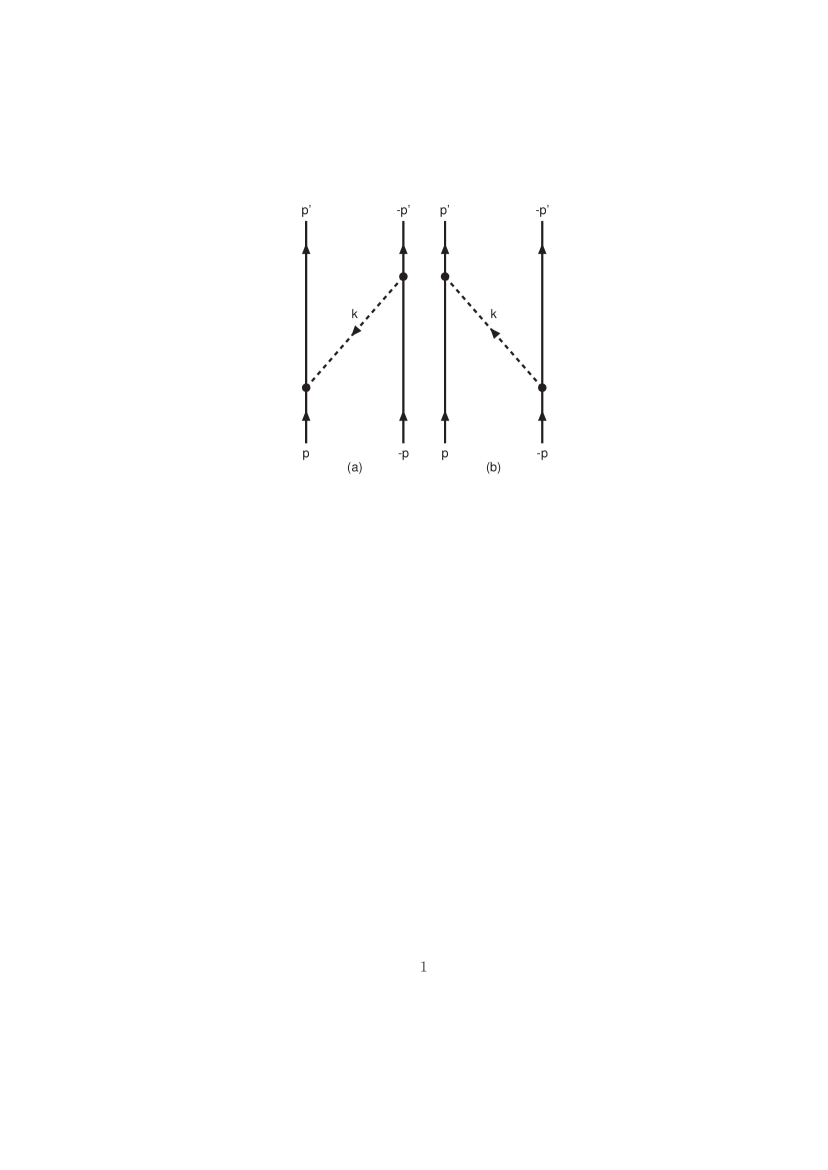
Figure 1: One-boson-exchange graphs: The dashed lines with momentum ${\bf k}$ refers to the bosons: pseudoscalar, vector, axial-vector, or scalar mesons.

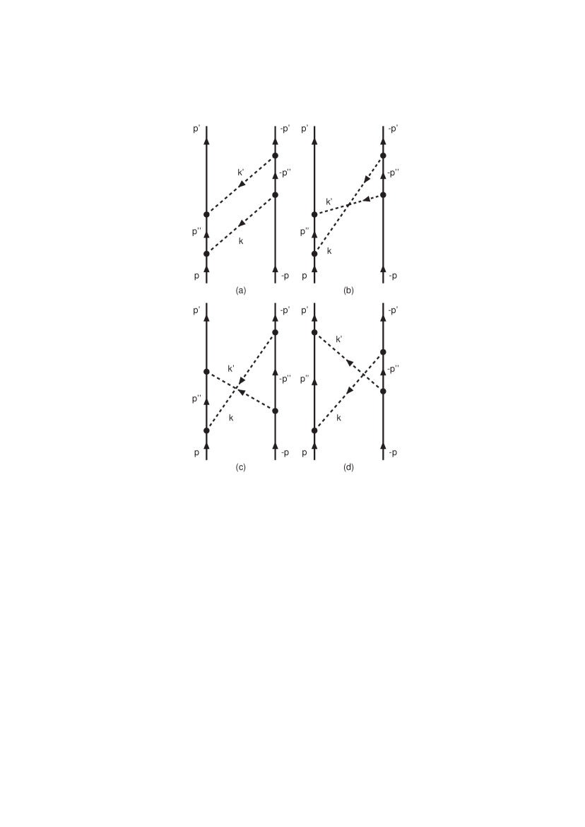
Figure 2: BW two-meson-exchange graphs: (a) planar and (b)-(d) crossed box. The dashed line with momentum ${\bf k}$ refers to the pion and the dashed line with momentum ${\bf k}^{\prime}$ refers to one of the other (vector, scalar, or pseudoscalar) mesons. To these we have to add the “mirror” graphs, and the graphs where we interchange the two meson lines.

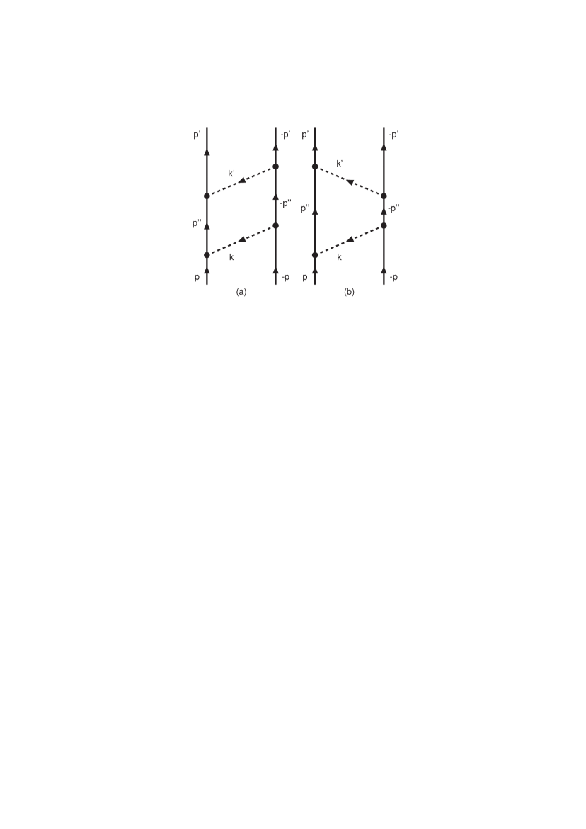
Figure 3: Planar-box TMO two-meson-exchange graphs. Same notation as in Fig. 2. To these we have to add the “mirror” graphs, and the graphs where we interchange the two meson lines.

The transformation of (23) to the Lippmann-Schwinger equation can be effectuated by defining

$$T({\bf p}^{\prime},{\bf p}) = N({\bf p}^{\prime})\ M({\bf p}^{\prime},{\bf p}|W)\ N({\bf p})\ ,$$ (25a)

$$V({\bf p}^{\prime},{\bf p}) = N({\bf p}^{\prime})\ K^{irr}({\bf p}^{\prime},{\bf p}|W)\ N({\bf p})\ ,$$ (25b)

where the transformation function is

$$N({\bf p})=\sqrt{\frac{{\bf p}_{i}^{2}-{\bf p}^{2}}{2M_{N}(E\left({\bf p}_{i})-E({\bf p})\right)}}\ .$$ (26)

Application of this transformation, yields the Lippmann-Schwinger equation

$$T({\bf p}^{\prime},{\bf p}) = V({\bf p}^{\prime},{\bf p})+\int\frac{d^{3}p^{\prime\prime}}{(2\pi)^{3}}$$ (27)

$$\times V({\bf p}^{\prime},{\bf p}^{\prime\prime})\ g({\bf p}^{\prime\prime};W)\;T({\bf p}^{\prime\prime},{\bf p})$$

with the standard Green function

$$g({\bf p};W)=\frac{M_{N}}{{\bf p}_{i}^{2}-{\bf p}^{2}+i\delta}\ .$$ (28)

The corrections to the approximation $E_{2}^{(+)}\approx g({\bf p};W)$ are of order $1/M^{2}$, which we neglect hencforth.

The transition from Dirac-spinors to Pauli-spinors, is given in Appendix C of Rij91 , where we write for the the Lippmann-Schwinger equation in the 4-dimensional Pauli-spinor space

$${\cal T}({\bf p}^{\prime},{\bf p}) = {\cal V}({\bf p}^{\prime},{\bf p})+\int\frac{d^{3}p^{\prime\prime}}{(2\pi)^{3}}\$$ (29)

$$\times{\cal V}({\bf p}^{\prime},{\bf p}^{\prime\prime})\ g({\bf p}^{\prime\prime};W)\ {\cal T}({\bf p}^{\prime\prime},{\bf p})\ .$$

The ${\cal T}$-operator in Pauli spinor-space is defined by

$$\chi^{(a)\dagger}_{\sigma^{\prime}_{a}}\chi^{(b)\dagger}_{\sigma^{\prime}_{b}}\;{\cal T}({\bf p}^{\prime},{\bf p})\;\chi^{(a)}_{\sigma_{a}}\chi^{(b)}_{\sigma_{b}}=\bar{u}_{a}({\bf p}^{\prime},\sigma^{\prime}_{a})\bar{u}_{b}(-{\bf p}^{\prime},\sigma^{\prime}_{b})$$

$$\times\tilde{T}({\bf p}^{\prime},{\bf p})\;u_{a}({\bf p},\sigma_{a})u_{b}(-{\bf p},\sigma_{b})\ .$$ (30)

and similarly for the ${\cal V}$-operator. Like in the derivation of the OBE-potentials NRS78 ; NRS77 we make off-shell and on-shell the approximation, $E({\bf p})=M+{\bf p}^{2}/2M$ and $W=2\sqrt{{\bf p}_{i}^{2}+M^{2}}=2M+{\bf p}_{i}^{2}/M$ , everywhere in the interaction kernels, which, of course, is fully justified for low energies only. In contrast to these kind of approximations, of course the full ${\bf k}^{2}$-dependence of the form factors is kept throughout the derivation of the TME. Notice that the Gaussian form factors suppress the high momentum transfers strongly. This means that the contribution to the potentials from intermediate states which are far off-energy-shell can not be very large.

Because of rotational invariance and parity conservation, the ${\cal T}$-matrix, which is a $4\times 4$-matrix in Pauli-spinor space, can be expanded into the following set of in general 8 spinor invariants, see for example SNRV71 . Introducing notation1

$${\bf q}=\frac{1}{2}({\bf p}^{\prime}+{\bf p})\ ,\ {\bf k}={\bf p}^{\prime}-{\bf p}\ ,\ {\bf n}={\bf p}\times{\bf p}^{\prime}\ ,$$ (31)

with, of course, ${\bf n}={\bf q}\times{\bf k}$, we choose for the operators $P_{j}$ in spin-space

$$P_{1} = 1\ ,$$ (32a)

$$P_{2} = \mbox{\boldmath$\sigma$}_{1}\cdot\mbox{\boldmath$\sigma$}_{2}\ ,$$ (32b)

$$P_{3} = (\mbox{\boldmath$\sigma$}_{1}\cdot{\bf k})(\mbox{\boldmath$\sigma$}_{2}\cdot{\bf k})-\frac{1}{3}(\mbox{\boldmath$\sigma$}_{1}\cdot\mbox{\boldmath$\sigma$}_{2})\ {\bf k}^{2}\ ,$$ (32c)

$$P_{4} = \frac{i}{2}(\mbox{\boldmath$\sigma$}_{1}+\mbox{\boldmath$\sigma$}_{2})\cdot{\bf n}\ ,$$ (32d)

$$P_{5} = (\mbox{\boldmath$\sigma$}_{1}\cdot{\bf n})(\mbox{\boldmath$\sigma$}_{2}\cdot{\bf n})\ ,$$ (32e)

$$P_{6} = \frac{i}{2}(\mbox{\boldmath$\sigma$}_{1}-\mbox{\boldmath$\sigma$}_{2})\cdot{\bf n}\ ,$$ (32f)

$$P_{7} = (\mbox{\boldmath$\sigma$}_{1}\cdot{\bf q})(\mbox{\boldmath$\sigma$}_{2}\cdot{\bf k})+(\mbox{\boldmath$\sigma$}_{1}\cdot{\bf k})(\mbox{\boldmath$\sigma$}_{2}\cdot{\bf q})\ ,$$ (32g)

$$P_{8} = (\mbox{\boldmath$\sigma$}_{1}\cdot{\bf q})(\mbox{\boldmath$\sigma$}_{2}\cdot{\bf k})-(\mbox{\boldmath$\sigma$}_{1}\cdot{\bf k})(\mbox{\boldmath$\sigma$}_{2}\cdot{\bf q})\ .$$ (32h)

Here we follow MRS89 , where in contrast to NRS78 , we have chosen $P_{3}$ to be a purely ‘tensor-force’ operator. The expansion in spinor-invariants reads

$${\cal T}({\bf p}^{\prime},{\bf p})=\sum_{j=1}^{8}\ \widetilde{T}_{j}({\bf p}^{\prime 2},{\bf p}^{2},{\bf p}^{\prime}\cdot{\bf p})\ P_{j}({\bf p}^{\prime},{\bf p})\ .$$ (33)

Similarly to (33) we expand the potentials $V$. Again following MRS89 , we neglect the potential forms $P_{7}$ and $P_{8}$, and also the dependence of the potentials on ${\bf k}\cdot{\bf q}$ . Then, the expansion (33) reads for the potentials as follows

$${\cal V}=\sum_{j=1}^{4}\tilde{V}_{j}({\bf k}\,^{2},{\bf q}\,^{2})\ P_{j}({\bf k},{\bf q})\ .$$ (34)

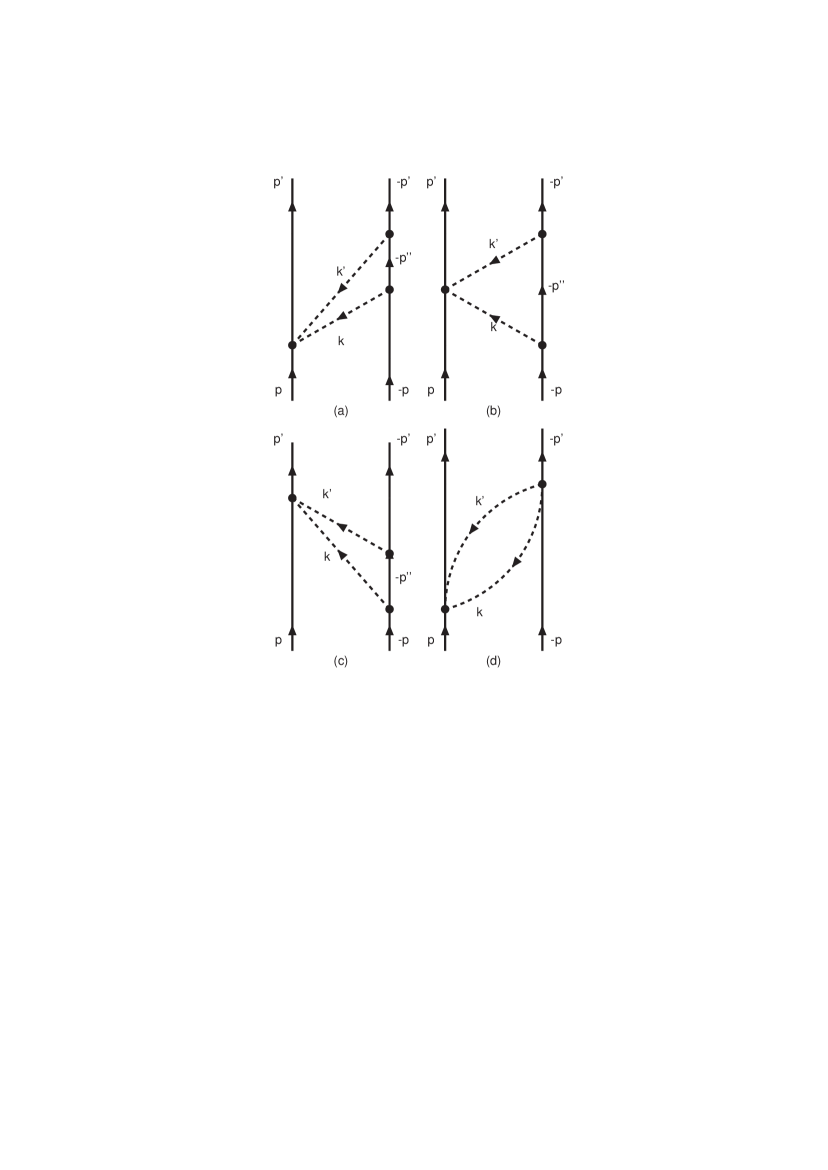
Figure 4: One- and Two-Pair exchange graphs. To these we have to add the “mirror” graphs, and the graphs where we interchange the two meson lines.

III Extended-Soft-Core Potentials in Momentum Space

The potential of the ESC-model contains the contributions from (i) one-boson-exchanges, Fig. 1, (ii) uncorrelated two-pseudoscalar-exchange, Fig. 2 and Fig. 3, and (iii) meson-pair-exchange, Fig 4. In this section we review the potentials and indicate the changes with respect to earlier papers on the OBE- and ESC-models.

III.1 One-Boson-Exchange Interactions in Momentum Space

The OBE-potentials are the same as given in NRS78 ; MRS89 , with the exception of (i) the zero in the scalar form factor, and (ii) the axial-vector-meson potentials. Here, we review the OBE-potentials briefly, and give those potentials that are not incuded in the above references. The local interaction Hamilton densities for the different couplings are

a) Pseudoscalar-meson exchange

$${\cal H}_{PV}=i\frac{f_{P}}{m_{\pi^{+}}}\bar{\psi}\gamma_{\mu}\gamma_{5}\psi\partial^{\mu}\phi_{P}\ ,$$ (35)

b) Vector-meson exchange

$${\cal H}_{V}=ig_{V}\bar{\psi}\gamma_{\mu}\psi\phi_{V}^{\mu}+\frac{f_{V}}{4{\cal M}}\bar{\psi}\sigma_{\mu\nu}\psi(\partial^{\mu}\phi^{\nu}_{V}-\partial^{\nu}\phi^{\mu}_{V})\ ,$$ (36)

c) Axial-vector-meson exchange

$${\cal H}_{A}=g_{A}\bar{\psi}\gamma_{\mu}\gamma_{5}\psi\phi_{A}^{\mu}+\frac{if_{A}}{{\cal M}}\left[\bar{\psi}\gamma_{5}\psi\right]\ \partial_{\mu}\phi^{\mu}_{A}\ ,$$ (37)

We take $f_{A}=0$, and notice that for the $A_{1}$-meson the interaction (37) is part of interaction

$${\cal L}_{I}^{(A)} = 2g_{A}\left[\bar{\psi}\gamma_{5}\gamma_{\mu}\frac{\mbox{\boldmath$\tau$}}{2}\psi+\left(\mbox{\boldmath$\pi$}\partial_{\mu}\sigma-\sigma\partial_{\mu}\mbox{\boldmath$\pi$}\right)\right.$$ (38)

$$\left.\vphantom{\frac{A}{A}}+f_{\pi}\partial_{\mu}\mbox{\boldmath$\pi$}\right]\cdot{\bf A}^{\mu}\ ,$$

which is such that the $A_{1}$ couples to an almost conserved axial current (PCAC). Therefore, the $A_{1}$-coupling used is compatible with broken ${\rm SU(2)}_{V}\times{\rm SU(2)}_{A}$-symmetry Schw69 .

d) Scalar-meson exchange

$${\cal H}_{S}=g_{S}\bar{\psi}\psi\phi_{S}\ .$$ (39)

Here, we used the conventions of BD65 where $\sigma_{\mu\nu}=[\gamma_{\mu},\gamma_{\nu}]/2i$. The scaling masses $m_{\pi^{+}}$ and ${\cal M}$ are chosen to be the charged pion and the proton mass, respectively. Note that the vertices for ‘diffractive’-exchange have the same Lorentz structure as those for scalar-meson-exchange.

Including form factors $f({\bf x}^{\prime}-{\bf x})$ , the interaction hamiltonian densities are modified to

$$H_{X}({\bf x})=\int\!d^{3}x^{\prime}\,f({\bf x}^{\prime}-{\bf x}){\cal H}_{X}({\bf x}^{\prime})\ ,$$ (40)

for $X=PV,\ V$, $A$, $S$, or $D$. Because of the convolutive non-local form, the potentials in momentum space are the same as for point interactions, except that the coupling constants are multiplied by the Fourier transform of the form factors.

In the derivation of the $V_{i}$ we employ the same approximations as in NRS78 ; MRS89 , i.e.

1. We expand in $1/M$: $E(p)=\left[{\bf k}^{2}/4+{\bf q}^{2}+M^{2}\right]^{\frac{1}{2}}$
   $\approx M+{\bf k}^{2}/8M+{\bf q}^{2}/2M$ and keep only terms up to first order in ${\bf k}^{2}/M$ and ${\bf q}^{2}/M$. This except for the form factors where the full ${\bf k}^{2}$-dependence is kept throughout the calculations. Notice that the gaussian form factors suppress the high ${\bf k}^{2}$-contributions strongly.

2. In the meson propagators $(-(p_{1}-p_{3})^{2}+m^{2})\approx({\bf k}^{2}+m^{2})$ .

3. When two different baryons are involved at a BBM-vertex their average mass is used in the potentials and the non-zero component of the momentum transfer is accounted for by using an effective mass in the meson propagator (for details see MRS89 ).

Due to the approximations we get only a linear dependence on ${\bf q}^{2}$ for $V_{1}$. In the following, we write

$$V_{i}({\bf k}^{2},{\bf q}^{2})=V_{ia}({\bf k}^{2})+V_{ib}({\bf k}^{2}){\bf q}^{2}\ ,$$ (41)

where in principle $i=1,8$.

The OBE-potentials are now obtained in the standard way (see e.g. NRS78 ; MRS89 ) by evaluating the BB-interaction in Born-approximation. We write the potentials $V_{i}$ of Eqs. (34) and (41) in the form

$$V_{i}({\bf k}\,^{2},{\bf q}\,^{2})=\sum_{X}\Omega^{(X)}_{i}({\bf k}\,^{2})\cdot\Delta^{(X)}({\bf k}^{2},m^{2},\Lambda^{2})\ ,$$ (42)

where $X=P,\ V,\ A,\ S$, and $D$ ($P=$ pseudoscalar, $V=$ vector, $A=$ axial-vector, $S=$ scalar, and $D=$ diffractive). Furthermore for $X=P,V$

$$\Delta^{(X)}({\bf k}^{2},m^{2},\Lambda^{2})=e^{-{\bf k}^{2}/\Lambda^{2}}/\left({\bf k}^{2}+m^{2}\right)\ ,$$ (43)

and for $X=S,A$ a zero in the form factor

$$\Delta^{(S)}({\bf k}^{2},m^{2},\Lambda^{2})=\left(1-{\bf k}^{2}/U^{2}\right)\ e^{-{\bf k}^{2}/\Lambda^{2}}/\left({\bf k}^{2}+m^{2}\right)\ ,$$ (44)

and for $X=D$

$$\Delta^{(D)}({\bf k}^{2},m^{2},\Lambda^{2})=\frac{1}{{\cal M}^{2}}e^{-{\bf k}^{2}/(4m_{P}^{2})}\ .$$ (45)

In the latter expression ${\cal M}$ is a universal scaling mass, which is again taken to be the proton mass. The mass parameter $m_{P}$ controls the ${\bf k}^{2}$-dependence of the pomeron-, $f$-, $f^{\prime}$-, $A_{2}$-, and $K^{\star\star}$-potentials.

Next, we make remarks which point out the differences in the potentials of this work as compared to with earlier soft-core model papers:

a) For pseudoscalar mesons, the graph’s of Fig. 1 give for the second-order potential $V_{PS}({\bf k},{\bf q})\approx K^{(2)}_{PS}({\bf p}^{\prime},{\bf p}|W)$

$$V_{PS}({\bf k},{\bf q}) = -\frac{f_{13}f_{24}}{m_{\pi}^{2}}\ \left(1-\frac{({\bf q}^{2}+{\bf k}^{2}/4)}{2M_{Y}M_{N}}\right)\cdot$$ (46)

$$\times\frac{(\mbox{\boldmath$\sigma$}_{1}\cdot{\bf k})(\mbox{\boldmath$\sigma$}_{2}\cdot{\bf k})}{\omega({\bf k})[\omega({\bf k})+a]}\ \exp\left(-{\bf k}^{2}/\Lambda^{2}\right)\ ,$$

where $a\approx\left({\bf q}^{2}+{\bf k}^{2}/4\right)-p_{i}^{2}$. Here, $p_{i}$ is the on-energy-shell momentum. On-energy-shell $a=0$, and henceforth we neglect the non-adiabatic effects, i.e. $a\neq 0$, in the OBE-potentials. However, we do include the non-local term in (46, to which we refer in the following as the Graz-correction Graz78 . From (46) we find for $\Omega^{(P)}_{i}$:

$$\Omega^{(P)}_{2a} = g^{P}_{13}g^{P}_{24}\left(\frac{{\bf k}^{2}}{12M_{Y}M_{N}}\right)$$ (47a)

$$\Omega^{(P)}_{2b} = -g^{P}_{13}g^{P}_{24}\left(\frac{{\bf k}^{2}}{24M_{Y}^{2}M_{N}^{2}}\right)$$ (47b)

$$\Omega^{(P)}_{3a} = -g^{P}_{13}g^{P}_{24}\left(\frac{1}{4M_{Y}M_{N}}\right)$$ (47c)

$$\Omega^{(P)}_{3a} = +g^{P}_{13}g^{P}_{24}\left(\frac{1}{8M_{Y}^{2}M_{N}^{2}}\right)$$ (47d)

The $\Omega^{(P)}_{2b,3b}$ contributions were not included in NRS78 ; MRS89 .

b) For vector-, and diffractive OBE-exchange we refer the reader to Ref. MRS89 , where the contributions to the different $\Omega^{(X)}_{i}$’s for baryon-baryon scattering are given in detail. Also, it is trivial to obtain from MRS89 the scalar-meson $\Omega_{i}$ making the substitutions:

$$\Omega^{(S)}_{i}\rightarrow\left(1-{\bf k}^{2}/U^{2}\right)\ \Omega^{(S)}_{i}\ ,$$

which now evidently have a zero for ${\bf k}^{2}=U^{2}$.
c) For the axial-vector mesons, the detailed derivation of the $\Omega_{i}^{(A)}$ is given in Appendix A. Using the approximations (1-5), from the $1^{st}$-term in the axial-meson propagator we get, see (71), the following contributions

$$\Omega^{(A)}_{2a} = -g^{A}_{13}g^{A}_{24}\left(1+\frac{{\bf k}^{2}}{24M_{Y}M_{N}}\right)\ ,$$ (48a)

$$\Omega^{(A)}_{2b} = -g^{A}_{13}g^{A}_{24}\ \frac{1}{6M_{Y}M_{N}}\ ,$$ (48b)

$$\Omega^{(A)}_{3} = +g^{A}_{13}g^{A}_{24}\ \frac{3}{4M_{Y}M_{N}}\ ,$$ (48c)

$$\Omega^{(A)}_{4} = -g^{A}_{13}g^{A}_{24}\ \frac{1}{2M_{Y}M_{N}}\ ,$$ (48d)

$$\Omega^{(A)}_{6} = -g^{A}_{13}g^{A}_{24}\ \frac{(M_{N}^{2}-M_{Y}^{2})}{4M_{Y}^{2}M_{N}^{2}}\ .$$ (48e)

From the $2^{nd}$-term propagator we get, see (73),

$$\Omega^{(A)}_{2a} = -g^{A}_{13}g^{A}_{24}\left(1-\frac{{\bf k}^{2}}{8M_{Y}M_{N}}\right)\cdot\frac{{\bf k}^{2}}{3m^{2}}\ ,$$ (49a)

$$\Omega^{(A)}_{2b} = +g^{A}_{13}g^{A}_{24}\ \frac{1}{2M_{Y}M_{N}}\cdot\frac{{\bf k}^{2}}{3m^{2}}\ ,$$ (49b)

$$\Omega^{(A)}_{3a} = -g^{A}_{13}g^{A}_{24}\left(1-\frac{{\bf k}^{2}}{8M_{Y}M_{N}}\right)\cdot\frac{1}{m^{2}}\ ,$$ (49c)

$$\Omega^{(A)}_{3b} = +g^{A}_{13}g^{A}_{24}\ \frac{1}{2M_{Y}M_{N}}\cdot\frac{1}{m^{2}}\ .$$ (49d)

For the inclusion of the zero in the axial-vector meson form factor we also make here the changes

$$\Omega^{(A)}_{i}\rightarrow\left(1-{\bf k}^{2}/U^{2}\right)\ \Omega^{(A)}_{i}\ ,$$

with the same $U$-mass as used for the scalar mesons. The motivation for the inclusion of a zero in the form factor here is again motivated by the quark-model, because for the axial-vector mesons one has the configuration $Q\bar{Q}(^{3}P_{1})$.

As in Ref. MRS89 in the derivation of the expressions for $\Omega_{i}^{(A)}$, given above, $M_{Y}$ and $M_{N}$ denote the mean hyperon and nucleon mass, respectively $M_{Y}=(M_{1}+M_{3})/2$ and $M_{N}=(M_{2}+M_{4})/2$, and $m$ denotes the mass of the exchanged meson. Moreover, the approximation $1/M^{2}_{N}+1/M^{2}_{Y}\approx 2/M_{N}M_{Y},$ is used, which is rather good since the mass differences between the baryons are not large.

III.2 One-Boson-Exchange Interactions in Configuration Space

1. For $X=P$ the local configuration space potentials are given in Ref. MRS89 . Here, we give the non-local Graz- corrections. From the Fourier transform of the $\Omega^{(P)}_{2b,3b}$ contributions and (47d) we have

   $$\Delta V_{PS}(r) = \frac{f_{13}f_{24}}{4\pi}\cdot\frac{m^{3}}{m_{\pi}^{2}}\cdot\left\{\vphantom{\frac{A}{A}}\frac{1}{3}(\mbox{\boldmath$\sigma$}_{1}\cdot\mbox{\boldmath$\sigma$}_{2})\left(\nabla^{2}\phi_{C}^{1}+\phi_{C}^{1}\nabla^{2}\right)\right.$$ (50)

   $$\left.\vphantom{\frac{A}{A}}+\left(\nabla^{2}\phi_{T}^{0}\ S_{12}+\phi_{T}^{0}S_{12}\nabla^{2}\right)\right\}/(4M_{Y}M_{N})\ ,$$

   where $\phi_{C}^{0},\phi_{C}^{1},\phi_{T}^{0}$ are defined in NRS78 ; MRS89 , and are functions of $(m,r,\Lambda)$.

2. Again, for $X=V,D$ we refer to the configuration space potentials in Ref. MRS89 . For $X=S$ we give here the additional terms w.r.t. those in MRS89 , which are due to the zero in the scalar form factor. They are

   $$\Delta V_{S}(r)=-\frac{m}{4\pi}\ \frac{m^{2}}{U^{2}}\ \left[g^{S}_{13}g^{S}_{24}\left\{\left[\phi^{1}_{C}-\frac{m^{2}}{4M_{Y}M_{N}}\phi^{2}_{C}\right]+\frac{m^{2}}{2M_{Y}M_{N}}\phi^{1}_{SO}\ {\bf L}\cdot{\bf S}\right.\right.$$

   $$\left.\left.+\frac{m^{4}}{16M_{Y}^{2}M_{N}^{2}}\phi^{1}_{T}\ Q_{12}+\frac{m^{2}}{4M_{Y}M_{N}}\frac{M_{N}^{2}-M_{Y}^{2}}{M_{Y}M_{N}}\ \phi^{(1)}_{SO}\cdot\frac{1}{2}(\mbox{\boldmath$\sigma$}_{1}-\mbox{\boldmath$\sigma$}_{2})\cdot{\bf L}\right\}\right]\ .$$ (51)

3. For the axial-vector mesons, the configuration space potential corresponding to (48e) is

   $$V_{A}^{(1)}(r)=-\frac{g_{A}^{2}}{4\pi}\ m\left[\phi^{0}_{C}\ (\mbox{\boldmath$\sigma$}_{1}\cdot\mbox{\boldmath$\sigma$}_{2})-\frac{1}{12M_{Y}M_{N}}\left(\nabla^{2}\phi^{0}_{C}+\phi^{0}_{C}\nabla^{2}\right)(\mbox{\boldmath$\sigma$}_{1}\cdot\mbox{\boldmath$\sigma$}_{2})\right.$$

   $$\left.\hskip 39.83368pt+\frac{3m^{2}}{4M_{Y}M_{N}}\ \phi^{0}_{T}\ S_{12}+\frac{m^{2}}{2M_{Y}M_{N}}\ \phi^{0}_{SO}(m,r)\ {\bf L}\cdot{\bf S}\right.$$

   $$\left.\hskip 39.83368pt+\frac{m^{2}}{4M_{Y}M_{N}}\frac{M_{N}^{2}-M_{Y}^{2}}{M_{Y}M_{N}}\ \phi^{(0)}_{SO}\cdot\frac{1}{2}(\mbox{\boldmath$\sigma$}_{1}-\mbox{\boldmath$\sigma$}_{2})\cdot{\bf L}\right]\ .$$ (52)

   The configuration space potential corresponding to (49d) is

   $$V_{A}^{(2)}(r) = \frac{g_{A}^{2}}{4\pi}\ m\ \left[\frac{1}{3}(\mbox{\boldmath$\sigma$}_{1}\cdot\mbox{\boldmath$\sigma$}_{2})\phi^{1}_{C}+\frac{1}{12M_{Y}M_{N}}((\mbox{\boldmath$\sigma$}_{1}\cdot\mbox{\boldmath$\sigma$}_{2})\left(\nabla^{2}\phi^{1}_{C}+\phi^{1}_{C}\nabla^{2}\right)\right.$$ (53)

   $$\left.+S_{12}\ \phi^{0}_{T}+\frac{1}{4M_{Y}M_{N}}\left(\nabla^{2}\phi^{0}_{T}S_{12}+\phi^{0}_{T}S_{12}\nabla^{2}\right)\right]\ ,$$

   The extra contribution to the potentials coming from the zero in the axial-vector meson form factor are obtained from the expression (52) by making substitutions as follows

   $$\Delta V_{A}^{(1)}(r) = V_{A}^{(1)}\left(\phi_{C}^{0}\rightarrow\phi_{C}^{1},\phi_{T}^{0}\rightarrow\phi_{T}^{1},\phi_{SO}^{0}\rightarrow\phi_{SO}^{1}\right)\cdot\frac{m^{2}}{U^{2}}\ .$$ (54)

   Note that we do not include the similar $\Delta V_{A}^{(2)}(r)$ since they involve ${\bf k}^{4}$-terms in momentum-space.

III.3 PS-PS-exchange Interactions in Configuration Space

In Fig. 2 and Fig. 3 the included two-meson exchange graphs are shown schematically. The Bruckner-Watson (BW) graphs Bru53 contain in all three intermediate states both mesons and nucleons. The Taketani-Machida-Ohnuma (TMO) graphs Tak52 have one intermediate state with only nucleons. Explicit expression for $K^{irr}(BW)$ and $K^{irr}(TMO)$ were derived Rij91 , where also the terminology BW and TMO is explained. The TPS-potentials for nucleon-nucleon have been given in detail in RS96a . The generalization to baryon-baryon is similar to that for the OBE-potentials. So, we substitute $M\rightarrow\sqrt{M_{Y}M_{N}}$, and include all PS-PS possibilities with coupling constants as in the OBE-potentials. As compared to nucleon-nucleon in RS96a here we have included in addition the potentials with double K-exchange. The masses are the physical pseudoscalar meson masses. For the intermediate two-baryon states we take into account of the different thresholds. We have not included uncorrelated PS-vector, PS-scalar, or PS-diffractive exchange. This because the range of these potentials is similar to those of the vector-, scalar-, and axial-vector-potentials. Moreover, for potentially large potentials, in particularly those with scalar mesons involved, there will be very strong cancellations between the planar- and crossed-box contributions.

III.4 MPE-exchange Interactions

In Fig. 4 both the one-pair graphs and the two-pair graphs are shown. In this work we include only the one-pair graphs. The argument for neglecting the two-pair graph is to avoid some ’double-counting’. Viewing the pair-vertex as containing heavy-meson exchange means that the contributions from $\rho(750)$ and $\epsilon=f_{0}(760)$ to the two-pair graphs is already accounted for by our treatment of the broad $\rho$ and $\epsilon$ OBE-potential. For a more complete discussion of the physics behind MPE we refer to our previous papers Rij93 ; RS96b . The MPE-potentials for nucleon-nucleon have been given in RS96b . The generalization to baryon-baryon is similar to that for the TPS-potentials. For the intermediate two-baryon states we neglect the different two-baryon thresholds. This because, although in principle possible, it complicates the computation of the potentials considerably. The generalization of the pair-couplings to baryon-baryon is described in paper II RY04b , section III. Also here in $N\!N$, we have in addition to RS96b included the pair-potentials with $K\otimes K$-, $K\otimes K^{*}$-, and $K\otimes\kappa$-exchange. The convention for the MPE coupling constants is the same as in RS96b .

III.5 The Schrödinger equation with Non-local potential

The non-local potentials are of the central-, spin-spin, and tensor-type. The method of solution of the Schrödinger equation for nucleon-nucleon is described in NRS78 and Graz78 . Here, the non-local tensor is in momentum space of the form ${\bf q}^{2}\ \tilde{v}_{T}({\bf k})$. For a more general treatment of the non-local potentials see Rij98 .

IV ESC-couplings and the QPC-model

According to the Quark-Pair-Creation (QPC) model, in the ${}^{3}P_{0}$-version Mic69 , the baryon-baryon-meson couplings are given in terms of the quark-pair creation constant $\gamma_{M}$, and the radii of the (constituent) gaussian quark wave functions, by Yao73 ; Yao75

$$g_{BBM}(\mp) = 2\left(9\pi\right)^{1/4}\gamma_{M}\ X_{M}\left(I_{M},L_{M},S_{M},J_{M}\right)\ F^{(\mp)}_{M}\ ,$$

where $X_{M}(\ldots)$ is a isospin, spin etc. recoupling coefficient, and

$$F^{(-)} = \left(m_{M}R_{M}\right)^{3/2}\left(\frac{3R_{B}^{2}}{3R_{B}^{2}+R_{M}^{2}}\right)^{3/2}\left(\frac{4R_{B}^{2}+R_{M}^{2}}{3R_{B}^{2}+R_{M}^{2}}\right)\ ,$$

$$F^{(+)} = \left(m_{M}R_{M}\right)^{1/2}\left(\frac{3R_{B}^{2}}{3R_{B}^{2}+R_{M}^{2}}\right)^{3/2}\frac{4R_{M}^{2}}{(3R_{B}^{2}+R_{M}^{2})}$$

are coming from the overlap integrals. Here, the superscripts $\mp$ refer to the parity of the mesons $M$: $(-)$ for $J^{PC}=0^{+-},1^{--}$, and $(+)$ for $J^{PC}=0^{++},1^{++}$. The radii of the baryons, in this case nucleons, and the mesons are respectively denoted by $R_{B}$ and $R_{M}$.

The QPC(${}^{3}P_{0}$)-model gives several interesting relations, such as

$$\begin{array}[]{cccccccc}g_{\omega}&=&3g_{\rho}&,&g_{\epsilon}&=&3g_{a_{0}}&,\\ g_{a_{0}}&\approx&g_{\rho}&,&g_{\epsilon}&\approx&g_{\omega}&.\end{array}$$ (55)

We see here an interesting link between the vector-meson and the scalar-meson couplings, which is not totally surprising, because the scalar polarization-vector $\epsilon_{0}$ of the vector mesons in the quark-model is realized by a $Q\bar{Q}(^{3}P_{0})$-state. This is the same state as for the scalar mesons in the $Q\bar{Q}$-picture.

From $\rho\rightarrow e^{+}e^{-}$, employing the current-field-identities (C.F.I’s) one can derive, see for example Roy67 , the following relation with the QPC-model

$$f_{\rho}=\frac{m_{\rho}^{3/2}}{\sqrt{2}|\psi_{\rho}(0)|}\Leftrightarrow\gamma_{M}\left(\frac{2}{3\pi}\right)^{1/2}\frac{m_{\rho}^{3/2}}{|^{\prime}\psi_{\rho}(0)^{\prime}|}\ ,$$ (56)

which, neglecting the difference between the wave functions on the left and right hand side, gives for the pair creation constant $\gamma_{M}\rightarrow\gamma_{0}=\frac{1}{2}\sqrt{3\pi}=1.535$. However, since in the QPC-model gaussian wave functions are used, the $Q\bar{Q}$-potential is a harmonic-oscillator one. This does not account for the $1/r$-behavior, due to one-gluon-exchange (OGE), at short distance. This implies a OG-correction LP96 to the wave function, which gives for $\gamma_{M}$ Chai80

$$\gamma_{M}=\gamma_{0}\left(1-\frac{16}{3}\frac{\alpha(m_{M})}{\pi}\right)^{-1/2}\ .$$ (57)

In Table 1 $\gamma_{M}(\mu)$ is shown, using from PDG02 the parameterization

$$\alpha_{s}(\mu)=4\pi/\left(\beta_{0}\ln(\mu^{2}/\Lambda_{QCD}^{2})\right)\ ,$$ (58)

with $\Lambda_{QCD}=100$ MeV and $\beta_{0}=11-\frac{2}{3}n_{f}$ for $n_{f}=3$.

Table 1: Pair-creation constant $\gamma_{M}$ as function of $\alpha_{s}$.

$\mu$ [GeV]	$\alpha_{s}(\mu)$	$\gamma_{M}(\mu)$
$\infty$	0.00	1.535
80.0	0.10	1.685
35.0	0.20	1.889
1.05	0.30	2.191
0.55	0.40	2.710
0.40	0.50	3.94
0.35	0.55	5.96

From this table one sees that at the scale of $m_{M}\approx 1$ GeV a value $\gamma_{M}=2.19$ is reasonable. This value we will use later when comparing the QPC-model predictions and the ESC04-model coupling constants. As remarked in Chai80 the correction to $\gamma_{0}$ is not small, and therefore should be seen as an indication.
In Table 2 we show the ${}^{3}P_{0}$-model results and the values obtained in the ESC04-fit. In this table we fixed $\gamma_{M}=2.19$ for the vector-, scalar-, and axial-vector-mesons, for $R_{B}=0.54$ fm. This ’effective’ radius is choosen from Yao73 , where it was determined using the Regge slopes. Here, one has to realize that the QPC-predictions are kind of ”bare” couplings, which allows vertex corrections from meson-exchange. For the pseudoscalar, a different value has to be used, showing indeed some ’running’-behavior as expected from QCD. In Chai80 , for the decays $\rho,\epsilon\rightarrow 2\pi$ etc. it was found $\gamma_{\pi}=3.33$, whereas we need here $\gamma_{\pi}=4.84$. Of course, there are several ways to change this by, for example, using other ’effective’ meson-radii. For the mesonic decays of the charmonium states $\gamma_{\psi}=1.12$. One notices the similarity between the QPC(${}^{3}P_{0}$)-model predictions and the fitted couplings.

Table 2: ESC04 Couplings and ${}^{3}P_{0}$-Model Relations.

Meson	$r_{M}[{\it fm}]$	$X_{M}$	$\gamma_{M}$	${}^{3}P_{0}$	ESC04
$\pi(140)$	0.66	$5/6$	4.84	$f=0.26$	$f=0.26$
$\rho(770)$	0.66	$1$	2.19	$g=0.93$	$g=0.78$
$\omega(783)$	0.66	$3$	2.19	$g=2.86$	$g=3.12$
$a_{0}(962)$	0.66	$1$	2.19	$g=0.93$	$g=0.81$
$\epsilon(760)$	0.66	$3$	2.19	$g=2.47$	$g=2.87$
$a_{1}(1270)$	0.66	$5\sqrt{2}/6$	2.19	$g=2.51$	$g=2.42$

Finally, we notice that the Schwinger relation Sch68

$$g_{NNa_{1}} \approx \frac{m_{a_{1}}}{m_{\pi}}f_{NN\pi}\ ,$$ (59)

is also rather well satisfied, both in the QPC-model and the ESC04-fit.

V ESC-model , Results

V.1 Parameters and Nucleon-nucleon Fit

During the searches fitting the NN-data with the present ESC-model ESC04, it was found that the OBE-couplings could be constraint successfully using the ’naive’ QPC-predictions as a guidance Mic69 . Although these predictions, see section IV, are ’bare’ ones, we kept during the searches all OBE-couplings rather closely in the neighborhood of these predictions. Also, it appeared that we could either fix all $F/(F+D)$-ratios to those as suggested by the QPC-model, or apply the same strategy as for the OBE-couplings.

The meson nonets contain rm SU(3) octet and mixed octet-singlet members. We assign in principle cut-offs $\Lambda_{8}$ and $\Lambda_{1}$ to the octets and singlets respectively. However, because of the octet-singlet mixings for the $I=0$ members, and the use of the physical mesons in the potentials, we use $\Lambda_{1}$ for all $I=0$-mesons. We have as free cut-off parameters $(\Lambda^{P}_{8},\Lambda^{V}_{8},\Lambda^{S}_{8})$, and similarly a set for the singlets. For the axial-vector mesons we use a single cut-off $\Lambda^{A}$.

The treatment of the broad mesons $\rho$ and $\epsilon$ is the same as in the OBE-models NRS78 ; MRS89 . In this treatment a broad meson is approximated by two narrow mesons. The mass and width of the broad meson determines the masses $m_{1,2}$ and the weights $\beta_{1,2}$ of these narrow ones. For the $\rho$-meson the same parameters are used as in NRS78 ; MRS89 . However, for $\epsilon=f_{0}(760)$, assuming NRS78 $m_{\epsilon}=760$ MeV and $\Gamma_{\epsilon}=640$ MeV, the Bryan-Gersten parameters Bry72 are used: $m_{1}=496.39796$ MeV, $m_{2}=1365.59411$ MeV, and $\beta_{1}=0.21781,\beta_{2}=0.78219$.

The ’mass’ of the diffractive exchanges were all fixed to $m_{P}=309.1$ MeV.

Summarizing the parameters we have for NN:

1. QPC-constrained: $f_{NN\pi},f_{NN\eta^{\prime}},g_{NN\rho},g_{NN\omega}$,
   $f_{NN\rho},f_{NN\omega},g_{NNa_{1}},g_{a_{0}},g_{NN\epsilon},g_{NNA_{2}},g_{NNP}$,

2. Pair couplings: $g_{NN(\pi\pi)_{1}},f_{NN(\pi\pi)_{1}},g_{NN(\pi\rho)_{1}}$,
   $g_{NN\pi\omega},g_{NN\pi\eta},g_{NN\pi\epsilon}$,

3. Cut-off masses: $\Lambda_{8}^{P},\Lambda_{8}^{V},\Lambda_{8}^{S},\Lambda_{1}^{V},\Lambda_{1}^{S},\Lambda^{A}$.

The pair coupling $g_{NN(\pi\pi)_{0}}$ was kept fixed at a small, but otherwise arbitrary value.

Together with the fit to the 1993 Nijmegen representation of the $\chi^{2}$-hypersurface of the NN-scattering data below $T_{lab}=350$ MeV Sto93 , also some low-energy parameters were fitted: the np and nn scattering lengths and effective ranges for the ${}^{1}S_{0}$, and the binding energy of the deuteron $E_{B}$.

We obtained for the phase shifts a $\chi^{2}/N_{\rm data}=1.155$. The phase shifts are shown in Table’s 3 and 4, and also in Fig.’s 5-8. In Table 8 the distribution of the $\chi^{2}$ for ESC04 is shown for the ten energy bins used in the single-energy (s.e.) phase shift analysis, and compared with that of the updated partial-wave analysis Klo93 .

Figure 5: Solid line: proton-proton $I=1$ phase shifts (degrees), as a function of $T_{\rm lab}$(MeV), for the ESC04-model. The dashed line: the m.e. phases of the Nijmegen93 PW-analysis Sto93 . The black dots: the s.e. phases of the Nijmegen93 PW-analysis. The diamonds: Bugg s.e. Bugg92 .

Figure 6: Solid line: proton-proton $I=1$ phase shifts (degrees), as a function of $T_{\rm lab}$(MeV), for the ESC04-model. The dashed line: the m.e. phases of the Nijmegen93 PW-analysis Sto93 . The black dots: the s.e. phases of the Nijmegen93 PW-analysis. The diamonds: Bugg s.e. Bugg92 .

Figure 7: Solid line: neutron-proton $I=0$ phase shifts (degrees), as a function of $T_{\rm lab}$(MeV) for the ESC04-model. The dashed line: the m.e. phases of the Nijmegen93 PW-analysis Sto93 . The black dots: the s.e. phases of the Nijmegen93 PW-analysis. The diamonds: Bugg s.e. Bugg92 .

Figure 8: Solid line: neutron-proton $I=0$ phase shifts (degrees), as a function of $T_{\rm lab}$(MeV) for the ESC04-model. The dashed line: the m.e. phases of the Nijmegen93 PW-analysis Sto93 . The black dots: the s.e. phases of the Nijmegen93 PW-analysis. The diamonds: Bugg s.e. Bugg92 .

Table 3: ESC04 pp and np nuclear-bar phase shifts in degrees.

$T_{\rm lab}$	0.38	1	5	10	25
$\sharp$ data	144	68	103	290	352
$\Delta\chi^{2}$	20	38	17	34	12
${}^{1}S_{0}(np)$	54.58	61.89	63.04	59.13	49.66
${}^{1}S_{0}$	14.62	32.63	54.76	55.16	48.58
${}^{3}S_{1}$	159.38	147.76	118.21	102.66	80.76
$\epsilon_{1}$	0.03	0.11	0.67	1.14	1.72
${}^{3}P_{0}$	0.02	0.13	1.55	3.67	8.50
${}^{3}P_{1}$	-0.01	-0.08	-0.87	-1.98	-4.78
${}^{1}P_{1}$	-0.05	-0.19	-1.52	-3.12	-6.49
${}^{3}P_{2}$	0.00	0.01	0.22	0.66	2.49
$\epsilon_{2}$	-0.00	-0.00	-0.05	-0.19	-0.78
${}^{3}D_{1}$	0.00	-0.01	-0.19	-0.69	-2.85
${}^{3}D_{2}$	0.00	0.01	0.22	0.86	3.73
${}^{1}D_{2}$	0.00	0.00	0.04	0.16	0.68
${}^{3}D_{3}$	0.00	0.00	0.00	0.00	0.04
$\epsilon_{3}$	0.00	0.00	0.01	0.08	0.56
${}^{3}F_{2}$	0.00	0.00	0.00	0.01	0.10
${}^{3}F_{3}$	0.00	0.00	-0.00	-0.03	-0.22
${}^{1}F_{3}$	0.00	0.00	-0.01	-0.07	-0.42
${}^{3}F_{4}$	0.00	0.00	0.00	0.00	0.02
$\epsilon_{4}$	0.00	0.00	0.00	-0.00	-0.05

Table 4: ESC04 pp and np nuclear-bar phase shifts in degrees.

$T_{\rm lab}$	50	100	150	215	320
$\sharp$ data	572	399	676	756	954
$\Delta\chi^{2}$	118	29	114	137	337
${}^{1}S_{0}(np)$	38.81	24.24	13.80	3.27	-9.80
${}^{1}S_{0}$	38.77	24.71	14.42	3.97	-9.05
${}^{3}S_{1}$	63.03	43.79	31.66	20.27	6.93
$\epsilon_{1}$	1.96	2.18	2.50	3.08	4.21
${}^{3}P_{0}$	11.51	9.68	5.14	-1.13	-10.19
${}^{3}P_{1}$	-8.16	-13.22	-17.43	-22.24	-28.81
${}^{1}P_{1}$	-9.92	-14.65	-18.67	-22.37	-29.87
${}^{3}P_{2}$	5.78	10.94	14.09	16.26	17.28
$\epsilon_{2}$	-1.66	-2.63	-2.92	-2.77	-2.13
${}^{3}D_{1}$	-6.58	-12.67	-17.29	-21.90	-27.41
${}^{3}D_{2}$	8.97	17.20	22.06	24.92	25.15
${}^{1}D_{2}$	1.67	3.77	5.76	7.82	9.65
${}^{3}D_{3}$	0.27	1.28	2.53	3.94	5.24
$\epsilon_{3}$	1.62	3.52	4.87	6.01	6.93
${}^{3}F_{2}$	0.32	0.75	1.00	0.97	0.07
${}^{3}F_{3}$	-0.65	-1.42	-2.02	-2.65	-3.63
${}^{1}F_{3}$	-1.12	-2.18	-2.87	-3.56	-4.70
${}^{3}F_{4}$	0.11	0.46	0.95	1.67	2.84
$\epsilon_{4}$	-0.19	-0.51	-0.81	-1.11	-1.44
${}^{3}G_{3}$	-0.27	-0.99	-1.88	-3.10	-4.92
${}^{3}G_{4}$	0.72	2.14	3.56	5.20	7.29
${}^{1}G_{4}$	0.15	0.40	0.67	1.02	1.63
${}^{3}G_{5}$	-0.05	-0.19	-0.32	-0.42	-0.43
$\epsilon_{5}$	0.21	0.72	1.26	1.90	2.75

Table 5: ESC04 Low energy parameters: S-wave scattering lengths and effective ranges, deuteron binding energy $E_{B}$, and electric quadrupole $Q_{e}$.

	experimental data			ESC04
$a_{pp}(^{1}S_{0})$	-7.823	$\pm$	0.010	-7.770
$r_{pp}(^{1}S_{0})$	2.794	$\pm$	0.015	2.753
$a_{np}(^{1}S_{0})$	-23.715	$\pm$	0.015	-23.860
$r_{np}(^{1}S_{0})$	2.760	$\pm$	0.030	2.787
$a_{nn}(^{1}S_{0})$	-18.70	$\pm$	0.60	-18.63
$r_{nn}(^{1}S_{0})$	2.75	$\pm$	0.11	2.81
$a_{np}(^{3}S_{1})$	5.423	$\pm$	0.005	5.404
$r_{np}(^{3}S_{1})$	1.761	$\pm$	0.005	1.749
$E_{B}$	-2.224644	$\pm$	0.000046	-2.224933
$Q_{e}$	0.286	$\pm$	0.002	0.271

Table 6: Meson parameters employed in the potentials shown in Figs. 1 to 4. Coupling constants are at ${\bf k}^{2}=0$. An asterisk denotes that the coupling constant is not searched, but constrained via SU(3) or simply put to some value used in previous work. The used widths of the $\rho$ and $\varepsilon$ are 146 MeV and 640 MeV respectively.

meson	mass (MeV)	$g/\sqrt{4\pi}$	$f/\sqrt{4\pi}$	$\Lambda$ (MeV)
$\pi$	138.04		0.2621	829.90
$\eta$	548.80		0.1673∗	900.00
$\eta^{\prime}$	957.50		0.1802	900.00
$\rho$	770.00	0.7794	3.3166	782.38
$\omega$	783.90	3.1242	0.0712	890.23
$\phi$	1019.50	–0.6957	1.2686∗	890.23
$a_{1}$	1270.00	2.4230		968.23
$f_{1}$	1420.00	1.4708		968.23
$f_{1}^{\prime}$	1285.00	0.5981∗		968.23
$a_{0}$	962.00	0.8111		1161.27
$\varepsilon$	760.00	2.8730		1101.62
$f_{0}$	993.00	–0.9669		1101.62
$a_{2}$	309.10	0.0000
Pomeron	309.10	2.2031

Table 7: Pair-meson coupling constants employed in the ESC04 MPE-potentials. Coupling constants are at ${\bf k}^{2}=0$.

$J^{PC}$	SU(3)-irrep	$(\alpha\beta)$	$g/4\pi$	$f/4\pi$
$0^{++}$	$\{1\}$	$(\pi\pi)_{0}$	0.0000
$0^{++}$	,,	$(\sigma\sigma)$	—
$0^{++}$	$\{8\}_{s}$	$(\pi\eta)$	–0.440
$0^{++}$		$(\pi\eta^{\prime})$	—
$1^{--}$	$\{8\}_{a}$	$(\pi\pi)_{1}$	0.000	0.119
$1^{++}$	,,	$(\pi\rho)_{1}$	0.835
$1^{++}$	,,	$(\pi\sigma)$	0.022
$1^{++}$	,,	$(\pi P)$	0.0
$1^{+-}$	$\{8\}_{s}$	$(\pi\omega)$	–0.170

Table 8: $\chi^{2}$ and $\chi^{2}$ per datum at the ten energy bins for the Nijmegen93 partial-wave-analysis. $N_{\rm data}$ lists the number of data within each energy bin. The bottom line gives the results for the total $0-350$ MeV interval. The $\chi^{2}$-excess for the ESC model is denoted by $\Delta\chi^{2}$ and $\Delta\hat{\chi}^{2}$, respectively.

$T_{\rm lab}$	$\sharp$ data	$\chi_{0}^{2}$	$\Delta\chi^{2}$	$\hat{\chi}_{0}^{2}$	$\Delta\hat{\chi}^{2}$
0.383	144	137.5549	20.7	0.960	0.144
1	68	38.0187	52.4	0.560	0.771
5	103	82.2257	10.0	0.800	0.098
10	209	257.9946	27.5	1.234	0.095
25	352	272.1971	29.2	0.773	0.083
50	572	547.6727	141.1	0.957	0.247
100	399	382.4493	32.4	0.959	0.081
150	676	673.0548	85.5	0.996	0.127
215	756	754.5248	154.6	0.998	0.204
320	954	945.3772	350.5	0.991	0.367
Total	4233	4091.122	903.9	0.948	0.208

We emphasize that we use the single-energy (s.e.) phases and $\chi^{2}$-surfaces Klo93 only as a means to fit the NN-data. As stressed in Sto93 the Nijmegen s.e. phases have not much significance. The significant phases are the multi-energy (m.e.) ones, see the dashed lines in the figures. One notices that the central value of the s.e. phases do not correspond to the m.e. phases in general, illustrating that there has been a certain amount of noise fitting in the s.e. PW-analysis, see e.g. $\epsilon_{1}$ and ${}^{1}P_{1}$ at $T_{lab}=100$ MeV. The m.e. PW-analysis reaches $\chi^{2}/N_{\rm data}=0.99$, using 39 phenomenological parameters plus normalization parameters, in total more than 50 free parameters. The related phenomenological PW-potentials NijmI,II and Reid93 SKTS94 , with respectively 41, 47, and 50 parameters, all with $\chi^{2}/N_{\rm data}=1.03$. This should be compared to the ESC-model, which has $\chi^{2}/N_{\rm data}=1.155$ using 20 parameters. These are 11 QPC-constrained meson-nucleon-nucleon couplings, 6 meson-pair-nucleon-nucleon couplings, and 3 gaussian cut-off parameters. From the figures it is obvious that the ESC-model deviates from the m.e. PW-analysis at the highest energy for some partial waves. If we evaluate the $\chi^{2}$ for the first 9 energies only, we obtain $\chi^{2}/N_{\rm data}=1.10$.

In Table 5 the results for the low energy parameters are given. In order to discriminate between the ${}^{1}S_{0}$-wave for pp, np, and nn, we introduced some charge independence breaking by taking $g_{pp\rho}\neq g_{np\rho}\neq g_{nn\rho}$. With this device we fitted the difference between the ${}^{1}S_{0}({\it pp})$ and ${}^{1}S_{0}({\it np})$ phases, and the different scattering lengths and effective ranges as well. We found $g_{np\rho}=0.71,\ g_{nn\rho}=0.74$, which are not far from $g_{pp\rho}=0.78$, see Table 6.

For $a_{nn}(^{1}S_{0})$ we have used in the fitting the value from an investigation of the n-p and n-n final state interaction in the ${}^{2}H({\it n},{\it nnp})$ reaction at 13 MeV Gon99 . The value for $a_{\it nn}(^{1}S_{0})$ is still somewhat in discussion. Another recent determination Huh00 obtained e.g. $a_{\it nn}(^{1}S_{0})=-16.27\pm 0.40$ fm. Fitting with the latter value yields for the ESC04-model the value $-16.74$ fm. Then, the quality of the fit to the phase shift analysis is the same, with small changes to the parameters and phase shifts. For a discussion of the theoretical and experimental situation w.r.t. these low energy parameters, see also Mil90 .

V.2 Coupling Constants

In Table 6 we show the OBE-coupling constants and the gaussian cut-off’s $\Lambda$. The used $\alpha=:F/(F+D)$-ratio’s for the OBE-couplings are: pseudoscalar mesons $\alpha_{pv}=0.388$, vector mesons $\alpha_{V}^{e}=1.0,\alpha_{V}^{m}=0.387$, and scalar-mesons $\alpha_{S}=0.852$, which is computed using the physical $S^{*}=f_{0}(993)$ coupling etc.. In Table 7 we show the MPE-coupling constants. The used $\alpha=:F/(F+D)$-ratio’s for the MPE-couplings are: $(\pi\eta)$ etc. and $(\pi\omega)$ pairs $\alpha(\{8_{s}\})=1.0$, $(\pi\pi)_{1}$ etc. pairs $\alpha_{V}^{e}(\{8\}_{a})=1.0,\alpha_{V}^{m}(\{8\}_{a})=0.387$, $(\pi\rho)_{1}$ etc. pairs $\alpha_{A}(\{8\}_{a})=0.652$.

Unlike in RS96a ; RS96b , we did not fix pair couplings using a theoretical model, based on heavy-meson saturation and chiral-symmetry. So, in addition to the 14 parameters used in RS96a ; RS96b we now have 6 pair-coupling fit parameters. In Table 7 the fitted pair-couplings are given. Note that the $(\pi\pi)_{0}$-pair coupling gets contributions from the $\{1\}$ and the $\{8_{s}\}$ pairs as well, giving in total $g_{(\pi\pi)}=0.10$, which has the same sign as in RS96b . The $f_{(\pi\pi)_{1}}$-pair coupling has opposite sign as compared to RS96b . In a model with a more complex and realistic meson-dynamics SR97 this coupling is predicted as found in the present ESC-fit. The $(\pi\rho)_{1}$-coupling agrees nicely with $A_{1}$-saturation, see RS96b . We conclude that the pair-couplings are in general not well understood, and deserve more study.

The ESC-model described here is fully consistent with SU(3)-symmetry. For the full SU(3) contents of the pair interaction Hamiltonians we refer to paper II, section III. Here, one finds for example that $g_{(\pi\rho)_{1}}=g_{A_{8}VP}$, and besides $(\pi\rho)$-pairs one sees also that $(KK^{*}(I=1)$- and $KK^{*}(I=0)$-pairs contribute to the NN potentials. All $F/(F+D)$-ratio’s are taken fixed with heavy-meson saturation in mind, which implies that these ratios are $0.4$ or $1.0$ depending on the heavy-meson type. The approximation we have made in this paper is to neglect the baryon mass differences, i.e. we put $m_{\Lambda}=m_{\Sigma}=m_{N}$. This because we have not yet worked out the formulas for the inclusion of these mass differences, which is straightforward in principle.

VI Discussion and Conclusions

We mentioned that we do not include negative energy state contributions. It is assumed that a strong pair suppression is operative at low energies in view of the composite nature of the nucleons. This leaves us for the pseudoscalar mesons with two essential equivalent interactions: the direct and the derivative one. In expanding the $NN\pi$- etc. vertex in $1/M_{N}$ these two interactions differ in the $1/M^{2}_{N}$-terms, see RS96a equations (3.4) and (3.5). This gives the possibility to use instead of the interaction in (35) the linear combination

$${\cal H}_{ps} = \frac{1}{2}\left[(1-a_{PV})g_{NN\pi}\bar{\psi}i\gamma_{5}\mbox{\boldmath$\tau$}\psi\cdot\mbox{\boldmath$\pi$}+\right.$$ (60)

$$\left.a_{PV}(f_{NN\pi}/m_{\pi})\gamma_{\mu}\gamma_{5}\mbox{\boldmath$\tau$}\psi\cdot\partial^{\mu}\mbox{\boldmath$\pi$}\right]\ ,$$

where $g_{NN\pi}=(2M_{N}/m_{\pi})f_{NN\pi}$. In ESC04 we have fixed $a_{PV}=1$, i.e. a purely derivative coupling.

The presented ESC-model is successful in describing the NN-data, even in this QPC-constrained version. Allowing total freedom in the couplings and cut-off masses, and without fitting the low-energy parameters, we reached the lowest $\chi^{2}_{p.d.p.}=1.10$. However, in that case some couplings look rather artificial. With some less freedom, a typical fit with ESC-model has $\chi^{2}_{p.d.p.}=1.15$, see e.g. RPN02 . This means that by constraining the parameters rather strongly, In the present NN-model ESC04 we we reached $\chi^{2}_{p.d.p.}=1.155$, i.e. we have only an extra $\Delta\chi^{2}\approx 250$, showing the feasibility of the QPC-inspired couplings.

The gain of this is that we have physical motivated OBE-couplings etc.. We will see in the next paper of this series, where we study the $S=-1$ YN-channels, that this feature persists when we fit NN and YN simultaneously. Then, the advantage is that going to the $S=-2$ YN- and YY-channels, it is reasonable to believe that the predictions made for these channels are realistic ones. So far, there did not exist a realistic NN-model with sizeable axial-vector mesons couplings as predicted by Schwinger Sch68 . Also, the zero in the scalar form factor has moderated the $f_{0}(760)$-coupling such that it fits with the QPC-model.

A momentum space version of ESC04 is readily available, using the material in RPN02 . We only have to add the momentum space potentials for the axial-vector mesons, and the Graz-corrections Graz78 , which is rather straightforward.

Finally, the potentials of this paper are available on the Internet online .

Appendix A Axial-vector-meson coupling to nucleons

The coupling of the axial mesons ($J^{PC}=1^{++}$) to the nucleons is given by

$${\cal L}_{ANN} = g_{A}\left[\bar{\psi}\gamma_{5}\gamma_{\mu}\bm{\tau}\psi\right]\cdot{\bf A}^{\mu}+i\frac{f_{A}}{\cal M}\left[\bar{\psi}\gamma_{5}\bm{\tau}\psi\right]\cdot\partial_{\mu}{\bf A}^{\mu}$$ (61)

$$\approx g_{A}\left[\bar{\psi}\gamma_{5}\gamma_{\mu}\bm{\tau}\psi\right]\cdot{\bf A}^{\mu}$$

Here, ${\cal M}=1$ GeV is again a scaling mass. We note that with $f_{A}=0$ this coupling is part of the $A_{1}$-interaction to pions and nucleons

$${\cal L}_{I}=2g_{A}\left[\bar{\psi}\gamma_{5}\gamma_{\mu}\frac{1}{2}\bm{\tau}\psi+\left(\bm{\pi}\partial_{\mu}\sigma-\sigma\partial_{\mu}\bm{\pi}\right)+f_{\pi}\partial_{\mu}\bm{\pi}\right]\cdot{\bf A}^{\mu}\ ,\\$$

which is such that the $A_{1}$ couples to an almost conserved axial current (PCAC). Therefore, the $A_{1}$-coupling used here is compatible with broken ${\rm SU(2)}_{V}\times{\rm SU(2)}_{A}$-symmetry, see e.g. Schw69 ; Alf73 . For a more complete discussion of the $A_{1}$-couplings to baryons we refer to SR97 . The latter reveals that as far as the axial-nucleon-nucleon coupling is concerned it is indeed of the type indicated above.

In the Proca-formalism, for the axial-vector propagator enters the polarization-sum

$$\Pi^{\mu\nu}(k)=\sum_{\lambda}\epsilon^{\mu}(k,\lambda)\epsilon^{\nu}(k,\lambda)=-\eta^{\mu\nu}+k^{\mu}k^{\nu}/m^{2}$$ (62)

where $m$ denotes the mass of the axial meson and $\epsilon^{\mu}(k)$ the polarization vector. Because

$$\left[\bar{\psi}\gamma_{5}\gamma_{\mu}\psi\right]k^{\mu}k^{\nu}\left[\bar{\psi}\gamma_{5}\gamma_{\nu}\psi\right]=\left[-i\bar{\psi}\gamma_{5}\gamma_{\mu}k^{\mu}\psi\right]\left[+i\bar{\psi}\gamma_{5}\gamma_{\nu}k^{\nu}\psi\right]$$ (63)

the second term in the ’propagator’ gives potentials which exactly are of the form as those of pseudo-vector exchange. We note that these $\Gamma_{5}(p^{\prime},p)=\gamma_{5}\gamma\cdot k$-factors come from the $\partial^{\mu}$-derivative of the pseudo-vector baryon-current. Then,

$$\bar{u}(p^{\prime})\Gamma_{5}(p^{\prime},p)u(p)\approx i\left[\mbox{\boldmath$\sigma$}\cdot({\bf p-p^{\prime}})\right.$$

$$\left.\mp\frac{E({\bf p})-E({\bf p}^{\prime})}{2M}\ \mbox{\boldmath$\sigma$}\cdot({\bf p+p^{\prime}})\right]$$ (64)

in contrast to what is used in Rij91 , where in the $1/M$-term $\omega({\bf k})$ is taken, instead of the baryon energy difference. Notice that the second term in (64) is of order $1/M^{2}$ and moreover vanishes on energy-shell. Hence this term we neglect. We write

$$\tilde{V}_{A}=\tilde{V}_{A}^{(1)}+\tilde{V}_{A}^{(2)}\ ,$$ (65)

where $\tilde{V}_{A}^{(2)}=\tilde{V}_{PV}$ with $f_{PV}^{2}/m_{\pi}^{2}\rightarrow g_{A}^{2}/m^{2}$. The transformation to the Lippmann-Schwinger equation implies the potential

$$\tilde{\cal V}_{A}\cong\left(1-\frac{{\bf k}^{2}}{8M^{\prime}M}-\frac{{\bf q}^{2}}{2M^{\prime}M}\right)\tilde{V}_{A}$$ (66)

Below, $M^{\prime}=M_{N}$ and $M=M_{Y}$, which are the average nucleon mass or an average hyperon mass, depending on the baryon-baryon system.

A.1 ${\cal V}^{(1)}_{A}$-potential term

Restriction to terms which are at most of order $1/M^{2}$, we find for the potential in Pauli-spinor space for the Lippmann-Schwinger equation for $\tilde{\cal V}_{A}^{(1)}$ Note here that, especially for the anti-spin-orbit term, that $(M,\bm{\sigma}_{1})$ and $(M^{\prime},\bm{\sigma}_{2})$ go with line 1 respectively with line 2. Defining

$${\bf k}={\bf p^{\prime}}-{\bf p}\ ,\ {\bf q}=\frac{1}{2}({\bf p^{\prime}}+{\bf p})\ ,$$ (67)

and using moreover the approximation

$$\frac{1}{M^{2}}+\frac{1}{M^{\prime 2}}\approx\frac{2}{MM^{\prime}}\ ,$$ (68)

the potential ${\cal V}_{A}^{(1)}$ is given in momentum space by

$$\tilde{\cal V}_{A}^{(1)} = -g_{A}^{2}\left[\left(1+\frac{({\bf q}^{2}+{\bf k}^{2}/4)}{6M^{\prime}M}\right)\bm{\sigma}_{1}\cdot\bm{\sigma}_{2}\right.$$ (69)

$$\left.+\frac{2}{MM^{\prime}}\left((\bm{\sigma}_{1}\cdot{\bf q})(\bm{\sigma}_{2}\cdot{\bf q})-\frac{1}{3}{\bf q}^{2}\bm{\sigma}_{1}\cdot\bm{\sigma}_{2}\right)\right.$$

$$\left.-\frac{1}{4M^{\prime}M}\left((\bm{\sigma}_{1}\cdot{\bf k})(\bm{\sigma}_{2}\cdot{\bf k})-\frac{1}{3}{\bf k}^{2}\bm{\sigma}_{1}\cdot\bm{\sigma}_{2}\right)\right.$$

$$\left.+\left(\frac{1}{4M^{2}}-\frac{1}{4M^{\prime 2}}\right)\cdot\frac{i}{2}(\bm{\sigma}_{1}-\bm{\sigma}_{2})\cdot{\bf q}\times{\bf k}\right.$$

$$\left.+\frac{i}{4M^{\prime}M}(\bm{\sigma}_{1}+\bm{\sigma}_{2})\cdot{\bf q}\times{\bf k}\right]\cdot\left(\frac{1}{\omega^{2}}\right)\ ,$$

Now, for a complete treatment one has to deal with the non-local tensor. Although this can be done, see notes on non-local tensor potentials Rij98 , in this work we use an approximate treatment. We neglect the purely non-local tensor potential by making in (69) the substitution

$$\frac{1}{MM^{\prime}}\left((\bm{\sigma}_{1}\cdot{\bf q})(\bm{\sigma}_{2}\cdot{\bf q})-\frac{1}{3}{\bf q}^{2}\bm{\sigma}_{1}\cdot\bm{\sigma}_{2}\right)\rightarrow$$

$$-\frac{1}{4MM^{\prime}}\left((\bm{\sigma}_{1}\cdot{\bf k})(\bm{\sigma}_{2}\cdot{\bf k})-\frac{1}{3}{\bf k}^{2}\bm{\sigma}_{1}\cdot\bm{\sigma}_{2}\right)$$ (70)

leading to a potential with only a non-local spin-spin term. With this approximation, (69) becomes

$$\tilde{\cal V}_{A}^{(1)} = -g_{A}^{2}\left[\left(1+\frac{({\bf q}^{2}+{\bf k}^{2}/4)}{6M^{\prime}M}\right)\bm{\sigma}_{1}\cdot\bm{\sigma}_{2}\right.$$ (71)

$$\left.-\frac{3}{4M^{\prime}M}\left((\bm{\sigma}_{1}\cdot{\bf k})(\bm{\sigma}_{2}\cdot{\bf k})-\frac{1}{3}{\bf k}^{2}\bm{\sigma}_{1}\cdot\bm{\sigma}_{2}\right)\right.$$

$$\left.+\left(\frac{1}{4M^{2}}-\frac{1}{4M^{\prime 2}}\right)\cdot\frac{i}{2}(\bm{\sigma}_{1}-\bm{\sigma}_{2})\cdot{\bf q}\times{\bf k}\right.$$

$$\left.+\frac{i}{4M^{\prime}M}(\bm{\sigma}_{1}+\bm{\sigma}_{2})\cdot{\bf q}\times{\bf k}\right]\cdot\left(\frac{1}{\omega^{2}}\right)\ .$$

Then, we find in configuration space

$${\cal V}_{A}^{(1)}=-\frac{g_{A}^{2}}{4\pi}\ m\left[\phi^{0}_{C}(m,r)(\bm{\sigma}_{1}\cdot\bm{\sigma}_{2})\right.$$

$$\left.-\frac{1}{12M^{\prime}M}\left(\nabla^{2}\phi^{0}_{C}+\phi^{0}_{C}\nabla^{2}\right)(m,r)(\bm{\sigma}_{1}\cdot\bm{\sigma}_{2})\right.$$

$$\left.+\frac{3m^{2}}{4M^{\prime}M}\ \phi^{0}_{T}(m,r)\ S_{12}+\frac{m^{2}}{2M^{\prime}M}\ \phi^{0}_{SO}(m,r)\ {\bf L}\cdot{\bf S}\right.$$

$$\left.+\frac{m^{2}}{4M^{\prime}M}\frac{M^{\prime 2}-M^{2}}{M^{\prime}M}\ \phi^{(0)}_{SO}(m,r)\cdot\frac{1}{2}(\mbox{\boldmath$\sigma$}_{1}-\mbox{\boldmath$\sigma$}_{2})\cdot{\bf L}\right]\ .$$

(72)

A.2 ${\cal V}^{(2)}_{A}$-potential term

For the PV-type contributions we have Graz78

$$\tilde{\cal V}_{A}^{(2)} = -\frac{g_{A}^{2}}{m^{2}}\left(1-\frac{{\bf k}^{2}}{8M^{\prime}M}-\frac{{\bf q}^{2}}{2M^{\prime}M}\right)\cdot$$ (73)

$$\times(\mbox{\boldmath$\sigma$}_{1}\cdot{\bf k})(\mbox{\boldmath$\sigma$}_{2}\cdot{\bf k})\ \left(\frac{1}{\omega^{2}}\right)\ .$$

The corresponding potentials in configuration space are

$${\cal V}_{A}^{(2)} = \frac{g_{A}^{2}}{4\pi}\ m\ \left[\frac{1}{3}(\mbox{\boldmath$\sigma$}_{1}\cdot\mbox{\boldmath$\sigma$}_{2})\phi^{1}_{C}+\frac{1}{12M^{\prime}M}(\mbox{\boldmath$\sigma$}_{1}\cdot\mbox{\boldmath$\sigma$}_{2})\right.$$ (74)

$$\left.\left(\nabla^{2}\phi^{1}_{C}+\phi^{1}_{C}\nabla^{2}\right)+S_{12}\ \phi^{0}_{T}\right.$$

$$\left.+\frac{1}{4M^{\prime}M}\left(\nabla^{2}\phi^{0}_{T}S_{12}+\phi^{0}_{T}S_{12}\nabla^{2}\right)\right]\ ,$$