Nucleons, Nuclear Matter and Quark Matter: A unified NJL approach.

Abstract

We use an effective quark model to describe both hadronic matter and deconfined quark matter. By calculating the equations of state and the corresponding neutron star properties, we show that the internal properties of the nucleon have important implications for the properties of these systems.

PACS numbers: 12.39.Fe; 12.39.Ki; 21.65.+f; 97.60.Jd
Keywords: Effective quark theories, Diquark condensation, Phase transitions, Compact stars

1 Introduction

Several recent studies have shown the advantages of using composite nucleons in finite density calculations [1], [2], [3]. For example, in some models the saturation mechanism of the system can be related to how the structure of the nucleon changes with density [4]. While saturating nuclear systems can also be readily obtained using point-like nucleons [5], if one wishes to explore the transition to quark matter it is desirable to start with a description of the nucleon on the quark level. Although the nucleon is a complex object, some simplification arises by treating it as an interacting quark-diquark state in the Faddeev approach. It turns out that this picture of the nucleon has considerable appeal, both theoretical and observational. For example, it nicely reproduces the light baryon spectrum [7], while a calculation without diquark correlations predicts an abundance of missing resonances [8]. Indeed, the widespread consensus that quark pairing is favorable in high density quark matter [9], where perturbative QCD has some predictive power, lends support to the idea that diquark correlations within the nucleon are important too [6].

In this work we consider the possibility of a connection between the diquark correlations within the nucleon and the pairing of quarks anticipated in color superconducting quark matter. We work with the assumption of two flavors. At zero temperature and normal nuclear matter density strange quarks certainly do not feature in the dynamics of the system, so this is a reasonable starting point. At higher densities strangeness could play a role through the formation of hyperons, kaon condensates and/or strange quark matter, depending on which of these phase transitions is favored and in what sequence they appear with respect to density [10, 11, 12, 13] . Actually, there are numerous possibilities for quark pairing and condensation in high density matter, especially if strangeness is introduced. Although these ideas can all be investigated within the framework we are using, we wish to concentrate here on the question of whether a unified description of diquark interactions can be achieved for both the nuclear matter (NM) and quark matter (QM) phases. For this purpose, we consider the simplest possibility that two flavor hadronic matter goes directly to two flavor QM, using the Nambu-Jona-Lasinio (NJL) model to describe both phases. In NJL type models, it has been shown that the mass of the strange quark tends to inhibit the formation of strange QM in the density region relevant to compact stars [15, 16, 17, 18]. The possibility of pseudoscalar condensation is considered in Refs.[19, 20, 21, 22], and the competition between the pseudoscalar condensates and the two-flavor superconducting phase has also been examined [23], although this remains to be applied to the charge neutral equation of state.

The NJL model was originally developed to describe interactions between structureless nucleons [24]. It has been shown that this approach does not lead to nuclear stability [25, 26, 27]. The idea of the NJL model in its present form is to describe QCD at low energies by assuming point-like interactions between quarks. This approximation is justified by the fact that gluon degrees of freedom should be of relatively minor importance at low energies. Therefore it is sufficient to construct a model where the gluon interactions are “frozen in,” meaning they are only present implicitly through the couplings of the model. The general form of the NJL Lagrangian density is given by,

$${\cal L}_{NJL}=\bar{\psi}(i\mbox{$\!\not\!\partial$}-m)\psi+\sum_{\alpha}G_{\alpha}(\bar{\psi}\Gamma_{\alpha}\psi)^{2},$$ (1.1)

where $\bar{\psi}$ and $\psi$ are the quark fields, $m$ is the current quark mass and $G_{\alpha}$ are the coupling constants associated with the various interaction channels. The interaction Lagrangian density can be expressed in a variety of equivalent forms using Fierz transformations [28]. Here we decompose it into $\bar{q}q$ and $qq$ interaction terms as follows:

$${\cal L}^{\rm int}_{\rm NJL} = G_{\pi}(\bar{\psi}\psi)^{2}-G_{\pi}(\bar{\psi}\gamma_{5}\mathbb{\tau}\psi)^{2}$$ (1.2)

$$- G_{\omega}(\bar{\psi}\gamma^{\mu}\psi)^{2}-G_{\rho}(\bar{\psi}\gamma^{\mu}\mathbb{\tau}\psi)^{2}$$ (1.3)

$$+ G_{s}(\bar{\psi}\gamma_{5}C\tau_{2}\beta^{A}\bar{\psi}^{T})(\psi^{T}C^{-1}\gamma_{5}\tau_{2}\beta^{A}\psi)$$ (1.4)

$$+ G_{a}(\bar{\psi}\gamma_{\mu}C\mathbb{\tau}\tau_{2}\beta^{A}\bar{\psi}^{T})(\psi^{T}C^{-1}\gamma_{\mu}\tau_{2}\mathbb{\tau}\beta^{A}\psi)$$ (1.5)

In order of appearance the above terms correspond to the scalar, pseudoscalar, vector-isoscalar and vector-isovector $\overline{q}q$ interactions, and the last two terms correspond to the scalar and the axial vector diquark channels. The color matrices are given by $\beta^{A}=\sqrt{3/2}\,\lambda^{A}$ $(A=2,5,7)$, indicating that these are attractive, color anti-symmetric diquark channels. In the NM phase the diquark interactions will lead to color singlet nucleons, and in the QM phase to color superconducting pairs. Indeed, QCD supports the idea that there is a strong attraction in the color anti-symmetric flavor singlet scalar channel, leading to the formation of condensed scalar diquarks (the so called 2SC phase) [6]. In our model these condensed pairs should arise from the same interaction (1.4) as the scalar diquarks in the nucleon constructed in the Faddeev approach.

Because the NJL model is non-renormalizable, the model is only fully specified after the choice of regularization scheme [29]. In our work quark confinement is ensured mathematically through the introduction of a finite infra-red cut-off ($\Lambda_{\rm IR}$) in the proper time regularization scheme [21, 30]. In this method, the unphysical quark decay thresholds are eliminated [1], as also found in the Dyson-Schwinger approach [30]. Of course, in the deconfined phase the infra-red cut-off will be set to zero [31].

2 Nucleons and nuclear matter

To describe NM we first consider the nucleon and its internal degrees of freedom. Incorporating the quark substructure of the nucleon through the Faddeev approach will allow us to examine how the nucleon properties change with density. The homogeneous Faddeev equation for the vertex function $\Gamma_{N}$ in the nucleon channel $(J,T)=(1/2,1/2)$ has the form $\Gamma_{N}=Z\,\Pi_{N}\,\Gamma_{N}$, where $Z$ is the quark exchange kernel and $\Pi_{N}$ the product of the quark and diquark propagators [28]. For our present, finite density calculations we restrict ourselves to the static approximation [32], where the momentum dependence of the quark exchange kernel $Z$ is neglected and a static parameter, c is instead introduced to reproduce the main features of the exact Faddeev calculation [1]. Then $\Pi_{N}$ becomes effectively the quark-diquark bubble graph given by

$$\Pi^{ab}_{N}(p) = \int\frac{d^{4}k}{(2\pi)^{4}}\tau^{ab}(p-k)S(k)$$ (2.1)

$$= \int\frac{d^{4}k}{(2\pi)^{4}}\left({\tau_{s}(p-k)\atop 0}{0\atop\tau_{a}^{\mu\nu}(p-k)}\right)S(k),$$ (2.2)

where $\tau_{s}$ and $\tau^{\mu\nu}_{a}$ refer to the scalar and axial vector components of the diquark t-matrices respectively , and $S(k)$ is the constituent quark propagator. The nucleon mass follows from the requirement that the Faddeev kernel $K\equiv Z\,\Pi_{N}$ has eigenvalue 1. In a similar way the mass of the Delta resonance can be calculated from the pole position in the $(J,T)=(3/2,3/2)$ channel, where only the axial vector diquark contributes.

Here we wish to use a more accurate description of the nucleon and delta masses, including also the pion cloud contributions [35]. This will enable us to consider a quantitative comparison of the scalar pairing found in the confined and deconfined phases. We take into consideration the self-energy contributions corresponding to the $N\to N\pi\to N$ and $N\to\Delta\pi\to N$ processes for the nucleon and the $\Delta\to\Delta\pi\to\Delta$ and $\Delta\to N\pi\to\Delta$ processes for the $\Delta$ [35]. The corresponding self-energies are,

$$\Sigma_{N}=\sigma_{NN}^{\pi}+\sigma_{N\Delta}^{\pi}$$ (2.3)

$$\Sigma_{\Delta}=\sigma_{\Delta\Delta}^{\pi}+\sigma_{\Delta N}^{\pi},$$ (2.4)

where

$$\sigma_{BB^{\prime}}^{\pi}=\frac{-3\hskip 4.2679ptg_{A}^{2}}{16\pi^{2}f_{\pi}^{2}}c_{BB^{\prime}}\int_{0}^{\infty}dk\frac{k^{4}u^{2}(k)}{\omega(k)[\omega_{BB^{\prime}}+\omega(k)]}$$ (2.5)

where $\omega_{BB^{\prime}}=(M_{B}-M_{B^{\prime}})$ is the physical baryon mass splitting (e.g. $\omega_{N\Delta}=1232-939$ MeV), and $\omega(k)=\sqrt{k^{2}+m_{\pi}^{2}}$ is the intermediate pion energy. For the $\pi BB^{\prime}$ vertex we assume the phenomenological dipole form $u(k)=\Lambda^{4}/(\Lambda^{2}+k^{2})^{2}$. The coefficients $c_{BB^{\prime}}$ come from the standard SU(6) couplings (i.e. $c_{NN}=1$, $c_{N\Delta}=32/25$ [36]). The baryon masses including the pion loop contributions are then given by $M_{B}=M_{B}^{(0)}+\Sigma_{B}$, where $M_{B}^{(0)}$ are the “bare” masses which follow from the quark-diquark equation.

The size of the self-energy of the nucleon, $\Sigma_{N}$, is not precisely known. Calculations indicate it could be up to -400 MeV [36, 37, 38, 39]. In the present work $\Sigma_{N}$ is varied by changing the dipole cut-off, $\Lambda$, within physically acceptable limits, in order to investigate how the pion cloud of the nucleon influences the equation of state of the system.

The form of the effective potential in the mean field approximation has been derived for symmetric NM in Ref.[31], starting from the quark Lagrangian, Eq.(1.5), and using the hadronization method. For the present calculations the effective potential is extended to the isospin asymmetric case, because for neutron star matter charge neutrality and chemical equilibrium typically lead to an abundance of neutrons over protons. The effective potential can be written as follows:

$$V^{\rm NM}=V_{\rm vac}+V_{N}-\frac{\omega_{0}^{2}}{4G_{\omega}}-\frac{\rho_{0}^{2}}{4G_{\rho}}-\frac{\mu_{e}^{4}}{12\pi^{2}}\,,$$ (2.6)

where

$$V_{\rm vac} = 12i\int\frac{{\rm d}^{4}k}{(2\pi)^{4}}\,{\rm ln}\,\frac{k^{2}-M^{2}}{k^{2}-M_{0}^{2}}+\frac{(M-m)^{2}}{4G_{\pi}}-\frac{(M_{0}-m)^{2}}{4G_{\pi}}$$ (2.7)

is the vacuum term. The Fermi motion of the nucleons moving in the scalar and vector mean fields gives rise to the term

$$V_{N}=-2\sum_{\alpha={\rm p,n}}\int\frac{{\rm d}^{3}k}{(2\pi)^{3}}\,\Theta(k_{F_{\alpha}}-k)\left(\sqrt{k_{F_{\alpha}}^{2}+M_{N}^{2}(M)}-\sqrt{k^{2}+M_{N}^{2}(M)}\right)$$ (2.8)

where $M_{N}(M)$ is the nucleon mass in-medium, which is the sum of the bare mass and the pion cloud contribution. The relations between the chemical potentials, which are the variables of $V^{\rm NM}$, and the Fermi momenta appearing in Eq.(2.8) are given by

$$\mu_{n}=\sqrt{M_{N}^{2}+k_{F_{n}}^{2}}+3\omega_{0}-\rho_{0}$$ (2.9)

$$\mu_{p}=\sqrt{M_{N}^{2}+k_{F_{p}}^{2}}+3\omega_{0}+\rho_{0}$$ (2.10)

The constituent quark mass, $M$, and the mean vector fields ($\omega_{0}$ and $\rho_{0}$) in NM are determined by minimizing the effective potential for fixed chemical potentials . The chemical potential of the (massless) electron in the last term of (2.6) is fixed by the requirement of beta equilibrium as $\mu_{e}=\mu_{n}-\mu_{p}$.

For discussion of the phase structure of this model in Sect.5, we introduce the chemical potentials associated with baryon number and isospin:

$$\mu_{B}=\frac{1}{2}(\mu_{p}+\mu_{n});\hskip 28.45274pt\mu_{I}=\frac{1}{2}(\mu_{p}-\mu_{n}).$$ (2.11)

The parameters of the model are determined as follows. We choose $\Lambda_{\rm IR}=285$ MeV to be of the order of $\Lambda_{QCD}$. We calculate $\Lambda_{\rm UV}$, $m$ and $G_{\pi}$ so as to reproduce $f_{\pi}=93$ MeV (through the matrix element for pion decay), $m_{\pi}=140$ MeV (through the Bethe Salpeter equation for the pion) and constituent quark mass at zero density, $M_{0}=400$ MeV (via the gap equation). The resulting equation of state is not very sensitive to the initial choices of $\Lambda_{\rm IR}$ and $M_{0}$. The parameter $G_{\omega}$ is fixed to give the empirical binding energy per nucleon of symmetric NM ($E_{B}=17$ MeV), and the parameter $G_{\rho}$ is adjusted to the symmetry energy ($a_{4}=32$ MeV at $\rho_{0}=0.17$fm^-3). The coupling in the axial vector diquark channel, $G_{a}$, is fixed by the mass of the Delta, since in this case the scalar diquark channel does not contribute. Then the coupling in the scalar diquark channel, $G_{s}$, is in turn determined by the nucleon mass. For the static parameter in the quark exchange kernel we use $c=450$ MeV. This calculation of baryon masses is carried out for several initial choices of the dipole cut-off $\Lambda$, which controls the magnitude of the pion loop contributions to the nucleon mass, $\Sigma_{N}$. We will show the results for three different values of $\Lambda$, leading to $\Sigma_{N}=-200$ MeV, $-300$ MeV and $-400$ MeV. The resulting parameter sets are shown in Table 1. (The first set corresponds to the case where the nucleon and delta masses are reproduced without pion cloud contributions.)

$\Lambda$	$\Sigma_{N}$	$\Sigma_{\Delta}$	$r_{a}$	$r_{s}$	$r_{\omega}$	$r_{\rho}$
-	0	0	0.27	0.30	0.48	0.70
710	-200	-183	0.21	0.27	0.30	0.74
803	-300	-266	0.18	0.24	0.24	0.76
877	-400	-346	0.15	0.22	0.19	0.77

Table 1: Parameters corresponding to different choices of $\Sigma_{N}$. We define $r_{\alpha}=G_{\alpha}/G_{\pi}$ ($\alpha=a,s,\omega,\rho$). $\Lambda$, $\Sigma_{N}$ and $\Sigma_{\Delta}$ are in MeV.

The function $M_{N}(M)$, which is needed in (2.8) to minimize the effective potential for finite density, is calculated by assuming that the ratio $g_{A}/f_{\pi}$ in (2.5) is independent of density. This is supported by a recent analysis of the pion-nucleus optical potential [40], which has shown that the pion decay constant in nuclear matter is reduced by $20\%$, which is the same as the quenching of $g_{A}$ derived from Gamow-Teller matrix elements [41]. The pion mass in the medium is constrained by chiral symmetry which leads to the relation $m_{\pi}(\rho)^{2}=m_{\pi}^{2}\cdot M_{0}/M$. This small enhancement of the pion mass in the medium is taken into account in the calculation but its effect is not very important.

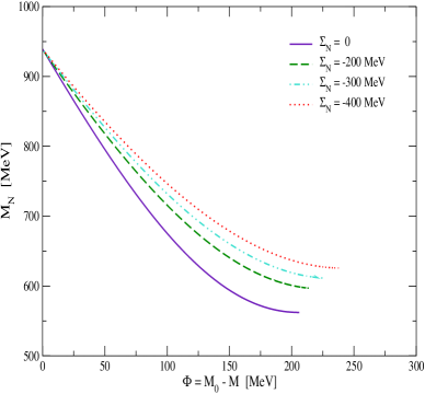
Figure 1: The mass of the nucleon as a function of the scalar potential ($\Phi=M_{0}-M$).

The relationship between the nucleon mass and the constituent quark mass for the four cases of Table 1 is shown in Fig.1. Note that in the region $M>200$ MeV, which is most relevant for normal densities, both the slopes and the curvatures of the lines decrease in magnitude as the attraction from the pion loop increases. Thus the inclusion of pion loop effects on the nucleon mass leads to a reduced effective $\sigma\,NN$ coupling and to a reduced scalar polarizability in the medium [1]. The self consistently calculated quark and nucleon masses are shown as functions of the density in Fig.2.

Concerning the pion exchange effects on the NM equation of state, we note that in addition to the term which can be incorporated into the nucleon mass there is also the familiar “Fock term” which originates from the Pauli principle. However this contribution is quite small when the short range correlations between nucleons in the spin-isospin channel are included [42], and will be neglected here for simplicity.

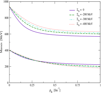
Figure 2: The effective masses of quarks (lower lines) and nucleons (upper lines) in the hadronic phase for several choices of the nucleon self-energy.

3 Quark matter

In the most simple mean field description of quark matter, each energy level for the quarks is filled up to the Fermi energy. At the Fermi surface, only a small attraction between quarks leads to the formation of Cooper pairs, analagous to the phenomenon of BCS pairing of electrons in a superconductor. In QCD we anticipate that color superconductivity will arise through the $\bar{3}_{c}$ channel, reducing the energy of the system through the condensation of color anti-symmetric pairs. The effective potential for QM thus has the form

$$V^{\rm QM}=V_{\rm vac}+V_{Q}+V_{\Delta}-\frac{\mu_{e}^{4}}{12\pi^{2}}$$ (3.1)

where the vacuum part, $V_{\rm vac}$, is the same as for NM (Eq. (2.7)) except that the infra-red cut-off is zero in QM. Furthermore,

$$V_{Q}=-6\sum_{\alpha={\rm u,d}}\int\frac{{\rm d}^{3}k}{(2\pi)^{3}}\,\Theta(\mu_{\alpha}-E_{Q}(k))\left(\mu_{\alpha}-E_{Q}(k)\right)$$ (3.2)

describes the Fermi motion of quarks with chemical potentials $\mu_{u}$ and $\mu_{d}$, and $E_{Q}(k)=\sqrt{M^{2}+k^{2}}$. The term (3.2) is analagous to $V_{N}$ in NM, except that the quark mass, $M$, corresponds directly to the scalar field in the system, i.e., there is no scalar polarizability of the quarks. The term $V_{\Delta}$ describes the effect of the pairing gap and is given by

$$V_{\Delta}=2i\int\frac{{\rm d}^{4}k}{(2\pi)^{4}}\sum_{\alpha=+,-}\Big{[}{\rm ln}\,\frac{k_{0}^{2}-(\epsilon_{\alpha}+\mu_{I})^{2}}{k_{0}^{2}-(E_{\alpha}+\mu_{I})^{2}}\\ +{\rm ln}\,\frac{k_{0}^{2}-(\epsilon_{\alpha}-\mu_{I})^{2}}{k_{0}^{2}-(E_{\alpha}-\mu_{I})^{2}}\Big{]}+\frac{\Delta^{2}}{6G_{s}}\,,$$ (3.3)

where $\epsilon_{\pm}(k)=\sqrt{(E_{Q}(k)\pm\mu_{B}/3)^{2}+\Delta^{2}}$, $E_{\pm}=|E_{Q}(k)\pm\mu_{B}/3|$, and we introduced the chemical potentials for baryon number and isospin

$$\mu_{B}=\frac{3}{2}(\mu_{u}+\mu_{d});\hskip 28.45274pt\mu_{I}=\frac{1}{2}(\mu_{u}-\mu_{d}),$$ (3.4)

which corresponds to (2.11) in the NM phase. The electron chemical potential is determined from beta equilibrium as $\mu_{e}=\mu_{d}-\mu_{u}=-2\mu_{I}$.

The gap $\Delta$ and the quark mass $M$ are determined by minimizing the effective potential for fixed chemical potentials. Our results, discussed below, show that $M$ is quite small in the QM phase, i.e., we have almost current quarks.

Note that the vector-type interactions are set to zero in QM, even though in the description of NM the vector mean fields are clearly important. This assumption, which has been made implicitly in almost all investigations of high density quark matter, is supported by the discussions of vector meson poles in Ref.[31]. It is also supported by recent arguments related to the EMC effect [45], which show that in the high energy region, where one has essentially current quarks (as in the present high density case), the mean vector field must indeed be set to zero.

In the following discussions, we distinguish the normal quark matter (NQM) phase, which is characterized by $\Delta=0$, from the color superconducting (SQM) phase ($\Delta>0$). Note that the value of $G_{s}=r_{s}G_{\pi}$ controls the outcome of this minimization through the last term in (3.3). In these calculations we focus on the case where the pairing strength ($r_{s}$) in QM takes the same value as in NM, namely the value required to obtain the correct nucleon mass after the pion cloud contribution is taken into account.

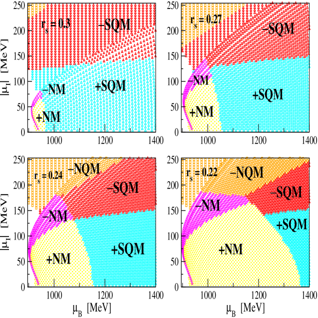
Figure 3: Phase Diagrams with $r_{s}(NM)=r_{s}(QM)$. The nucleon self-energies ($\Sigma_{N}$) are 0, -200, -300 and -400 MeV respectively. Note that in each region the sign of the charge density is indicated. Globally charge neutral matter occurs at the boundary of the positively and negatively charged regions.

4 Phase diagrams and mixed phases

To construct a phase diagram in the plane of the chemical potentials, as in Fig.3 which is discussed below, we compare the effective potentials for the NM, NQM and SQM phases at each point. The phase with the smallest effective potential (largest pressure) is the one which is physically realized. At each point we calculate the baryon and charge densities,

$$\rho_{B}^{a} = -\frac{\partial V^{a}}{\partial\mu_{B}}$$ (4.5)

$$\rho_{c}^{a} = -\frac{1}{2}(\frac{\partial V^{a}}{\partial\mu_{B}}+\frac{\partial V^{a}}{\partial\mu_{I}}),$$ (4.6)

where $a=$ NM, NQM or SQM. The actual equation of state as a function of baryon density is then constructed according to global charge neutrality. If charge neutrality can be realized within one phase (for example the NM phase), one simply moves along the charge neutral line in the phase diagram (for example the line +NM/-NM in Fig.3.) as the baryon density increases. When a phase transition occurs, it is necessary to construct a mixed phase, which is composed of positively and negatively charged components belonging to two different phases [46]. A charge neutral mixture of NM and QM (where QM refers to either NQM or SQM), for example, is characterized by the volume fraction,

$$\chi^{NM}=\frac{\rho_{c}^{QM}}{\rho_{c}^{QM}-\rho_{c}^{NM}}$$ (4.7)

which ranges from 0 to 1, as the density increases from the point of pure NM (where $\rho_{c}^{NM}=0$) to the one of pure QM (where $\rho_{c}^{QM}=0$).

The baryon and energy densities for the mixed phase are then expressed by the volume fraction as follows,

$$\rho_{B}^{M} = \chi^{NM}\rho_{B}^{NM}+(1-\chi^{NM})\rho_{B}^{QM}$$ (4.8)

$${\cal E}^{M} = \chi^{NM}{\cal E}^{NM}+(1-\chi^{NM}){\cal E}^{QM}$$ (4.9)

Note that the components of the mixed phase have equal pressures ($P^{M}=P^{NM}=P^{QM}$) at each point ($\mu_{B},\mu_{I}$) on the phase boundary. In this way one moves along the phase boundaries between NM and QM while $\rho_{B}$ is increasing, until one comes to the point where charge neutral pure QM is realized ($\chi^{NM}=0$)

In practice, our procedure is as follows. We first find the point where the effective potential for charge neutral NM becomes equal to the one for QM. At this point $\chi^{NM}=1$, since $\rho_{c}^{NM}=0$. From this point we incrementally increase either the neutron or proton density (depending on whether the transition is in the direction of increasing neutron and/or proton density). For example, the transition from NM to SQM ($r_{s}=0.27$) is in the direction of increasing neutron density. For each neutron density, we determine the value for proton density required to ensure that we are on the phase boundary. Next we calculate the charge densities of each phase and the resulting volume fraction. The volume averaged properties of the mixed phase are then related to its component phases by Eqns. (4.8) and (4.9). This process continues until we encounter the point where the QM phase becomes charge neutral ($\rho_{c}^{QM}=0$), and thus the volume fraction $\chi^{NM}$ goes to 0. From here the remainder of the equation of state will be the pure charge neutral QM phase.

5 Results

The equations of state for this model exhibit phase transitions from the confined quark-diquark states employed in the description of NM to a phase with condensed quark pairs in the form of color superconducting QM. The key point in our present work is to equate the pairing strength for the color superconducting pairs in QM with the scalar diquark interactions inside the nucleon. Depending on the amount of attractive contributions of the pion cloud to the nucleon mass, this gives rise to a series of phase diagrams shown in Fig.3, corresponding to the four cases of Table 1.

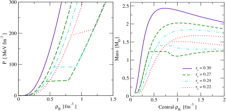
Figure 4: Equations of state and neutron star masses for the choices of scalar attraction described in the text.

The four diagrams in Fig.3 are shown for increasing pion cloud contributions to the nucleon mass, i.e., decreasing scalar diquark interactions characterized by the ratio $r_{s}$. Starting from the first diagram in Fig.3, the regions occupied by SQM become smaller while those of NM and NQM phases become larger. In the first phase diagram, where the pion cloud is not included and the whole attraction within the nucleon is attributed to the diquark correlations, the NM phase is expelled almost completely and overwhelmed by the SQM phase even in the low density region. Since this is clearly unphysical, we can conclude that the naive quark-diquark picture of the nucleon leads to a phase structure which is in conflict with empirical evidence. Hence some attraction within the nucleon must be attributed to the pion cloud.

The second diagram in Fig.3, which corresponds to a mass shift of $\Sigma_{N}=-200$ MeV from the pion cloud, involves a mixed phase -NM/+SQM before the system undergoes a transition to the pure SQM phase. The phase boundary in this case is rather short, indicating that the pressure is almost constant during the phase transition. In the third diagram ($\Sigma_{N}=-300$ MeV), the NM region extends to larger values of $\mu_{B}$, and the charge neutral phase boundary shrinks almost to a point. The fourth diagram ($\Sigma_{N}=-400$ MeV) involves a mixed phase +NM/-SQM before the pure SQM phase is reached.

The charge neutral equations of state for these four cases are shown on the left hand side of Fig.4. In the low density region ($0>\rho_{B}>0.001$ fm^-3) we use the equation of state of Negele and Vautherin [47] to describe the neutron star crust. On the NM side of Fig.4, the equation of state becomes softer with increasing pion cloud contributions, $\Sigma_{N}$. This can be understood from our discussions in Sect. 2. In particular, the inclusion of the pion cloud leads to a reduction of the effective $\sigma NN$ coupling in the medium, which must be balanced by a smaller vector coupling (the parameter $r_{\omega}$ in Table 1) in order to maintain the correct binding energy at the nuclear matter density $0.17$ fm^-3. Note that the actual saturation point for the model moves to somewhat higher densities (0.14, 0.19, 0.21 and 0.25 fm^-3) when $\Sigma_{N}$ increases (0, -200,-300 and -400 MeV respectively). As noted in earlier works the only parameter in the present model that may be adjusted to give the saturation point is $G_{\omega}$ [28]. With this in mind these results are reasonably close to the empirical value of $\rho_{0}=0.17$ fm^-3.

On the QM side all cases considered here give almost identical equations of state, indicating that the relationship between density and pressure in charge neutral SQM is not sensitive to the value of $r_{s}$ (or indeed to the value of $\Delta$). However, the transition densities are sensitive to $r_{s}$. In all cases considered here, the pressure variations in the mixed phase are rather small, indicating that our construction, based on the Gibbs criteria of phase equilibrium, gives similar results to a naive Maxwell construction between charge neutral NM and SQM.

Through the Tolman Oppenheimer Volkoff (TOV) equations [48] any equation of state specifies a unique set of non-rotating relativistic stars. The right hand side of Fig.4 illustrates the solutions to these equations for each of the equations of state on the left hand side of Fig.4. We see from these figures that the inclusion of pion cloud contributions to the nucleon mass, leading to a decreasing strength of scalar diquark pairing, has significant effects on the properties of neutron stars. Because of the softening of the equation of state, the maximum masses for pure hadronic stars are reduced from 2.4 solar masses to 2.0, 1.8 and 1.7 solar masses as $\Sigma_{N}$ increases (and $r_{s}$ decreases accordingly).

The equations of state with phase transitions to SQM produce plateaus in the central density vs mass curves in Fig.4. In the case of $r_{s}=0.22$ only the mixed phase can be reached inside a star, since a region of negative slope in this plot corresponds to unstable solutions to the TOV equation. However, stable hybrid stars with quark cores are possible in the case of $r_{s}=0.27$ and $r_{s}=0.24$. In these configurations there are additional sets of stable solutions at higher densities, which in the literature are refered to as twins [49](since for these configurations there can be stars that have the same mass but different radii, as illustrated in Fig.5). Qualitatively similar results are also found in Ref.[50]. It has recently be shown that the second set of solutions are indeed stable and may give rise to an observable signature for the occurance of phase transitions in compact stars [51].

However, in the case of $r_{s}=0.27$ the masses are too small to allow for observed pulsar masses, which are typically about 1.4 solar masses. For $r_{s}=0.24$ and $r_{s}=0.22$ the maximum masses are approximately 1.4 and 1.5 solar masses, respectively. One possibility that may give rise to more massive hybrid stars in this model is to delay the phase transition to QM. If hyperons were included, for example, then the transition may be shifted to higher densities, since the equation of state in the hadronic phase would be softened independent of the value of the pairing strength $r_{s}$. We note that the correlation between the transition densities and the maximum neutron star masses shown in Fig.4 follows the phenomenological discussions on phase transitions given in Ref.[53].

It is interesting to note that these phase transitions to QM give rise to plateaus in the neutron star masses. This phenomenon may be the reason that so many observed neutron stars lie within such a narrow mass range [52]. In addition, Fig. 5 shows that the radii of the stars may be reduced by 2 - 4 km if the pion cloud contribution to the nucleon mass increases (and the scalar pairing interaction decreases accordingly).

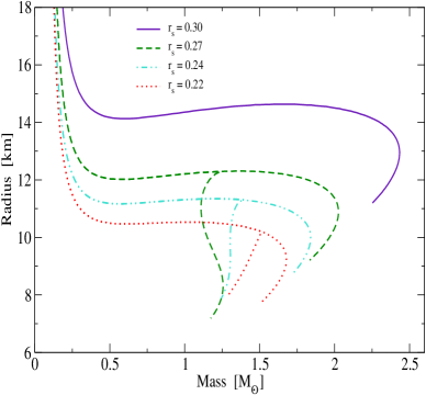
Figure 5: Mass radius relationship of neutron stars and hybrid stars for the choices of scalar attraction described in the text.

6 Discussion

We have used the NJL model, supplemented with a method of regularization which simulates confinement, to calculate consistently the properties of nuclear matter and quark matter. In doing so we have related the quark interactions in the confined phase, to the quark interactions in the deconfined phase, where color superconductivity is assumed to arise. Our principal finding is that the scalar pairing between quarks within the nucleon and in QM may be equated, if the attraction within the nucleon is attributed not only to the diquark interactions but also to the pion cloud. Since the attraction in the scalar $\overline{3}_{c}$ channel between (almost) current quarks at high densities or energies can be derived directly from QCD, this result lends some support to the Faddeev approach to the nucleon, since the quark-diquark picture may be characterized by not only the same type of pairing interaction but also the same strength as we expect to find in the high density QM phase. This is an important feature of nucleon dynamics and is relevant to any finite density studies that incorporate nucleon structure.

By including the pion cloud contributions to the nucleon mass, we found that the equation of state of nuclear matter becomes softer, reducing the neutron star and hybrid star masses significantly.

Acknowledgments S.L. would like to thank Ian Cloet for helpful discussions. This work was supported by the Australian Research Council and DOE contract DE-AC05-84ER40150, under which SURA operates Jefferson Lab, and by the Grant in Aid for Scientific Research of the Japanese Ministry of Education, Culture, Sports, Science and Technology, Project No. C2-16540267.

References

- [1] W. Bentz and A.W. Thomas, Nucl. Phys. A 696 (2001) 138.
-
[2]
P.A.M. Guichon, Phys. Lett.B 200 (1988) 235;
P.A.M. Guichon and A.W. Thomas, Phys. Rev. Lett. 93 (2004) 132502. - [3] A.H. Rezaeian and H. Pirner, arXiv:nucl-th/0510041
- [4] A.W. Thomas et. al., Prog.Theor.Phys.Suppl. 156 (2004) 124-136.
- [5] B.D. Serot and J.D. Walecka, Adv. Nucl. Phys. 11 (1986) 1.
- [6] F. Wilczek, arXiv:hep-ph/0409168
- [7] E. Santopinto, Phys. Rev. C 72 (2005) 022201(R).
- [8] S. Capstick and N. Isgur, Phys. Rev. D 34 2809 (1986).
- [9] G. Lugones and I. Bombaci, Phys. Rev. D 72 (2005) 065021; D. H. Rischke, Prog. Part. Nucl. Phys. 52 (2004) 197; T. Schäfer and F. Wilczek, Phys. Rev. D 60 (1999) 114033; H. Grigorian, D. Blaschke and D. N. Aguilera, Phys. Rev. C 69 (2004) 065802.
- [10] D. Bandyopadhyay, arXiv:nucl-th/0512100
- [11] M. Alford, arXiv:nucl-th/0512005
- [12] F. Weber, Prog. Part. Nucl. Phys. 54 (2005) 193 and references therein.
- [13] P. Wang et. al., Phys. Rev. C 72 (2005) 045801.
- [14] N. Itoh, Prog. Theor. Phys. 44 (1970) 291.
- [15] M. Buballa, Phys. Rep. 407 (2005) 205.
- [16] D. Blaschke et. al., Phys. Rev. D 72 (2005) 065020.
- [17] S. Rüster, V. Werth, M. Buballa, I.A. Shovkovy and D.H. Rischke, Phys. Rev. D 72 (2005) 034004.
- [18] M. Buballa et. al., Phys. Lett. B 595 (2004) 36-43.
- [19] L. y. He, M. Jin and P. f. Zhuang, Phys. Rev. D 71 (2005) 116001.
- [20] A. Barducci, R. Casalbuoni, G. Pettini and L. Ravagli, Phys. Rev. D 71 (2005) 016011.
- [21] D. Ebert and K.G. Klimenko, arXiv:hep-ph/0507007
- [22] T. Maruyama et. al., Nucl.Phys. A 760 (2005) 319-345.
- [23] H.J. Warringa, D. Boer and J.O. Andersen, Phys. Rev. D 72 (2005) 014015.
-
[24]
Y. Nambu and G. Jona-Lasinio, Phys. Rev. 122 (1960)
345;
124 (1961) 246;
see also, U. Vogl and W. Weise, Prog. Part. Nucl. Phys. 27 (1991) 195. - [25] M. Buballa, Nucl.Phys. A 611 (1996) 393-408.
- [26] V. Koch et. al., Phys. Lett. B 185, (1987) 1.
- [27] J. da Providencia et. al, Phys. Rev. D 36 (1987) 1882.
- [28] N. Ishii, W. Bentz and K. Yazaki, Nucl. Phys. A 578 (1995) 617.
- [29] S.P. Klevansky, Rev. Mod. Phys. 64, (1992) 649.
- [30] G. Hellstern, M. Oettel, R. Alkofer and H. Reinhardt, arXiv:hhep-ph/9805393
- [31] W. Bentz, T. Horikawa, N. Ishii and A.W. Thomas, Nucl. Phys. A 720 (2003) 95.
- [32] A. Buck, R. Alkofer and H. Reinhardt, Phys. Lett. B 286 (1992) 29.
- [33] S. Lawley, W. Bentz and A.W. Thomas, Phys. Lett. B 632 (2006) 495.
- [34] I. Cloet, W. Bentz and A.W. Thomas, Phys. Lett. B 621 (2005) 246.
- [35] A.W. Thomas and W. Weise, The Structure of the Nucleon, (Wiley-VCH, Berlin, 2001).
- [36] R.D. Young et. al., Phys. Rev. D 66, 094507 (2002).
- [37] A.W. Thomas, S. Théberge and G.A. Miller, Phys. Rev. D 24 (1981) 216.
- [38] B.C. Pearce and I.R. Afnan, Phys. Rev. C 34, (1986) 991.
- [39] M. Hecht et. al., Phys.Rev. C 65 (2002) 055204.
- [40] K. Suzuki et. al., Phys.Rev.Lett. 92 (2004) 072302.
- [41] A. Arima, K. Shimizu, W. Bentz and H. Hyuga, Adv. Nucl. Phys. 18 (1987) 1.
- [42] T. Ericson and W. Weise, Pions and Nuclei, (Clarendon Press, Oxford, 1988) 137.
- [43] H. Grigorian, D. Blaschke and D.N. Aguilera, Phys. Rev. C 69 (2004) 065802;
- [44] D.N. Aguilera, D. Blaschke and H. Grigorian, Nucl. Phys. A 757 (2005) 527.
- [45] W. Detmold, G.A. Miller and J.R. Smith, nucl-th/0509033
- [46] N.K. Glendenning, Phys. Rev. D 46, (1992) 1274.
- [47] J. Negele and D. Vautherin, Nucl. Phys. A 207, (1973) 298.
- [48] J.R. Oppenheimer and G.M. Volkoff, Phys. Rev. 55 (1939) 374.
- [49] N.K. Glendenning and C. Kettner, Astron. Astrophys. 353 (2000) L9.
- [50] E.S. Fraga, R.D. Pisarski and J. Schaffner-Bielich, Phys. Rev. D 63 (2001) 121702.
- [51] K. Schertler, C. Greiner, J. Schaffner-Bielich and M.H. Thoma, Nucl. Phys. A 677 (2000) 463-490.
- [52] J.M. Lattimer and M. Prakash, Phys. Rev. Lett. 94, (2005) 111101.
- [53] M. Takahara and K. Sato, Astrophys. J. 335 (1988) 301.