Multiplicity Dependence of Partially Coherent Pion Production
in Relativistic Heavy Ion Collisions

Abstract

We investigate two- and three-particle intensity correlation functions of pions in relativistic heavy ion collisions for different colliding energies. Based on three models of particle production, we analyze the degree to which the pion sources are chaotic in the SPS S+Pb, Pb+Pb and the RHIC Au+Au collisions. The “chaoticity”, $\lambda$, of the two-particle correlation functions is corrected for long-lived resonance decays. The effect of the partial Coulomb correction is also examined. Although the partially coherent model gives a result which is consistent with that of STAR, the chaotic fraction does not exhibit clear multiplicity dependence if we take into account both the corrected chaoticity and the weight factor of the three-pion correlation function. The result of the partially-multicoherent model indicates an increasing number of coherent sources in higher multiplicity events.

1 Introduction

Pion interferometry has been regarded as an indispensable tool in relativistic heavy ion physics. Two-particle intensity interferometry can be used to determine the sizes of the collision system. This fact is known as the Hanbury Brown-Twiss (HBT) effect. For this reason, it has been used for exploring the space-time evolution of hot, dense matter created in heavy ion collisions [1]. In particular, the most recent experiment at the Relativistic Heavy Ion Collider (RHIC) obtained an interesting result which is referred to the “HBT puzzle” [2, 3]. Hydrodynamical models have failed to reproduce the experimental results of two-particle correlation functions. Hydrodynamical models are based on the assumption of local thermal equilibrium. For the early stage of the space-time evolution, the validity of this assumption is indirectly verified by the observation of the large elliptic flow at RHIC [4]. However, equilibration in the final hadronic stage is still ambiguous. Although an exponential particle spectrum is expected for a thermal source, it does not require a system that has reached local thermal equlibrium [5].

The two-particle intensity correlation function $C_{2}(\boldsymbol{p_{1}},\boldsymbol{p_{2}})$ of identical particles provides information not only on source sizes but also on the state of the source through the chaoticity, $\lambda=C_{2}(\boldsymbol{p},\boldsymbol{p})-1$. The HBT effect does not exist if the source is coherent. The chaoticity $\lambda$ is unity for a perfectly chaotic source and 0 for a coherent source, which does not induce the HBT effect. In multi-particle production phenomena of relativistic heavy ion collisions, the thermalized source can be chaotic and non-thermal components can be coherent. For example, if disoriented chiral condensate domains are created, such domains can decay into coherent pions. Thus the final state pions may carry information regarding how partons hadronize if the deconfined phase has been created. Therefore, the chaoticity $\lambda$ is a very important quantity to investigate the final state in heavy ion collisions.

However, $\lambda$ cannot be regarded as the true chaoticity in real (experimental) situations, because many other effects, such as long-lived resonance decay contributions [6, 7, 8, 9], Coulomb repulsions, and particle contaminations [10] affect the chaoticity $\lambda$. As an alternative tool, the three-particle correlation function has been proposed [11, 12, 13, 14]. Three-particle correlations are more useful for this purpose, because long-lived resonances do not affect the normalized three-pion correlator,

$$r_{3} (\boldsymbol{p}_{1},\boldsymbol{p}_{2},\boldsymbol{p}_{3})$$

$$=\frac{[C_{3}(\boldsymbol{p}_{1},\boldsymbol{p}_{2},\boldsymbol{p}_{3})-1]-[C_{2}(\boldsymbol{p}_{1},\boldsymbol{p}_{2})-1]-[C_{2}(\boldsymbol{p}_{2},\boldsymbol{p}_{3})-1]-[C_{2}(\boldsymbol{p}_{3},\boldsymbol{p}_{1})-1]}{\sqrt{[C_{2}(\boldsymbol{p}_{1},\boldsymbol{p}_{2})-1][C_{2}(\boldsymbol{p}_{2},\boldsymbol{p}_{3})-1][C_{2}(\boldsymbol{p}_{3},\boldsymbol{p}_{1})-1]}},$$ (1)

with $C_{3}(\boldsymbol{p_{1}},\boldsymbol{p_{2}},\boldsymbol{p_{3}})$ being the three-particle correlation function [15]. The correlation functions are defined as

$$C_{2}(\boldsymbol{p_{1}},\boldsymbol{p_{2}})=\frac{W_{2}(\boldsymbol{p_{1}},\boldsymbol{p_{2}})}{W_{1}(\boldsymbol{p_{1}})W_{1}(\boldsymbol{p_{2}})}$$ (2)

and

$$C_{3}(\boldsymbol{p_{1}},\boldsymbol{p_{2}},\boldsymbol{p_{3}})=\frac{W_{3}(\boldsymbol{p_{1}},\boldsymbol{p_{2}},\boldsymbol{p_{3}})}{W_{1}(\boldsymbol{p_{1}})W_{1}(\boldsymbol{p_{2}})W_{1}(\boldsymbol{p_{3}})}$$ (3)

with $W_{n}(\boldsymbol{p_{1}},\cdots,\boldsymbol{p_{n}})$ being the $n$ particle distribution. The index of the source chaoticity in the three-pion correlator is the weight factor

$$\omega=r_{3}(\boldsymbol{p},\boldsymbol{p},\boldsymbol{p})/2$$ (4)

which is unity for a chaotic source. Due to insufficient statistics, the three-pion correlator measured in experiments to this time is slightly different from Eq. (1),

$$r_{3}(Q_{3})=\frac{[C_{3}(Q_{3})-1]-[C_{2}(Q_{12})-1]-[C_{2}(Q_{23})-1]-[C_{2}(Q_{31})-1]}{\sqrt{[C_{2}(Q_{12})-1][C_{2}(Q_{23})-1][C_{2}(Q_{31})-1]}},$$ (5)

where $Q_{ij}=\sqrt{-(p_{i}-p_{j})^{2}}$ and $Q_{3}=\sqrt{Q_{12}^{2}+Q_{23}^{2}+Q_{31}^{2}}$. The weight factor is defined as $\omega=r_{3}(0)/2$, so that it is expected to be the same as the definition Eq. (4).

As shown in a previous work [16], more precise information concerning the source can be extracted using model analyses combining two- and three-particle correlations. In this paper, we analyze the two-pion and three-pion correlations and investigate the chaoticity of the pion sources. Firstly, assuming that the main background contribution is a long-lived resonance decay and other effects are successfully removed in the experimental data, we make a correction to account for the long-lived resonance decays to the chaoticity of the two-pion correlation functions, with the help of a statistical model. Secondly, we extract the weight factor $\omega$ through the simultaneous construction of $C_{2}$ and $C_{3}$. Finally, we carry out model analyses using the “true” chaoticity $\lambda^{\text{true}}$ after applying the resonance correction and the weight factor $\omega$. In addition to the analysis of Au+Au collisions at the RHIC given in a previous paper [17], we give analyses on lower colliding energy collisions at the CERN Super Proton Synchrotron (SPS) based on the same method. We treat data from 200$A$ GeV (laboratory system) S+Pb collisions measured by the NA44 collaboration [18, 19, 20] and data from 158$A$ GeV (lab. sys) Pb+Pb collisions measured by the NA44 collaboration [21, 22] and the WA98 collaboration [23, 24]. On the basis of the results obtained from these experimental data, we investigate the multiplicity dependence of the extracted model parameters.

In the next section, we explain the three models used in this paper. The correction to account for the long-lived resonance decays is discussed §3. In §4, we will give a combined analysis of the 2$\pi$ and 3$\pi$ correlation functions, with the goal of extracting the weight factor $\omega$. The results of the model analyses are given in §5. The paper is summarized in §6.

2 Model description

We use three kinds of models in this analysis. In all the models, $\lambda^{\text{true}}$ and $\omega$ are used as inputs to fix the model parameters. The output quantities are the chaotic fraction and the mean number of coherent sources. Here we do not discuss the origin of the coherences in these models. Figure 1 presents a schematic depiction of the models.

Figure 1: Schematic depiction of Models I–III. The shaded area denote the chaotic sources. The unshaded area and the small circles represent the coherent sources. (a) Model I, (b) Model II, (c) Model III.

One is a partially coherent model [12] whose only parameter is the chaotic fraction, $\varepsilon_{\text{I}}$, defined as the ratio of the number of particles coming from the chaotic source to the total number of particles. In this model, pions are emitted from a mixture of a chaotic and a coherent source. In general, we need to fix the source function in a manner that depends on the momentum. In the present analysis, fortunately, the true chaoticity $\lambda^{\text{true}}$ and the weight factor $\omega$ are given by the correlation functions at vanishing relative momenta, and hence they can be expressed in terms of the chaotic fraction. The relations among $\varepsilon_{\text{I}}$, $\lambda^{\text{true}}$ and $\omega$ are

$$\lambda^{\text{true}}=\varepsilon_{\text{I}}(2-\varepsilon_{\text{I}}),\quad\omega=\sqrt{\varepsilon_{\text{I}}}\frac{3-2\varepsilon_{\text{I}}}{(2-\varepsilon_{\text{I}})^{3/2}}.$$ (6)

We refer to this model as Model I.

The second model, referred to as Model II, is a multicoherent source model [14]. The parameter in this model is the mean number of coherent sources, $\alpha_{\text{II}}$, which obeys the Poisson distribution. Because small coherent sources are independent, a chaotic source is realized as a cluster of an infinite number of coherent sources. The parameter $\alpha_{\text{II}}$ is thus related to $\lambda^{\text{true}}$ and $\omega$ as

$$\lambda^{\text{true}}=\frac{\alpha_{\text{II}}}{\alpha_{\text{II}}+1},\quad\omega=\frac{1}{2}\frac{2\alpha_{\text{II}}^{2}+2\alpha_{\text{II}}+3}{\alpha_{\text{II}}^{2}+3\alpha_{\text{II}}+1}\sqrt{\frac{\alpha_{\text{II}}+1}{\alpha_{\text{II}}}}.$$ (7)

As shown in Fig. 2 of Ref. Nakamura_PRC61, $\omega$ as a function of $\alpha_{\text{II}}$ has a minimum value $\omega_{\text{min}}\simeq 0.82$. Hence, there is no corresponding $\alpha_{\text{II}}$ for $\omega$ smaller than $\omega_{\text{min}}$.

As each of these models possesses only a single parameter, the parameters calculated from $\lambda^{\text{true}}$ and $\omega$ should give the same value if all corrections are correctly made.

Model III is a “partially multicoherent” source model [14]. This model is a mixture of Model I and Model II, and its parameters are the chaotic fraction $\varepsilon_{\text{III}}$ and the mean number of coherent sources $\alpha_{\text{III}}$, which are related to $\lambda^{\text{true}}$ and $\omega$ as

$$\lambda^{\text{true}} =\frac{\alpha_{\text{III}}}{\alpha_{\text{III}}+(1-\varepsilon_{\text{III}})^{2}},$$ (8)

$$\omega =\frac{2\alpha_{\text{III}}^{2}+2\alpha_{\text{III}}(1-\varepsilon_{\text{III}})^{2}+3(1-\varepsilon_{\text{III}})^{3}(1-2\varepsilon_{\text{III}})}{2[\alpha_{\text{III}}^{2}+3\alpha_{\text{III}}(1-\varepsilon_{\text{III}})^{2}+(1-\varepsilon_{\text{III}})^{3}]}\sqrt{\frac{\alpha_{\text{III}}+(1-\varepsilon_{\text{III}})^{2}}{\alpha_{\text{III}}}}.$$ (9)

In this model, there are two parameters that correspond to two experimentally measurable quantities, $\lambda^{\text{true}}$ and $\omega$. Below, we investigate the allowed parameter regions for given sets of $\lambda^{\text{true}}$ and $\omega$.

3 Extracting $\lambda^{\text{true}}$ from two-pion correlations

In relativistic heavy ion collisions, a non-negligible fraction of pions comes from the decay of long-lived resonances. Recent analyses based on statistical models show that hadrons are chemically frozen near the critical temperature $T_{c}$ [25]. Short-lived resonances, such as $\rho$ and $\Delta$, decay before hadrons reach the kinetic freeze-out or soon after the freeze-out, but long-lived resonances, such as hyperons, can decay long after the kinetic freeze-out of pions. In the two-pion correlation function, these long-lived resonances appear as a spike near $q\sim 0$, whose width is too small to be resolved with the current experimental resolutions, $\Delta q\simeq 5-10$ MeV. Thus, chaoticities $\lambda^{\text{exp}}$ measured experimentally are smaller than the true chaoticities due to long-lived resonance decays [7, 9, 26]. Following Ref. Wiedemann_PRC56, we take into account resonances up to $\Sigma^{*}(1385)$. We treat resonances whose widths are less than 5 MeV as long-lived ones, i.e., $K_{s}^{0},\eta,\eta^{\prime},\phi,\Lambda,\Sigma$ and $\Xi$ are considered long-lived resonances in the calculation. Though $\omega$ mesons have an intermediate width, it is known that they distort the shape of the correlation function at low $q$ but do not reduce the chaoticity. [7].

Table 1: Thermodynamic parameters obtained from the particle ratio in nucleus-nucleus collisions at SPS. Here, $h^{-}$ represents the negatively charged hadrons.

System	Ratio	Data [Reference]	$T$ [MeV]	$\mu_{\text{B}}$ [MeV]	$\chi^{2}/N_{\text{dof}}$
SPS S+Pb	$p/\pi^{+}$	0.18$\pm$0.03 [28, 29]	173 $\pm$ 2	196 $\pm$ 2	36/7
	$\bar{p}/p$	0.12$\pm$0.02 [30]
	$\bar{p}/\pi^{-}$	0.024$\pm$0.009 [28, 29]
	$(K^{-}+K^{+})/2K_{s}^{0}$	1.07$\pm$0.03 [31]
	$K^{+}/K^{-}$	1.67$\pm$0.15 [31]
	$K_{s}^{0}/\Lambda$	1.4$\pm$0.1 [31]
	$K_{s}^{0}/\bar{\Lambda}$	6.4$\pm$0.4 [31]
	$\bar{\Lambda}/\Lambda$	0.20$\pm$0.01 [32]
	$\Xi^{+}/\bar{\Lambda}$	0.21$\pm$0.02 [32]
SPS Pb+Pb	$\bar{p}/p$	0.085$\pm$0.009 [33]	161 $\pm$ 4	223 $\pm$ 7	44/9
	$K_{s}^{0}/\pi^{-}$	0.125$\pm$0.019 [34]
	$K_{s}^{0}/h^{-}$	0.123$\pm$0.020 [35]
	$\Lambda/h^{-}$	0.077$\pm$0.011 [35]
	$\Lambda/K_{s}^{0}$	0.63$\pm$0.08 [35]
	$\bar{\Lambda}/\Lambda$	0.131$\pm$0.017 [35]
	$\Xi^{-}/\Lambda$	0.110$\pm$0.010 [35]
	$\Xi/\bar{\Lambda}$	0.188$\pm$0.039 [36]
	$(\Xi+\bar{\Xi})/(\Lambda+\bar{\Lambda})$	0.13$\pm$0.03 [37]
	$\Xi^{+}/\Xi^{-}$	0.232$\pm$0.033 [36]
	$K^{+}/K^{-}$	1.85$\pm$0.09 [38]

For a chaotic source, the reduced chaoticity $\lambda^{\text{eff}}$ is given in terms of the ratio of the number of pions from the long-lived resonances to the total number of pions as

$$\sqrt{\lambda^{\text{eff}}}=1-\frac{N_{\pi}^{\text{r}}}{N_{\pi}},$$ (10)

where $N_{\pi}$ is the total number of emitted pions, and $N_{\pi}^{\text{r}}$ is the number of pions from the decay of long-lived resonances [9]. We calculate this ratio with the help of the statistical model. For midrapidity, the particle ratio can be written as the ratio of the number densities, i.e.,

$$\frac{N_{i}}{N_{j}}=\frac{n_{i}^{0}}{n_{j}^{0}},$$ (11)

where

$$n_{i}^{0}=\frac{g_{i}}{2\pi^{2}}\int_{0}^{\infty}dp\,p^{2}f(E,T,\mu_{\text{B}},\mu_{\text{S}},\mu_{\text{I${}_{3}$}}),$$ (12)

with $f(E,T,\mu_{j},\cdots)$ being the equilibrium distribution function and $g_{i}$ being the number of the degree of freedom of particle $i$ [27]. For simplicity, we fix the chemical potential of the third component of the isospin as $\mu_{I_{3}}=0$. Then, the thermodynamic parameters to be determined are the temperature $T$ and the baryon number chemical potential $\mu_{\text{B}}$, because the strangeness chemical potential $\mu_{S}$ is determined from the strangeness neutrality condition. Results for several collision systems obtained from the $\chi^{2}$ fit are shown in Tables 1 and 2.

Table 2: Thermodynamic parameters obtained from the particle ratio in Au+Au collisions at RHIC.

System	Ratio	Data	$T$ [MeV]	$\mu_{\text{B}}$ [MeV]	$\chi^{2}/N_{\text{dof}}$
RHIC Au+Au	$\bar{p}/p$	0.71$\pm$0.05 [39]	158 $\pm$ 9	36 $\pm$ 6	2.4/5
	$\bar{p}/{\pi^{-}}$	0.072$\pm$0.014 [40, 41]
	$K^{-}/\pi^{-}$	0.146$\pm$0.02 [42]
	$K^{*0}/h^{-}$	0.042$\pm$0.014 [43]
	$\bar{K}^{*0}/K^{*0}$	0.92$\pm$0.14 [43]
	$\bar{\Lambda}/\Lambda$	0.71$\pm$0.05 [41]
	$\bar{\Xi}/\Xi$	0.83$\pm$0.09 [43]

From Tables 1 and 2, we find that the quality of the fit becomes better as the collsion energy increases. It is reasonable to assume that the system has reached thermal equilibrium and that the pion source becomes chaotic as the collision energy increases. Below we see whether this naive assumption is valid.

Since this particle ratio is obtained from the particle numbers integrated with the particle momenta, $\lambda^{\text{eff}}$ is calculated from Eqs. (10)–(12) using the integrated particle numbers. The measured chaoticity $\lambda^{\text{exp}}$, however, depends on the average momentum of pion pairs. For example, STAR has measured $\lambda^{\text{exp}}$ for three bins of the transverse momentum ($k_{t}$) [44]. In this paper, we assume, for simplicity, that the true chaoticity $\lambda^{\text{true}}$ does not depend on the particle momentum. Therefore, we need to average $\lambda^{\text{exp}}$ over the momenta in order to evaluate $\lambda^{\text{true}}$. Assuming the $k_{t}$ dependence of the measured $\lambda^{\text{exp}}$ is dominated by long-lived resonances [i.e., Eq. (10)], we obtain the averaged chaoticity $\overline{\lambda}^{\text{exp}}$ as

$$\overline{\lambda}^{\text{exp}}=\frac{\displaystyle\sum_{i=1}^{n}\lambda^{\text{exp}}_{i}\int_{i\text{-th bin}}k_{t}dk_{t}\left(\frac{dN}{k_{t}dk_{t}}\right)^{2}}{\displaystyle\sum_{i=1}^{n}\int_{i\text{-th bin}}k_{t}dk_{t}\left(\frac{dN}{k_{t}dk_{t}}\right)^{2}},$$ (13)

with $\lambda_{i}^{\text{exp}}$ being the measured chaoticity in the $i$-th $k_{t}$ bin. [See the appendix of Ref. Morita_3pirhic for the derivation of Eq. (13).] The transverse momentum distribution $dN/k_{t}dk_{t}$, in the above equation is taken from experimental results. For S+Pb collisions, in which three-particle correlation data are available only for minimum-bias data, we calculate $\overline{\lambda}^{\text{exp}}$ by simply averaging the $\lambda^{\text{exp}}$ with different multiplicities. This should not affect our conclusion, because the data exhibit little multiplicity dependence [19]. For $\lambda^{\text{exp}}$, it is known that the value of $C_{2}(\boldsymbol{q})-1$ at $\boldsymbol{q}=0$ depends on the dimension of the projection onto $\boldsymbol{q}$-space. In general, the value of $\lambda^{\text{exp}}$ obtained from the 1-dimensional Gaussian fitting differs from that obtained from the 3-dimensional Gaussian fitting because of the projection, experimental resolution, and other effects, though these should be the same for an ideal measurement. In this paper, we use the value extracted from the 3-dimensional Gaussian fitting,

$$C_{2}^{\text{fit}}(\boldsymbol{q})=1+\lambda^{\text{exp}}\exp\left(-R_{\text{side}}^{2}q_{\text{side}}^{2}-R_{\text{out}}^{2}q_{\text{out}}^{2}-R_{\text{long}}^{2}q_{\text{long}}^{2}\right).$$ (14)

as $\lambda^{\text{exp}}$.

The true chaoticity is then given by $\lambda^{\text{true}}=\overline{\lambda}^{\text{exp}}/\lambda^{\text{eff}}$. Results for $\lambda^{\text{true}}$ obtained from various systems are summarized in Table 3. The error on $\lambda^{\text{true}}$ is the sum of the experimental one on $\overline{\lambda}^{\text{exp}}$, calculated from the errors on $\lambda_{i}^{\text{exp}}$ and $dN/k_{t}dk_{t}$, and the errors propagated from the fit of the thermodynamic quatities at the 1-$\sigma$ level, shown in Tables 1 and 2.

Table 3: Summary of $\lambda^{\text{true}}$

System	Experiment [Reference]	$\overline{\lambda}^{\text{exp}}$	$\lambda^{\text{true}}$	$\lambda^{\text{true}}_{\text{pc}}$
SPS S+Pb	NA44, min.bias [19]	0.585 $\pm$ 0.06	0.94 $\pm$ 0.06	0.7$\lambda^{\text{true}}$
SPS Pb+Pb	NA44 Central [21]	0.55 $\pm$ 0.03	0.98 $\pm$ 0.03	0.8$\lambda^{\text{true}}$
SPS Pb+Pb	WA98 Central [24]	0.58 $\pm$ 0.04	1.03 $\pm$ 0.04	0.8$\lambda^{\text{true}}$
RHIC Au+Au	STAR Central [44]	0.57 $\pm$ 0.06	0.93 $\pm$ 0.08	0.8$\lambda^{\text{true}}$

From Table 3, we see that the value of $\lambda^{\text{true}}$ are not so different and become close to unity in all systems. However, it should be noted that there may be an overestimation in $\lambda^{\text{exp}}$ due to an overcorrection for the Coulomb interaction. Because the two-pion correlation function is affected by the Coulomb interaction between the two detected pions, there are many issues concerning how the Coulomb interaction can be subtracted from the observed correlation function [45, 46, 47, 48]. Recently, it has been shown that a new procedure called the partial Coulomb correction, leads to significant correction to the source sizes [49, 10]. Such corrections are known to partially resolve the “HBT puzzle”, that $R_{\text{out}}$ becomes smaller than $R_{\text{side}}$, though this correction does not completely resolve this puzzle. In this paper, we stress that the partial Coulomb correction affects not only the source size but also the observed chaoticity, $\lambda^{\text{exp}}$. For example, CERES reports that the $k_{t}$ dependent correction to $\lambda^{\text{exp}}$ reaches 15–40 % [10]. This is a significant correction. Unfortunately, partially corrected data for the collisions that we treat in this paper (S+Pb, Pb+Pb at the SPS and Au+Au at 130$A$ GeV) are not available. Ideally, these data should be treated within a theoretical approach with a Coulomb correction [50], but this is beyond the scope of this paper. In the further analyses given in §5, we also present the results obtained using “partially corrected” $\lambda^{\text{exp}}$ in order to see how the results change when $\lambda^{\text{exp}}$ is reduced. Following the report from CERES [10], according to which the correction is larger at smaller $k_{t}$, and considering that the two-particle data used here are those of the lowest momentum bin, we simply multiplied a correction factor of 0.8 except in the S+Pb case, where the correction factor is set to 0.7, because only S+Pb data are corrected by the Gamow factor. We denote this “partially Coulomb corrected”$\lambda^{\text{true}}$ by $\lambda^{\text{true}}_{\text{pc}}$.

4 Extraction of the weight factor $\omega$

4.1 Procedure

In the previous section, we extracted $\lambda^{\text{true}}$ from the two-particle correlation data. Next, we must determine the weight factor $\omega$ in order to analyze the degree to which the pion sources are chaotic by using the models, especially Model III [Eq. (8)]. To obtain $\omega=r_{3}(0)/2$, we must extrapolate $C_{2}$ and $C_{3}$ to $\boldsymbol{q}=0$. The method of extrapolation is described in a previous paper [17] in detail. Here we briefly review the procedure.

In experimental papers, $\omega$ is extracted by simply averaging $r_{3}(Q_{3})$ (NA44 [20, 22], WA98 [24]), in which there is little dependence on $Q_{3}$, or using quadratic and quartic fits (STAR [51]). A shortcoming of these methods is that the $Q_{3}$ dependence of $r_{3}$ may be more complex than quadratic or quartic [13]. Such $Q_{3}$ dependences result from both an asymmetry of the source and coherence. In this paper, we assume observed $Q_{3}$ dependences are due to coherence. This is an assumption, but it is plausible, because the asymmetry of the source causes a $Q_{3}$ dependence of $r_{3}$ that is somewhat different from that in the observed $r_{3}$ data [13]. We reproduce $C_{2}(Q_{\text{inv}})$ and $C_{3}(Q_{3})$ using a common source function with a set of parameters which is determined by minimizing $\chi^{2}$ with respect to the experimental data. Then, we evaluate $C_{2}(0)$ and $C_{3}(0)$. The quantity $r_{3}(Q_{3})$ is also calculated for a consistency check. For simplicity, we use a spherically symmetric Fourier-transformed source function with simulateneous emission, $F_{ij}=f_{ij}(|\boldsymbol{q}_{ij}|)e^{i(E_{i}-E_{j})t_{0}}$, in which the exponential term corresponds to emission at a constant time $t_{0}$. The assumption of simulateneous emission should be a good approximation, because the experimental data suggest emissions of short duration throughout the broad range of colliding energies [44]. Since the finite emission time duration is not related to $\lambda^{\text{true}}$ but, rather, to the width of the outward correlation functions, it does not affect our results below. For the spatial part, $f_{ij}(|\boldsymbol{q}_{ij}|)$, we try the following three kinds of source functions:

$$f_{1,ij}(|\boldsymbol{q}_{ij}|) =\exp\left(-R^{2}|\boldsymbol{q}_{ij}|^{2}/2\right),$$ (15)

$$f_{2,ij}(|\boldsymbol{q}_{ij}|) =\exp\left(-R|\boldsymbol{q}_{ij}|/2\right),$$ (16)

$$f_{3,ij}(|\boldsymbol{q}_{ij}|) =\frac{1}{\sqrt{\cosh(R|\boldsymbol{q}_{ij}|)}}.$$ (17)

Here, $\boldsymbol{q}_{ij}=\boldsymbol{p}_{i}-\boldsymbol{p}_{j}$ and $R$ is a size parameter which is to be determined by the $\chi^{2}$ fitting. The third function, Eq. (17), is chosen so as to be quadratic at small $|\boldsymbol{q}|$ and exponential at large $|\boldsymbol{q}|$.

The two- and three-particle correlation functions are then calculated using the relations

$$C_{2}(\boldsymbol{p_{1},p_{2}}) =1+\lambda_{\text{inv}}\frac{f_{12}^{2}}{f_{11}f_{22}},$$ (18)

$$C_{3}(\boldsymbol{p_{1},p_{2},p_{3}}) =1+\nu\left(\sum_{(i,j)}\frac{f_{ij}^{2}}{f_{ii}f_{jj}}+2\nu_{3}\frac{f_{12}f_{23}f_{31}}{f_{11}f_{22}f_{33}}\right).$$ (19)

where $\lambda_{\text{inv}}$, $\nu$ and $\nu_{3}$ are phenomenological adjustable parameters accounting for the non-trivial coherence effect. The summation $\Sigma_{(i,j)}$ here runs over $(i,j)=(1,2),(2,3),(3,1)$. The quantities $\lambda_{\text{inv}}$, $\nu$ and $\nu_{3}$ are unity in the case of a fully chaotic source. We can set $\nu_{3}=1$ for a description of $C_{3}(Q_{3})$ at small $Q_{3}$ [17]. Then, $\lambda_{\text{inv}}$ and $\nu$ are determined by the $\chi^{2}$ fitting, like $R$. We stress that the $\chi^{2}$ fit is carried out simultaneously for the two- and three-particle correlation data.

The results of the $\chi^{2}$ fittings to the experimental data and the resultant $\omega$ are listed in Table 4.

Table 4: Results of the $\chi^{2}$ fitting to $C_{2}$ and $C_{3}$

system	$f(|\boldsymbol{q}|)$	$R$ [fm]	$\lambda_{\text{inv}}$	$\nu$	$\chi^{2}/\text{dof}$	$\omega$
SPS S+Pb	$f_{1}$	4.85$\pm$0.31	0.49$\pm$0.04	0.34$\pm$0.04	2.3/7	0.33$\pm$0.38
(NA44) [18, 20]	$f_{2}$	7.55$\pm$0.84	0.79$\pm$0.10	0.61$\pm$0.09	3.9/7	0.48$\pm$0.45
	$f_{3}$	8.99$\pm$0.80	0.55$\pm$0.06	0.40$\pm$0.05	1.9/7	0.40$\pm$0.44
SPS Pb+Pb	$f_{1}$	7.37$\pm$0.61	0.54$\pm$0.05	0.49$\pm$0.07	1.2/6	1.06$\pm$0.59
(NA44) [21, 22]	$f_{2}$	11.4$\pm$1.5	0.83$\pm$0.11	0.85$\pm$0.16	2.7/6	1.16$\pm$0.69
	$f_{3}$	13.8$\pm$1.5	0.61$\pm$0.07	0.58$\pm$0.10	0.9/6	1.15$\pm$0.67
SPS Pb+Pb	$f_{1}$	7.73$\pm$0.10	0.36$\pm$0.01	0.29$\pm$0.01	113/17	0.81$\pm$0.12
(WA98) [24]	$f_{2}$	14.2$\pm$0.29	0.75$\pm$0.02	0.62$\pm$0.02	14/17	0.68$\pm$0.12
	$f_{3}$	15.8$\pm$0.28	0.47$\pm$0.01	0.39$\pm$0.01	17/17	0.78$\pm$0.14
RHIC Au+Au	$f_{1}$	7.0$\pm$0.07	0.54$\pm$0.01	0.48$\pm$0.01	110/30	0.958$\pm$0.09
(STAR) [44, 51]	$f_{2}$	14.4$\pm$0.2	1.18$\pm$0.03	1.08$\pm$0.03	79.7/30	0.736$\pm$0.09
	$f_{3}$	15.2$\pm$0.2	0.71$\pm$0.01	0.64$\pm$0.02	15.8/30	0.872$\pm$0.097

4.2 SPS S+Pb

Figure 2: Two-pion correlation function $C_{2}(Q_{\text{inv}})$ in the (a) S+Pb collisions at the SPS, (b) Pb+Pb collisions at the SPS, measured by NA44, (c) Pb+Pb collisions at the SPS, measured by WA98, and (d) Au+Au collisions at the RHIC. The lines represent our results for the fits of each source function (see text). Filled circles represent the experimental results (SPS S+Pb by NA44[18], SPS Pb+Pb by NA44[21]and WA98[24], and RHIC Au+Au by STAR[44]).

Figure 3: Three-pion correlation function $C_{3}(Q_{3})$ in the various collisions. The identification of the symbols is the same as in Fig. 2. The experimental results presented in (a)–(d) are taken from Refs. NA44_3pi_SPb, NA44_3pi_pbpb, WA98_pbpb_prc, and STAR_3pi, respectively.

Figure 4: The normalized three-pion correlator $r_{3}(Q_{3})/2$. The identification of the symbols is the same as in Fig. 2. The experimental results presented in (a)–(d) are taken from Refs. NA44_3pi_SPb,NA44_3pi_pbpb, WA98_pbpb_prc, and STAR_3pi, respectively. The dot-dashed line in (a) represents the uncertainty propagated from the fitting parameters for the “cosh” case (see text).

Comparisons of the fitting results and the experimental data are displayed in Figs. 2(a), 3(a) and 4(a). The curves in Figs. 2(a) and 3(a) are fitted to the data using three kind of source functions: Gaussian [Eq. (15)], exponential [Eq. (16)] and cosh [Eq. (17)]. The fitting range is $0<Q_{ij},Q_{3}<60$ MeV, which is adjusted to the available $Q_{3}$ range for $r_{3}(Q_{3})$. In the case of $C_{2}$, we see that the experimental data are fit well by a quardratic function at small $Q_{\text{inv}}$ and an exponential function at large $Q_{\text{inv}}$. For this reason, the $\chi^{2}$ values in the exponential case and the Gaussian case are larger than those in the cosh case. A similar tendency is also seen in the case of $C_{3}$, though the exponential case is not excluded by the data point at the smallest $Q_{\text{inv}}$. The value of $r_{3}$ obtained from the fitted $C_{2}$ and $C_{3}$ do not differ greatly. With a simple naked-eye extrapolation in Fig. 4(a), it appears that $\omega=r_{3}(0)/2$ becomes $\sim$0.4 for all source functions. Taking the smallest $\chi^{2}$ value, we adopt the cosh case and obtain $\omega=0.40\pm 0.44$. Note that, by the definition of $r_{3}(Q_{3})$, where $C_{2}(Q_{ij})-1$ is in the denominator, there exists a large uncertainty in the calculated $r_{3}(Q_{3})$ value, because of the errors on $\lambda_{\text{inv}}$. In Fig. 4(a), we plot the error band for the cosh case. The uncertainty 0.44 associated with $\omega$ is also obtained by extrapolation of the error band to $Q_{3}=0$.

4.3 SPS Pb+Pb

For Pb+Pb collisions at 158$A$ GeV, we compared our results to data measured by both NA44 and WA98. Figures 2(b), 3(b) and 4(b) plot the results of the $\chi^{2}$ fit to the NA44 data and Figs. 2(c), 3(c) and 4(c) plot those for the WA98 data. The fitting ranges are adjusted to the available $r_{3}(Q_{3})$ data range, as in the S+Pb case, and we use the data for $Q_{ij},Q_{3}<60$ MeV.

Comparing our fit to the NA44 data, we find that all source functions seem to give nice descriptions of the data [see Figs. 2(b) and 3(b)]. The statistics are still insufficient, especially at low $Q_{3}$, in the three-particle correlation function to discriminate the best source function. The weight factor $\omega$ is larger than unity at the best fit value. This is associated with the large errorbars and consistent with the WA98 case within the errorbars. For further analysis (given below), we adopt the cosh case because it gives the best $\chi^{2}$ value. On the other hand, the WA98 data exhibit better statistics [see Figs. 2(c) and 3(c)]. This excludes the Gaussian case in the fit to $C_{2}$ and $C_{3}$. For the $\chi^{2}$ values, the exponential case has the best value, $\chi^{2}/\text{dof}=14/17$. This tendency seems to be different from that in the NA44 case. In Ref. WA98_pbpb_prc, the three-particle correlation function is fit well by a double-exponential correlation function. Although the exponential case seems to be the best of the three, $r_{3}(Q_{3})$ from the exponential source function deviates from the experimental result [Fig. 4(c)]. This should not be regarded as a serious problem, however, because errors on $\lambda_{\text{inv}}$ and $\nu$ lead to an uncertainty on $r_{3}(Q_{3})$, as shown in the SPS S+Pb case [Fig. 4(c)]. A likely reason for this deviation is that $C_{3}(Q_{3})$ is smaller than that obtained from the experimental data in the exponential case at low $Q_{3}$. Naive extrapolation by naked eye in Fig. 4(c) again suggests that the cosh or Gaussian case is better, but this may be a coincidence in the Gaussian case, because both $C_{2}$ and $C_{3}$ deviate from the experimental data at low relative momenta. Hence, we adopt the cosh case as the result for $\omega$. Despite the different behavior of $C_{3}(Q_{3})$, the result for $\omega$ obtained from the WA98 data is consistent with the that obtained from the NA44 data.

4.4 RHIC Au+Au

Results presented in this subsection are the same as those presented in Ref. Morita_3pirhic. Figures 2(d), 3(d) and 4(d) display the correlation functions and the three-pion correlator for the Au+Au collisions at the RHIC energy. The fitting range is $0<Q_{\text{inv}}<90$ MeV for $C_{2}$ and $0<Q_{3}<100$ MeV for $C_{3}$. The high statistics of the data allows us to discriminate the source function. In the cosh case, the value of $\chi^{2}$ is much smaller than other two cases. Finally, we obtain $\omega=0.872\pm 0.097$.

5 Results and discussions

In §3, we extracted $\lambda^{\text{true}}$ from the experimental data, $\lambda^{\text{exp}}$, with the help of a statistical model. In §4, we extracted the weight factor $\omega$ from the experimental data. Now we have two input parameters for the analysis employing Models I–III. [see Eqs. (6)–(9)]. In Models I and II, there is one model parameter ($\varepsilon_{\text{I}}$ for Model I and $\alpha_{\text{II}}$ for Model II) corresponding to the two input quantities, $\lambda^{\text{true}}$ and $\omega$. We determined the model parameters by minimizing

$$\chi^{2}\equiv\frac{[\lambda^{\text{true}}_{\text{exp}}-\lambda^{\text{true}}_{\text{cal}}]^{2}}{(\delta\lambda^{\text{true}}_{\text{exp}})^{2}}+\frac{[\omega_{\text{exp}}-\omega_{\text{cal}}]^{2}}{(\delta\omega_{\text{exp}})^{2}},$$ (20)

where $\lambda^{\text{true}}_{\text{exp}}$ and $\omega_{\text{exp}}$ were extracted from the experimental data in §3 and 4. The quantities $\delta\lambda^{\text{true}}_{\text{exp}}$ and $\delta\omega_{\text{exp}}$ are the errors on $\lambda^{\text{true}}_{\text{exp}}$ and $\omega_{\text{exp}}$, which are given in Tables 3 and 4, respectively. In Models I and II, $\lambda^{\text{true}}_{\text{cal}}$ and $\omega_{\text{cal}}$ are functions of $\varepsilon_{\text{I}}$ and $\alpha_{\text{II}}$, respectively, calculated using Eqs. (6) and (7). In Model III, we solve Eqs. (8) and (9) for the given sets of $\lambda^{\text{true}}_{\text{exp}}$ and $\omega_{\text{exp}}$ to obtain $\varepsilon_{\text{III}}$ and $\alpha_{\text{III}}$. However, solutions of these equation may exist in unphysical parameter regions, such as $\varepsilon_{\text{III}}<0$. In such cases, we determine a “Best fit” solution by minimizing the above $\chi^{2}$ within the physical model parameter region, $0\leq\varepsilon_{\text{III}}\leq 1$ and $0\leq\alpha_{\text{III}}<\infty$.

5.1 Partially coherent model (Model I)

We plot $\varepsilon_{\text{I}}$ determined from Eq. (20) as a function of the multiplicities of various collision systems in Fig. 5. We consider three cases: The open squares represent the results obtained from Eq. (20) using $(\lambda^{\text{true}},\omega)$, the solid triangles represent those obtained using $(\lambda^{\text{true}}_{\text{pc}},\omega)$, and the closed circles represent those calculated from $\omega$ only, using the second equation in Eq. (6).

While the result denoted “$\omega$ only” exhibits clear increase of $\varepsilon_{\text{I}}$ with multiplicity, which is consistent with the result obtained by the STAR[51], neither $(\lambda^{\text{true}},\omega)$ nor $(\lambda^{\text{true}}_{\text{pc}},\omega)$ exhibit such a clear dependence. This is because $\lambda^{\text{true}}$ in Table 3 does not display a clear multiplicity dependence and $\delta\lambda_{\text{exp}}^{\text{true}}\ll\delta\omega_{\text{exp}}$. The value of $\varepsilon_{\text{I}}$ which minimizes $\chi^{2}$ is mostly determined by $\lambda^{\text{true}}$ and $\lambda^{\text{true}}_{\text{pc}}$ only, i.e., the values of $\omega$ are not clearly reflected in the minimization of $\chi^{2}$ due to the fact that they possess larger errors than $\lambda^{\text{true}}$. If this model is good enough, and if the experimental background for the correlation, such as the Coulomb correction is successfully removed, the result of $(\lambda^{\text{true}}_{\text{pc}},\omega)$ should agree well with the “$\omega$ only” result. In Fig. 5, these results seem to be quantitatively consistent. If the experimental accuracy of the three-particle correlation measures improves, these results will be more conclusive.

Figure 5: $\varepsilon_{\text{I}}$ as a function of the multiplicity. For the Pb+Pb collisions at the SPS, we plot both the NA44 and WA98 data with a slightly shifted horizontal axis for a clear comparison of the results.

5.2 Multicoherent model (Model II)

Table 5: The parameter $\alpha_{\text{II}}$ in the multicoherent model (Model II)

System	From ($\lambda^{\text{true}},\omega$)	From ($\lambda^{\text{true}}_{\text{pc}},\omega$)	From $\omega$ only
SPS S+Pb	12.97${}^{+57.85}_{-6.16}$	1.93${}^{+0.41}_{-0.31}$	—
SPS Pb+Pb (NA44)	40.12${}^{+\infty}_{-23.84}$	3.55${}^{+0.67}_{-0.51}$	0.72${}^{+0.81}_{-0.38}$
SPS Pb+Pb (WA98)	201.93${}^{+\infty}_{-179.2}$	4.59${}^{+1.34}_{-0.92}$	—
RHIC Au+Au	10.54${}^{+21.03}_{-4.88}$	2.86${}^{+1.25}_{-0.76}$	7.59${}^{+9.66}_{-6.53}$

The results for $\alpha_{\text{II}}$ in the multicoherent model [Eq. (7)] are displayed in Table 5. As in the case of Model I, three cases are shown. The results for $(\lambda^{\text{true}},\omega)$ and $(\lambda^{\text{true}}_{\text{pc}},\omega)$ cases mainly reflect their $\lambda^{\text{true}}$ and $\lambda^{\text{true}}_{\text{pc}}$ values due to the fact that $\delta\lambda^{\text{true}}$ is much smaller than $\delta\omega$. In the $(\lambda^{\text{true}},\omega)$ case, $\alpha_{\text{II}}$ takes a very large value, coming from $\lambda^{\text{true}}\simeq 1$. The value of $\alpha_{\text{II}}$ in the $(\lambda^{\text{true}}_{\text{pc}},\omega)$ case is significantly smaller, but there is no clear multiplicity dependence in this case as expected from the fact that $\lambda^{\text{true}}_{\text{pc}}$ does not possess a clear multiplicity dependence. In the “$\omega$ only” case, there are no solutions for the SPS S+Pb and Pb+Pb (WA98) data (the blank entries in Table 5), because this model has no corresponding value of $\alpha_{\text{II}}$ below $\omega\simeq 0.82$ [see Fig. 2 of Ref. Nakamura_PRC61]. This implies that this model is not suitable for studying multiplicity dependence; i.e., models with a chaotic background give a better description of the data.

5.3 Partially multicoherent model (Model III)

In the analysis using Model III, there are two output parameters ($\varepsilon_{\text{III}}$ and $\alpha_{\text{III}}$) corresponding to the two inputs, $\lambda^{\text{true}}$ and $\omega$. In the following, we display the allowed regions of $\varepsilon_{\text{III}}$ and $\alpha_{\text{III}}$ which correspond to the sets of $\lambda^{\text{true}}$ and $\omega$ in Fig. 6 and $\lambda^{\text{true}}_{\text{pc}}$ and $\omega$ in Fig. 7.

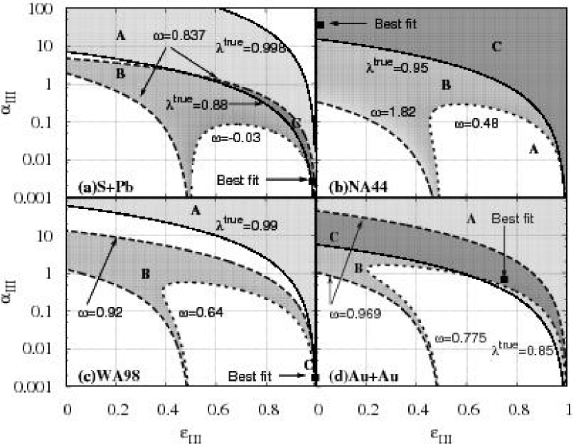
Figure 6: Allowed regions for $\lambda^{\text{true}}$ in the various systems. (See text for details.)

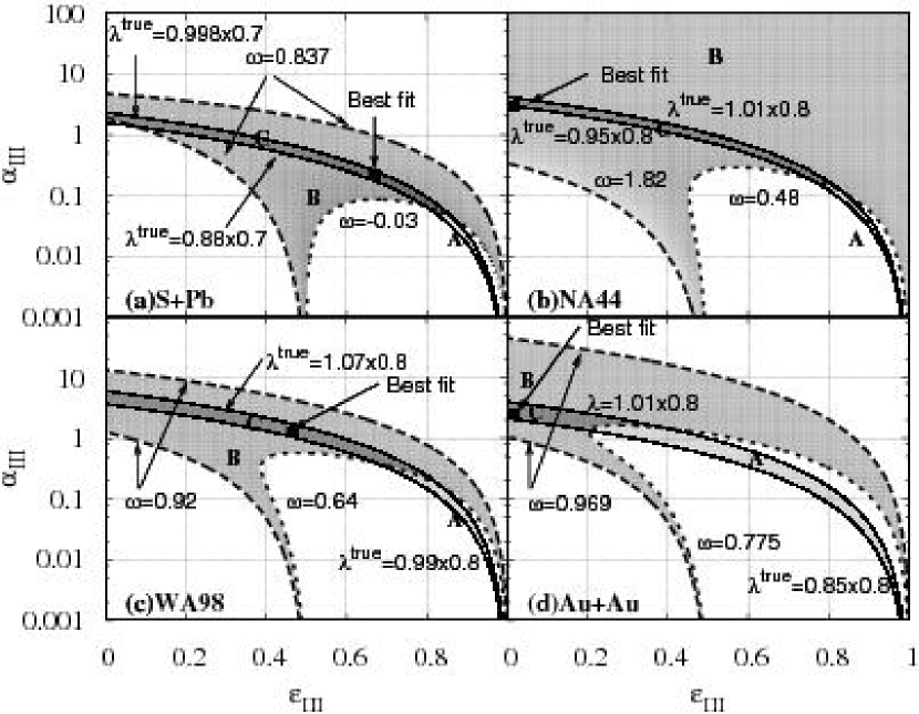
Figure 7: Allowed region for $\lambda^{\text{true}}_{\text{pc}}$ in the various systems. (See text for details.)

In each figure, the lightly shaded area labeled “A” is the allowed parameter region corresponding to the value of $\lambda^{\text{true}}$ or $\lambda^{\text{true}}_{\text{pc}}$, whose boundary is indicated by the solid line. Area B, bounded by the dashed (upper limit of $\omega$) and dotted (lower limit of $\omega$) curves, is the allowed parameter region corresponding to $\omega$. The darkest area, which is the region in which Areas A and B overlap, is Area C, which is the allowed parameter region for $\alpha_{\text{III}}$ and $\varepsilon_{\text{III}}$. The best fit values calculated from the values in Tables 3 and 4 are indicated by the squares.

Figure 6(a) plots the result for the S+Pb collisions using $\lambda^{\text{true}}$. It is seen that Area C is narrow, and the chaotic fraction has a lower bound near $\varepsilon_{\text{III}}=0.6$. The best fit value is $\varepsilon_{\text{III}}\simeq 1$ which reflects that $\lambda^{\text{true}}$ is near unity and a lower value of $\omega$. If we adopt a partially Coulomb corrected $\lambda^{\text{true}}_{\text{pc}}$, the situation changes. Due to the smaller $\lambda^{\text{true}}_{\text{pc}}$[Fig. 7(a)], $\varepsilon_{\text{III}}$ is allowed for a wider region and it has a maximum. The best fit value also shifts to $\varepsilon_{\text{III}}=0.67$ and $\alpha_{\text{III}}=0.21$. Note that, as we can see from Fig. 7, the upper bound of $\varepsilon_{\text{III}}$ is mainly dominated by the lower bound of $\omega$.

Figure 6(b) displays the allowed region from $\lambda^{\text{true}}$ and $\omega$ for the NA44 Pb+Pb collision dataset. Because the lower bound of $\lambda^{\text{true}}$ has a large value, 0.95, Area C allows both a mostly chaotic source with a small number of coherent sources and a number of the coherent sources with a small chaotic background. In this case, a solution of Eqs. (8)–(9) exists in the unphysical region, $\varepsilon_{\text{III}}=1.01$ and $\alpha_{\text{III}}=0.003$. Hence, we determine the “Best fit” point by minimizing $\chi^{2}$ in Eq. (20). The result of the minimization gives the “Best fit” at $\varepsilon_{\text{III}}=0$ and $\alpha_{\text{III}}=40.1$. This result does not always imply that the multicoherent picture is good; the difference between the value of $\chi^{2}$ for this minimum and in another case, for example, $\epsilon_{\text{III}}=0.99$ and $\alpha=0.01$, is much smaller than unity.

If we adopt the partially Coulomb corrected chaoticity $\lambda^{\text{true}}_{\text{pc}}$, Area C in Fig. 7(b) becomes narrow, as in the S+Pb case. Because the lower bound of $\omega$ is larger than that in the S+Pb case, the upper limit of $\varepsilon_{\text{III}}$ becomes smaller. Similarly, this case does not have a solution of $\varepsilon_{\text{III}}$ and $\alpha_{\text{III}}$ within the physical region ($\varepsilon_{\text{III}}=1.56$, $\alpha_{\text{III}}=1.12$), and therefore the “Best fit” point is determined by minimizing $\chi^{2}$ in Eq. (20). Though the location of the “Best fit” point corresponds to the multicoherent picture ($\varepsilon_{\text{III}}=0$), the opposite case ($\varepsilon_{\text{III}}\sim 1$) is statistically allowed for the same reason as in the previous case.

Similarly, Figs. 6(c) and 7(c) display the results for the WA98 dataset. Since the central value of $\lambda^{\text{true}}$ exceeds unity, only a very small region near $\varepsilon_{\text{III}}=1$ is allowed in Fig. 6(c). This situation changes drastically if one adopts the $\lambda^{\text{true}}_{\text{pc}}$. In Fig. 7(c), the allowed region has a shape similar to that in the NA44 case [Fig. 7(b)]. The best fit value is located at $\varepsilon_{\text{III}}=0.47$ and $\alpha_{\text{III}}=1.29$.

Finally, we display the results for Au+Au collisions at RHIC in Figs. 6(d) and 7(d). From $\lambda^{\text{true}}$ and $\omega$, it is difficult to distinguish the structure of the source; both a large chaotic fraction with a small number of coherent sources ($\varepsilon_{\text{III}}\sim 1$ and $\alpha_{\text{III}}<1$) and small chaotic fraction with a large number of coherent sources ($\varepsilon_{\text{III}}\sim 0$ and $\alpha_{\text{III}}>1$) can reproduce the experimental data. The best fit value is located at $\varepsilon_{\text{III}}=0.75$ and $\alpha_{\text{III}}=0.77$. However, if we use the partially Coulomb corrected two-particle correlation data, the allowed region is strongly restricted. Although the solution of Eqs. (8)–(9) exists in the unphysical region, $\varepsilon_{\text{III}}=-0.54$ and $\alpha_{\text{III}}=6.83$, the “Best fit” point is located at $\epsilon_{\text{III}}=0$ and $\alpha_{\text{III}}=2.86$. The maximum value allowed for $\varepsilon_{\text{III}}$ is 0.4. This means that the strong chaotic behavior observed at the RHIC is due to the production of a cluster of coherent sources.

Figure 8: The minimum (solid squares) and maximum (solid circles) value of $\alpha_{\text{III}}$ in Model III for various collisions as a function of the multiplicity. For the Pb+Pb collisions at the SPS, we plot both the NA44 and WA98 data with a slightly shifted horizontal axis for a clear comparison of the results.

As shown in the Fig. 7, the maximum bounds on $\varepsilon_{\text{III}}$ are mainly determined by the lower bounds on $\omega$, which become larger as the energy and the multiplicity increase. The fact that $\alpha_{\text{III}}$ becomes larger as the multiplicity increases is consistent with the result of a previous analysis by one of the authors (H. N.), in which the chaoticity and the weight factor were experimentally determined.[16] In Fig. 8, we plot the maximum and minimum values of $\alpha_{\text{III}}$ for the sets of $\lambda^{\text{true}}_{\text{pc}}$ and $\omega$ extracted from Fig. 7. We can see that minimum value of $\alpha_{\text{III}}$ increases with the multiplicity. This suggests that, as the collision energy and the multiplicity increase, the number of coherent sources increases. Note that the maximum values are the same as those obtained using Model II for $\lambda^{\text{true}}_{\text{pc}}$ (see Table 5), because $\alpha_{\text{III}}$ takes its maximum value when $\varepsilon_{\text{III}}=0$. Furthermore, this tendency seems to be correlated with the plausibility of the statistical model ($\chi^{2}/N_{\text{dof}}$), given in Tables 1 and 2. Though we do not know any explicit relation between Models I–III and the hadronization mechanism, this result may reflect a possible hadronization mechanism from the quark-gluon plasma phase created in the collisions.

6 Summary

In summary, we have investigated the degree to which the pion sources are chaotic in various heavy ion collisions by analyzing the two- and three-particle correlation data with three kinds of particle production models. For the two-particle correlation data, we have extracted the “true” chaoticity by considering long-lived resonance contributions to the pion multiplicity, with the help of a statistical model. Using simple source functions, we simultaneously investigated the two- and three-particle correlation functions to extract the weight factor $\omega$ of the three-particle correlator. Incorporating the chaoticity and the weight factor into the models, we have studied the chaotic fraction and mean number of the coherent sources. The results for $\varepsilon_{\text{I}}$ obtained from $\omega$ indicates that the system becomes chaotic as the multiplicity increases. This result is consistent with Ref. STAR_3pi. From a multicoherent source point of view, it is concluded that pions at higher collision energies may be emitted from a cluster of coherent sources and the number of sources increases as the collision energy and the multiplicity increase (Fig. 8).

References

- [1] B. Tomášik and U. A. Wiedemann, in Quark-Gluon Plasma 3, ed. R. Hwa and X. N. Wang (World Scientific, 2003), p. 715; hep-ph/0210250.
- [2] U. Heinz and P. Kolb, \NPA702,2002,269.
- [3] K. Morita and S. Muroya, \PTP111,2004,93, and references therein.
- [4] P. F. Kolb, P. Huovinen, U. Heinz and H. Heiselberg, \PLB500,2001,232.
- [5] D. H. Rischke, \NPA698,2002,153c.
- [6] M. Gyulassy and S. S. Padula, \PLB217,1988,181.
- [7] J. Bolz, U. Ornik, M. Plümer, B. R. Schlei and R. M.Weiner, \PRD47,1993,3860.
- [8] H. Heiselberg, \PLB379,1996,27.
- [9] T. Csörgő, B. Lörstad and J. Zimányi, Z. Phys. C71 (1996) 491.
- [10] D. Adamová et al. (CERES Collaboration), \NPA714,2003,124.
- [11] M. Biyajima, A. Bartl, T. Mizoguchi, N. Suzuki and O. Terazawa, \PTP84,1990,931.
- [12] U. Heinz and Q. H. Zhang, \PRC56,1997,426.
- [13] H. Nakamura and R. Seki, \PRC60,1999,064904.
- [14] H. Nakamura and R. Seki, \PRC61,2000,054905.
- [15] T. J. Humanic, \PRC60,1999,014901.
- [16] H. Nakamura and R. Seki, \PRC66,2002,027901.
- [17] K. Morita, S. Muroya and H. Nakamura, \PTP114,2005,583.
- [18] H. Bøggild et al. (NA44 Collaboration), \PLB302,1993,510.
- [19] K. Kaimi et al. (NA44 Collaboration), Z. Phys. C 75 (1997), 619.
- [20] H. Bøgglid et al. (NA44 Collaboration), \PLB455,1999,77.
- [21] I. G. Bearden et al. (NA44 Collaboration), \PRC58,1998,1656.
- [22] I. G. Bearden et al. (NA44 Collaboration), \PLB517,2001,25.
- [23] M. M. Aggarwal et al. (WA98 Collaboration), \PRL85,2000,2895.
- [24] M. M. Aggarwal et al. (WA98 Collaboration), \PRC67,2003,014906.
- [25] P. Braun-Munzinger, D. Magestro, K. Redlich and J. Stachel, \PLB518,2001,41.
- [26] U. A. Wiedemann and U. Heinz, \PRC56,1997,3265.
- [27] J. Cleymans and K. Redlich, \PRC60,1999,054908.
- [28] M. Murray (NA44 Collaboration), \NPA566,1994,515c.
- [29] M. Gaździcki (NA35 Collaboration), \NPA590,1995,197c.
- [30] B. Jacak (NA44 Collaboration), in Hot and Dense Nuclear Matter, ed. W. Greiner, H. Stöcker and A. Gallmann (Plenum, New York, 1994), p. 607.
- [31] D. D. Bari (WA85 Collaboration), \NPA590,1995,307c.
- [32] S. Abatzis et al. (WA85 Collaboration), \NPA566,1994,225c.
- [33] P. G. Jones (NA49 Collaboration), \NPA610,1996,188c.
- [34] D. Röhrich (NA49 Collaboration), in Proceedings of International Workshop XXV on Gross Properties of Nuclei and Nuclear Excitations, Hirschegg 1997 (1997), p. 299.
- [35] E. Andersen et al. (WA97 Collaboration), \PLB449,1999,401.
- [36] F. Gabler et al. (NA49 Collaboration), J. of Phys. G25 (1999), 199.
- [37] S. Margetis et al. (NA49 Collaboration), J. of Phys. G25 (1999), 189.
- [38] M. Kaneta et al. (NA44 Collaboration), \NPA638,1998,419c.
- [39] C. Adler et al. (STAR Collaboration), \PRL86,2001,4778. [Errata; \andvol90,2003,119903].
- [40] C. Adler et al. (STAR Collaboration), \PRL87,2001,262302.
- [41] J. Adams et al. (STAR Collaboration), \PRL567,2003,167.
- [42] C. Adler et al. (STAR Collaboration), \PLB595,2004,143.
- [43] C. Adler et al. (STAR Collaboration), \PRC66,2002,061901(R).
- [44] C. Adler et al. (STAR Collaboration), \PRL87,2001,112301.
- [45] S. Pratt, \PRC33,1986,1314.
- [46] M. G. Bowler, \PLB270,1991,69.
- [47] M. Biyajima, T. Mizoguchi, T. Osada and G. Wilk, \PLB353,1995,340.
- [48] Y. M. Sinyukov, R. Lednicky, S. V. Akkelin, J. Pluta and B. Erazmus, \PLB432,1998,248.
- [49] S. S. Adler et al. (PHENIX Collaboration), \PRL93,2004,152302.
- [50] M. Biyajima, M. Kaneyama and T. Mizoguchi, \PLB601,2004,41.
- [51] J. Adams et al. (STAR Collaboration), \PRL91,2003,262301.
- [52] U. Heinz and A. Sugarbaker, \PRC70,2004,054908.